Development and testing of geo-processing models for the automatic generation of remediation plan and navigation data to use in industrial disaster remediation

(1)

O R I G I N A L A R T I C L E

Open Access

Development and testing of geo-processing

models for the automatic generation of

remediation plan and navigation data to

use in industrial disaster remediation

G. Lucas

1,2*

, Cs. Lénárt

1

and J. Solymosi

2

Abstract

Background:This paper introduces research done on the automatic preparation of remediation plans and

navigation data for the precise guidance of heavy machinery in clean-up work after an industrial disaster. The input test data consists of a pollution extent shapefile derived from the processing of hyperspectral aerial survey data from the Kolontár red mud disaster.

Methods:Five algorithms were developed, the respective scripts were written in Python, and then tested. The first model aims at drawing a parcel clean-up plan. It tests four different parcel orientations (0, 90, 45 and 135°) and keeps the plan where clean-up parcels are less numerous. The second model uses the orientation of each contamination polygon feature to orientate the features of the clean-up plan accordingly. The third model tested if it is worth rotating the parcel features by 90° for some contamination feature. The fourth model drifts the clean-up parcel of a work plan following a grid pattern; here also with the belief to reduce the final number of parcel features. The last model aims at drawing a navigation line in the middle of each clean-up parcel.

Results:The best optimization results were achieved with the second model; the drift and 90° rotation models do not offer significant advantage. By comparison of the results between different orientations we demonstrated that the number of clean-up parcels generated varies in a range of 4 to 38 % from plan to plan.

Conclusions:Such a significant variation with the resulting feature numbers shows that the optimal orientation identification can result in saving work, time and money in remediation.

Keywords:Remediation, Clean-up, Industrial disaster, Automatic planning, Geo-processing models, GIS, Guidance, Navigation, Python, ArcPy

Background

On October 4th, 2010 Hungary faced the worst environ-mental disaster in its history when the embankment of a toxic waste reservoir failed and released a mixture of

600,000 to 700,000 m3 [1, 2] of red mud and water.

Lower parts of the settlements of Kolontár, Devecser, and Somlóvásárhely were flooded. Ten people died and another 120 people were injured [2]. The red mud flooded 4 km2of the surrounding area [3].

The idea motivating this research work came after considering the clean-up work done on the impacted area of Kolontár (to the north of Balaton). Whereas digital maps figuring the contour of the contaminated areas and the pollution thickness were available1[4], the excavation work was performed in a traditional way, without the support of positioning and navigation tech-nologies. So accurate and detailed information produced in the early stage of the remediation process was not ef-ficiently exploited.

In a broader context, our research work aims at devel-oping methodologies and tools to assure a continuum with the geographic information exploitation/support * Correspondence:[email protected]

1_{Research Institute of Remote Sensing and Rural Development, Károly Róbert} College, Gyöngyös, Hungary

2_{Doctoral School of Military Engineering, National University of Public} Service, Budapest, Hungary

(2)

through a precise remediation process. The GI gathered during the disaster assessment phase should be adapted and used in the planning phase; this would provide plans and navigation data for the clean-up phase. Additionally technologies integration (remote sensing (detection), GIS (planning), positioning and navigation (clean-up)) should also be researched.

Our bibliographic research demonstrated that the use of geoinformation technologies in remediation is mainly done during the initial stage of remediation for the detection and mapping of the pollution [5]. Aerial survey [4] and soil sampling are used for data acquisition. GIS, geo-statistical analysis and 3D modelling [6–12]; are then employed for visualizing the pollution extents, esti-mating the volume to process (project dimensioning and costs) and planning/monitoring the remediation work at the general organisational site level. In contrast, the ex-amples of use of geographic information technologies during the clean-up stage are quite few. In the case of in-situ remediation, injection and recovery wells can be precisely positioned with GPS based on planning opti-mized with geo statistic calculations [13]. In the case of

ex-situ2 remediation, literature does not mention the

use of navigation and positioning technologies for the excavation work done by heavy machineries. As posi-tioning technologies are routinely employed in civil en-gineering and agriculture [14, 15–18] for the guidance of heavy equipment for precise and efficient work it seems the shortcomings in the case of ex-situ remediation lays in the capacity to generate adequate remediation plans and in the lack of adapted GIS tools, models, methods and practice [19]. In response, this work develops models in order to be able to produce a plan containing “clean-up parcels”and derived navigation data.

“Clean-up parcel” is a central concept and the geo-graphic feature of interest in this work. Clean-up parcel in the real world corresponds with the surface covered by a dozer shovel until it gets filled to capacity (in other words the dozer’s maximum work footprint). In the GIS model a clean-up parcel consist of a rectangular feature in a polygon feature class. Its width is equal with the

dozer’s blade width. Its length (length Max) is derived

from the bulldozer characteristics and the thickness of pollution to collect (1).

Volume bladeMax¼ widthdozer lengthMax

thickness ð1Þ

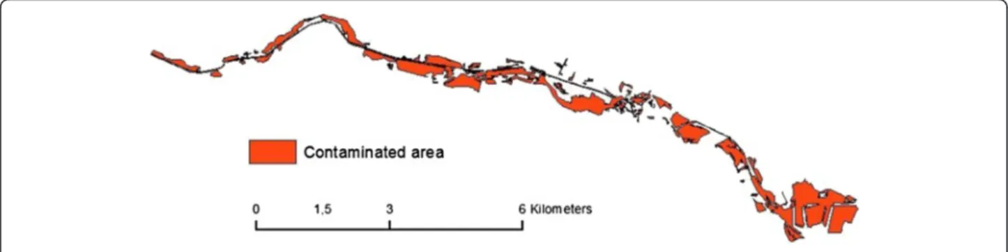
The area of interest (contaminated area) is presented in Fig. 1. It is a polygon shapefile which was created from classified hyperspectral imagery [4]. The area covers 4 km2, is 16 km long in longitude and 5 km long in latitude. Because the catastrophe was a flood, the poly-gon features of the contaminated area have an orientation that generally follows the direction of the flood.

This paper focuses exclusively on precisely describing the conception of the algorithms, architecture and how geo-processing is done rather than providing line per line calculation details and scripts. The latter can be downloaded using the following link: https://zenodo.org/ record/48883.

Readers should notice that this exploratory work is relevant for ex-situ remediation (remediation where excavation is done) on extended areas where industrial disaster took place (red mud, nuclear, chemical, etc.). In such cases heavy machinery is used and it makes sense to try to plan their moves precisely in order to save effort, time and money, in a similar way as precision agriculture or civil engineering do.

The research firstly develops models through the design of algorithms and their transcription in Python scripts. Secondly the models are tested with a test data-set derived from the red mud disaster impact assess-ment. The first test control if geo-processing is done without errors. The second test control if the model shows efficiency in its tasks consisting of optimizing the clean-up parcel plan (i.e. reducing the number of par-cels). Last, the efficiency of the model is assessed in regard to time efficiency. Based on the results of the tests diverse improvements are made, models are tested again and final versions of models are proposed.

(3)

Methods

Clean-up parcels model development (with four orientations)

Description of the objectives

This model generates a polygon feature class, containing rectangular features with a unique shape that represents the clean-up parcels. The parcel’s width is inherited from the bulldozer’s blade width. The parcel’s length is derived from the blade capacity. Dividing the contaminated area into clean-up parcels should be done automatically. The parcels should properly cover the whole contaminated area. The pattern designed should be optimal, meaning that technically it ensures the proper removal of pollution and economically it ensures the highest efficiency.

Considering those requirements it appears that rect-angular grid pattern model is optimal.

Algorithm’s raw architecture

The feature class will be similar to a grid with rectangular polygons. The algorithm could be divided into two parts:

the first part makes the calculations in order to point out to locations organised in a grid pattern with the appropriate orientation.

the second part calculates the parcel corners’ coordinates and draws rectangular polygons.

Iterations (done with loops implementing repeat/while commands) will succeed ranges calculations deriving

from the geographic extent of “Contaminated_area”.

This calculation can be separated in a function.

As the process will be automatized, it could be useful to test different plans with different orientations of the par-cels. An algorithm with four different orientations (0°, 90°, 45° and 135°) was drafted. The best result was selected by counting the number of features in each feature class cre-ated and selecting the one with the fewest parcels.

Data requirement (input)

A polygon feature class where features’geometry represents the polluted areas.

Width (in meter), length (in meter), orientation (in degree).

Algorithm architecture

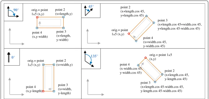
Procedure createRectangleAtPoint(x, y, length, width, orientation, layer) This procedure draws one rectangle according to the coordinates of a corner starting point, the orientation, the width and length of the rectangle. The vertices of the rectangle are attributed in the clockwise direction (Fig. 2).

Function extent(fc) This function extracts the geo-graphical extent (xmax, xmin, ymax, ymin) from a refer-ence layer; i.e. the contaminated area layer. It is used later in the calculation of the maximal limit for the iter-ation in the loops building the grids. This function already existed and we have simply re-used it [20].

Procedure Make_Grid(length, width, layer_name, grid_orientation) This procedure primarily draws a grid

45°

135° 90° orig.= point

1&5 (x,y)

point 2 (x+length,y)

point 3 (x+length, y-width) point 4

(x,y-width)

0°

orig.= point 1&5 (x,y)

point 2 (x+width,y)

point 3 (x+width, y-length) point 4

(x,y-length)

point 2 (x+length.cos 45, y+length.cos 45)

point 3

(x+length.cos 45+width.cos 45, y+length.cos 45-width.cos 45)

point 4 (x+width.cos 45, y-width.cos 45)

orig.= point 1&5

(x,y)

point 2 (x+length.cos 45, y-length.cos 45) point 3

(x+length.cos 45-width.cos 45, y-length.cos 45-width.cos 45) point 4

(x-width.cos 45, y-width.cos 45)

Fig. 2Details of the coordinate calculations with vertices of the parcel and drawing method in createRectangleAtPoint procedure with the 4

(4)

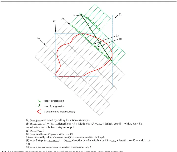
pattern taking into consideration the orientation, the width and length provided as parameters. For each point of the grid the procedure calls the createRectangleAt-Point procedure which draws a rectangle. With the 0° and 90° orientations the procedure loops top-down with the lines and left-right inside line. With the 135° and 45° orientations the procedure follows two stages which are presented in Figs. 3 and 4. In the stage 1, loop 1 creates features in diagonal starting from the top left corner (a) moving towards the bottom right corner with an incre-menttaion defined by (d). Loop 1 end when x coordinate of the pointer reach the xmax value (e). Loop 2 controls

jumping one line down under the start of previous line using incrementation (f) on back-up coordinates of previ-ous line start (b). Loop 2 ends when pointer reach ymin

value (g).

Then in a second stage, the model progress diagonally down with loop 1 and incrementation (d) but the second loop’s implementation positions the next line on top of the previous one (incrementation (f)) so that the grid can cover the second half of the area (above the stage one). As many features are created out of the area of interest, a clean-up is necessary at the end. Selection is done on the features that intersect the “polluted_area” layer. They are copied in a new layer and all temporary layers are deleted

at the end. Loop 2 ends when pointer reaches coordinate values both bigger than xmaxand ymaxvalue (g).

Script body

The algorithm uses the Procedure_Make_Grid and Pro-cedure_CreateRectangleAtPoint in order to create four feature classes with 0°, 90°, 45° and 135° orientations. Finally a“get count”method is used to retrieve the num-ber of features from each feature class. The feature class containing the smallest number of features is selected and saved; the other feature classes are deleted from the map document.

Clean up parcel model refinement (with individual and exact orientation)

Description of the objectives

In variation with the previous version (described in part 2.) the model is not intended to process groups of fea-tures from “contaminated area” but to process feature individually. The model should be designed to calculate

the orientation of each feature from “Contaminated

area”. Knowing the orientation of each feature from

“contaminated area”, it prepares a clean-up plan with the same orientation.

(a) (xmin,ymax) extracted by calling Function extend(fc)

(b) (xbackup,ybackup) = (xmin,ymax): coordinates stored before entry in loop 1

(c) (xloop1,yloop1)

(d) loop 1 step: (xloop1,yloop1) = (xloop1+width . cos 45,yloop1 - width . cos 45)

(e) xmaxextracted by calling Function extend(fc), termination condition for loop 1.

(f) loop 2 step: (xbackup,ybackup) = (xbackup-length.cos 45,ybackup- length * cos 45)

(g)yminextracted by calling Function extend(fc), termination condition for loop 2.

(a)

(b)

(f)

(c) (d)

(g) loop 1 progression

Contaminated area boundary loop 2 progression

(e)

(5)

Raw architecture of the algorithm

The algorithm should create a new attribute (poly_angle)

in “Contaminated_area” where the feature orientation

will be stored. The feature orientation should be calcu-lated; then stored in“poly_angle”.

Procedure createRectangleAtPoint should be modified in order to calculate coordinates based on positive (0 to 90°) or negative (0 to−90°) input orientations instead of the four orientations (0°, 90°, 45° and 135°).

Procedure Make_Grid should also be modified to inte-grate similar input orientations.

A polygon feature class where features’geometry represents the polluted areas.

Width (in meter), length (in meter)

Architecture of the algorithm

Procedure createRectangleAtPoint(x, y, length, width, orientation, layer) This procedure draws one rectangle according to the coordinates of a corner starting point, the orientation (two cases <0 or >0), the width and length of the rectangle. The vertices of the rectangle are attributed in the clockwise direction (Fig. 5).

Procedure Make_Grid(input_feature_class, length, width) This procedure creates two feature classes: “Plan” that stores the clean-up parcels and “Work_layer” that is a storage feature class. A“poly_angle” attribute is created in the “Contaminated_area” table and the attribute is populated with the arcpy. CalculatePolygonMainAngle_-cartography instruction. A search cursor function is used for each polygon:

(a) (xmin,ymax) extracted by calling Function extend(fc)

(b) (xbackup,ybackup) = (xbackup+length.cos 45 + width. cos 45 ,ybackup + length. cos 45 – width. cos 45):

coordinates stored before entry in loop 1 (c) (xloop1,yloop1)

(d) (xloop1+width . cos 45,yloop1- width . cos 45)

(e) xmaxextracted by calling Function extend(fc), termination condition for loop 1.

(f) loop 2 step: (xbackup,ybackup) = (xbackup+length.cos 45 + width. cos 45 ,ybackup + length. cos 45 – width. cos

45)

(g) ybackup> ymaxand xbackup>xmax: termination conditions for loop 2.

(e) (d)

(f)

loop 1 progression

loop 2 progression

Contaminated area boundary (a)

(c) (b)

(e)

(6)

1/go through each polygon geometry and extract the polygon extent (xmin, xmay, ymin and ymax). (similar to the extent function used previously but implemented at feature level)

2/uses a modified version of the former Procedure Make_Grid in order to draw a clean-up plan that cover that polygon in the“Work_layer”feature class

3/un-select the previouly selected features 4/select the polygon were the cursor is pointing 5/select the parcels that overlay with this polygon 6/Append those parcels in the“Plan”feature class 7/detele the content of“Work_layer”.

Delete Work_layer.

90° parcel rotation alternative test development Description of the objectives

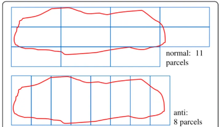
This test development start from the idea that in some cases it could be advantageous to orientate the parcels differently, not in the direction of length but in the direction of width (Fig. 6), so with a 90° rotation. The corresponding plan can be generated without modifying the second model, but simply by calling Procedure Make_Grid(“Contaminated_area”,3,30) instead of Proced-ure Make_Grid(“Contaminated_area”,30,3) for example. For simplification the test case containing parcels rotated by 90° is called“anti”.

The difficulty with this test is not to generate an “anti” plan, but to count how many parcels are generated per polygon feature in an“anti”scenario compared to the nor-mal scenario. The algorithm was modified in this respect.

The same data are used as for model 2.

An additional attribute should be created in the “ Con-tamination_aera” feature class called “feat_num” that store the feature number.

During the search cursor recursion:

1/a selection is done on the parcels of“Work_layer”that intersect the active polygon from“Contaminated area” 2/selection is switched

3/selected features deleted

4/a GetCount_management command is called to retrieve the number of parcel of selection

5/an arcpy.da.UpdateCursor command is used to update the“feat_num”for the activated FID.

Same data as for model 2 with the minor modifications cited above.

Offset effect testing: model development Description of the objectives

The model should move the features of clean-up parcel altogether following a grid pattern (so both in vertical and horizontal direction). The grid is oriented in the same way as the clean-up parcel feature class and the sampling distance of the grid is equal with a fifth of the parcel width. Each time the feature class is drifted the model counts how many features are located in the area of interest. The “get count” result with the smallest number of features shows the best offset to be applied.

the original area of interest is required to perform a selection based on intersection.

a new clean-up parcel feature class is necessary. It is similar to the one generated in model 1 with optimal

ori.>0

ori.<0

orig.= point 1&5 (x,y) point 2 ((x + length.cos(ori.),

y + length.sin(ori.))

point 3 (x – length.cos(-ori.) – width.sin(-ori.), y + length.sin(-ori.) – width.cos(-ori.))

point 4 (x + width.sin(ori.), y – width.cos(ori.))

point 2 (x – length.cos(-ori.), y + length..sin(-ori.)) point 3 (x + length.cos(ori.) + width.sin(ori.), y + length.sin(ori.) – width.cos(ori.))

point 4 (x – width.sin(-ori.), y – width..cos(-ori.))

Fig. 5Details of the coordinate calculations with vertices of the parcel and drawing method in createRectangleAtPoint procedure with the exact orientation cases

normal: 11 parcels

anti: 8 parcels

(7)

orientation but the reference area of interest differs (extended).

The extended reference area of interest is the original area of interest extended with a buffer zone of the parcel width. If this precaution is not implemented, the clean-up parcel extent is too lim-ited and for example an empty area appears on the left when x receives a positive drift.

1/The model should generate a new area of interest with a buffer of“length”size around the original area of interest.

2/Clean-up parcel feature class should be recreated based on the new target area (this is done in order not to have an empty area when the features will be shifted (maximal shift will be equal to parcel length)).

3/Calculate the shift values based on parcel width, length, orientation and store them in a three dimensional list.

4/All the features of this new clean-up feature class are shifted applying the offset values stored in the matrix (x,y). The grid x and y range are fixed at one-fifth of the parcel width.

5/Each time the feature class is shifted, a selection of the features intersecting with the original target area is done and the result of“getcount”is stored in a two dimensional list.

6/Unselect all features

7/Inverted shift is applied to set the feature back in place.

8/Next shift is applied, etc.

9/When all the shifting x,y values are passed, a search in the list value returns the smallest getcount.

10/From the minimal getcount, to retrieve the optimal x,y shift values.

11/Apply a final shift with the optimal x,y shift values.

Function_calculate_drift_matrix(length, width, orien-tation) This function returns a three dimensional matrix containing the shift coordinates corresponding to each point of the grid. The grid is oriented according to the parameter “orientation”. The step of the grid is width/5 both with “rows” and “columns”. For example if parcels are 30mx3m at 90°, there are 50 columns and 5 rows in the grid and the step is 3/5 m. This function has four parts for the four different orientations.

Funtion_shift_features(in_features, x_shift = None, y_shift = None) This function uses the arcpy.da

mod-ule’s UpdateCursor. By modifying the SHAPE@XY

token, it modifies the centroid of the feature and shifts

the rest of the feature to match. This function was avail-able online and usavail-able without changes, so it was simply copied [21].

Main procedure The procedure deals with the creation of the extended area of interest; appeals the two func-tions described above and deals with the searches in the list“getcount”.

Navigation lines model development Description of the objectives

The model should create a polyline feature class with navigation lines. The navigation lines should:

– be located in the middle of parcels,

– follow their length

Input:“clean-up parcel”shape file Output:“Navigation_lines”shape file Algorithm’s structure

Function_ExtractVerticesCoordinateFromFeature (input_feature_class) This function extracts the verti-ces’coordinates from a polygon feature class geometries and returns a two dimensional list storing the coordi-nates. SearchCursor method is employed on each row of the feature class. The result is appended to the list. Most of the script derives from the example of Reading poly-line or polygon geometries of ESRI resources help [22].

Function_CalculateMiddlePoints(list_corners)This func-tion receives the coordinates of the four corners of a rect-angle and returns the values of the coordinates of the two points located in the middle of the shortest sides.

Procedure_WriteaLine(point_1, point_2, layer) This procedure writes a polyline feature between two given points (coming from function_CalculateMiddlePoints) in the given layer. SearchCursor method is applied to enter new geometry.

Procedure_DrawNavigationLines(Ouput_Navigation_ Lines, Source_feature_class) This procedure makes use of the functions and procedures above to draw a new polyline feature class with the navigation lines. Create-featureclass_management method is used to create the output feature class.

(8)

Results and discussion

Clean-up parcel model with four orientations

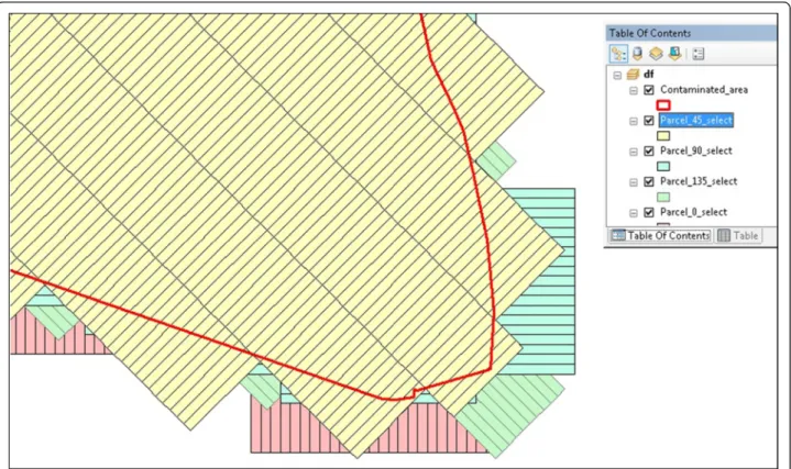
During its development the script was tested on a small feature extracted from the“Contaminated_area”shapefile.

Figure 7 shows an example of result with the four intermediary feature classes generated by the clean-up parcels model with 0°, 90°, 45° and 135° orientation, 3 m width and 30 m length on a sample of the contaminated area.

After correcting mistakes in the script the geo-processing model was applied to the whole“contaminated_area” sha-pefile. It resulted in very long geo-processing (more than 3 days to generate 0° and only a part of 45° orientation clean-up parcels layers).

Processing was voluntarily stopped before geo-processing was completed. This long calculation was caused:

1/by the extent and geometry of the target area (containing a lot of empty space where it was useless to have the geo-processing run),

2/by the huge number of parcels to generate (around 60,000); a direct effect of the extent of

contaminated_area,

3/by the procedure_Make_grid which is not efficient with geo-processing (a lot of unnecessary geo-processing is done during iteration outside of the area of interest).

To cope with these various problems the second test was run on the same data but split into 8 zones (11 sha-pefiles as zone 7 was split in four).

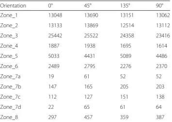
The number of features generated per zone with the four orientations is summarized in the Table 1. Smallest values are highlighted in green and highest in red back-ground. Combining the optimum orientation for each zone, the minimal number of feature in the clean-up plan reach 57,896.

At first we can observe a significant difference in the number of features obtained after geo-processing with different orientations. It appears the orientation of the parcel pattern is an important parameter to consider in optimizing planning.

Table 2 provides statistics per zone. First we calculated a classic measure of deviation ofσ/x̄(standard deviation divided by mean). As the number of entities vary signifi-cantly per sample (zone) and in order to have values of the same order it was necessary to divide deviation by mean. The deviation varies from 2 to 20 %. The second value provided in the table is more relevant in our opin-ion because it better expresses the important difference between the extremes and better pulls out the efficiency of the algorithm (subtraction of the maximum feature number with the minimum feature number divided by the maximum feature number and expressed in percent).

(9)

This value can be interpreted as the ability of the algo-rithm to“reduce”the number of parcels by x%. The fea-ture number reduction ranges from 5 to 38 %.

As a second conclusion the variations in the results can be very high (up to 38 %). This is definitely signifi-cant information for the planning strategy. Last, such a difference should be investigated and explained.

Figure 8 shows the geometry and size of the 8 zones in order to be able to cross the statistical results from Table 2 with spatial information. The following observation can be formulated: the smallest zones show bigger variances (re-ported to the mean) than the biggest zones.

Hypothesis 1: the reduced number of features is the cause of the bigger variance. Orientation matches more efficiently with smaller number of features because much of them are oriented in the same way. On the contrary when there are more features, their

orientation varies more and the efficiency of the model decreases.

Hypothesis 2: the cause for important variance is a scale effect because the model efficiency works with a border effect. On smaller areas the features could be smaller; the ratio boundary/area is more in favour of

the boundary compared to massive area and orientation becomes much more important.

After additional tests we could conclude that both hy-potheses seem valid. When comparing the results be-tween zone 4 that has two oriented features in the same direction and zone 7 a, b, c, d with small and long fea-tures; feature number decrease by 38 % with zone 7 whereas the feature number is only decreased by 17 % for zone 4.

In terms of practice with the preparation of“ Contami-nated_area”; in order to optimize the geo-processing, the user should pay attention to three things:

1/to prepare zones as small as possible in order to reduce empty areas (time consideration).

Table 1Number of features with the different orientations within the 8 zones

Orientation 0° 45° 135° 90°

Zone_1 13048 13690 13151 13062

Zone_2 13133 13869 12514 13112

Zone_3 25442 25522 24358 23416

Zone_4 1887 1938 1695 1614

Zone_5 5033 4431 5089 4486

Zone_6 2489 2795 2276 2370

Zone_7a 19 61 52 52

Zone_7b 147 165 205 203

Zone_7c 112 127 151 138

Zone_7d 22 65 61 64

Zone_8 297 457 359 387

Table 2Statistics with the 8 zones

Zone σ _̄x σ/x_̄ (Max-Min)/Max (in %)

1 305 13,238 2% 5 %

2 555 13,157 4 % 10 %

3 998 24,685 4 % 8 %

4 154 1784 9 % 17 %

5 349 4760 7 % 13 %

6 226 2483 9 % 19 %

7 81 411 20 % 38 %

8 66 375 18 % 35 %

(10)

2/to the extent possible have features with the same orientation inside one zone. If necessary, a zone should be split into several parts in order to ensure the features’general orientation is as similar as possible (example is 7 a, b, c, d).

3/to split feature if their geometry is complex. The result should be the creation of sub-features with sim-pler and oriented geometries.

In order to validate the presumptions mentioned above, the method was implemented on Zone 1 (Fig. 9) (where the algorithm showed the lowest efficiency) which was divided following the above recommenda-tions. New results are summarized in Table 3.

An additional reduction of 3.7 % could be reached by applying an appropriate cut with zone 1 compared to the previous result. This result prefigures the improve-ments that can possibly be reached with a modified algo-rithm (see model 2) and proper preparation of the

“Contaminated_area”layer.

Modification required and implemented in model 2

Regarding the reduction of geo-processing time, a test will be added inside the scripts implementing iteration. Before calling createRectangleAtPoint procedure an “IF” condition will be applied to check if the corner point (x,y) of the rectangle to be drawn falls into the area of interest (extended with a buffer zone of the parcel length). If x,y falls out no action will be taken, if it falls in then the rectangle will be written.

The orientation clearly appeared as a key parameter to control in order to optimize the remediation plan design. In our approach (which was exploratory) we decided to limit the number of orientation to 4 (with 0°, 45°, 90°

and 135°). In order to increase the efficiency of the model the optimal orientation could be identified with 1° accuracy. This means the algorithm should be im-proved to take the following actions:

1/isolate each individual polygon

2/calculate polygon’s orientation (with 1° accuracy) 3/apply a modified version of the clean-up parcel algorithm in order to design a clean-up plan with x° orientation for the feature considered.

With such an implementation, the optimized clean-up parcels are designed directly and it is no longer necessary to run the same script (clean-up parcel) four times with the four different orientations. So it would solve two issues: reducing the time processing and improving algo-rithm efficiency while reducing the number of parcel. This was applied with model 2 and the results are detailed in the paragraph below.

Dividing the contamination-area into subparts with homogenous orientation (and smaller geographic ex-tents) is the task of the user, it is not automatable.

Results of model with exact orientation

The run of model 2 lead to a final number of 55,066 par-cels compared to the 57,896 parpar-cels from the combin-ation of the optimal orientcombin-ation obtained per zone with model 1. This means a decrease of parcel number of 5 %. The model designed the clean-up plan (containing the 55,000+ parcels) in 3 h10. Figure 10 show an extract of the clean-up plan.

(a)

(b)

(c)

(d) (e) (f)

(g)

(h)

(i)

(j)(k) (m)

(l)

Fig. 9splitting of zone 1 into several parts

Table 3Counting of the number of features with the different orientation and the different sub-zones

Orientation 0° 45° 90° 135°

Zone_1a 887 1065 913 956

Zone_1b 507 605 588 593

Zone_1c 3076 3240 3089 3166

Zone_1d 459 527 483 453

Zone_1e 572 756 554 534

Zone_1f 3183 3449 3197 3216

Zone_1g 2037 2224 2052 2113

Zone_1h 1760 1836 1691 1770

Zone_1i 123 171 92 102

Zone_1j 166 170 102 161

Zone_1k 224 303 210 237

Zone_1l 71 84 61 73

Zone_1m 164 170 148 184

(11)

Results of 90° rotation testing

The “anti” clean-up plan results with a total of 65,165 parcels. This number is much higher than the one for normal plan. The reason is that in most case the normal orientation is optimal. Out of the 193 polygon features,

“anti” orientation is advantageous with 39 features (so 20 % of the feature number). With a combination of the

“anti” solution for the 39 cited features and the normal solution for the rest, the total parcel number reach 54,744. So in comparison with the normal solution, the parcel number could only be decreased by 0.5 %. We can conclude that model 3 showed very limited effi-ciency in our case study with the reduction of feature number. We decided not to go further with the development.

Results of shift testing

Model 4 testing showed very limited results with the re-duction of feature number. Only 1% difference with the number of features could be modelled. After further considerations, it seems that due to the irregular shape of the area of interest and the scale ratio, a shift is use-less because on average as parcels disappear on one border others appear on the opposite border. If the AOI is regular (rectangle for example) and the scale ratio much smaller (AOI area compared to parcel area), this tool could achieve significant results. In our case -a large scale industrial disaster with relatively large irregular areas- the tool shows limited efficiency; consequently we decided not to go further with the development.

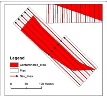
Draw navigation line model

Figures 11 and 12 below show the result of the Naviga-tion lines model. The 55,000+ navigaNaviga-tion lines were drawn in 0 h30.

The algorithm orients all the geometries of the lines in the same direction by default. Some additional algo-rithms development could be foreseen if it turns out that navigation requirement would need a pre-planned navi-gation direction and computation of the optimal order of visit. As the operation in the field constantly changes, this kind of development is not considered a priority at the moment.

In many places there is overlay between the navigation lines. This is a consequence of the overlay between the clean-up parcels (visible in Fig. 9). The draw navigation live model should be improved in order to remove those overlays.

Fig. 10Extract of the clean-up plan

Fig. 11Navigation lines feature class generated by the navigation

(12)

Improvements and future development

Improvement can be done with the algorithm efficiency by strictly constraining iterations to inside the boundaries of the contaminated area in order to avoid parcel creation (and time waste) out of the pollution features areas.

Contaminated area datasets with varying shapes should be tested to assess the efficiency of the geo-processing models we designed with other type of pollution coverage (and shapes). There could be some situations where ineffi-cient models (drift, parcel rotation) could become advantageous.

As mentioned in paragraph 7.5, on many places where contamination features are close to each other, the clean-up parcels are overlaying which in the end results with overlapping navigation lines. The next development should consider if it is worth correcting the clean-up parcel layer or either the navigation line layer with cut-ting the overlaying parts.

Inspired from the literature about“coverage path plan-ning” [14, 15–17], it would be interesting to consider if capacitated vehicle routing problem models could bring added value in the remediation work, in the case of soil excavation by heavy equipment.

Conclusions

First we demonstrated that among four different plans with four different orientations, one plan comprised less features and constituted an optimized version compared to the others. In return this showed how important it is to consider the source feature orientation for the orientation

of the features of the clean-up plan. Additionally we demonstrated that improper orientation can lead to an important increase of the number of clean-up parcels, particularly if feature has a complex shape or if the source feature/parcel feature scale ratio is low. We have demonstrated that the best modelling approach consist in processing each contaminated feature separately, computing its orientation and applying the same orien-tation to the clean-up plan. The different tests also highlighted the importance of the dataset preparation, by cutting complex feature into sub-features with a unique orientation. Last but not least we demonstrated that automatic planning can be achieved both with the

clean-up parcels and the navigation lines on a 4 km2

impacted area, with 55,000+ features for each generated in an approximate total time of 3 h40.

Endnotes 1

from aerial survey and remote sensing processing methods

2

ex-situ remediation is opposed to on-site remediation and requires the excavation of soil and its transportation out of the site.

Competing interests

The authors declare that they have no competing interests.

Authors’contributions

GL carried out the main research based on his thesis work realised at the Doctoral School of Military Engineering at the National University of Public Service in Budapest and the Research Institute of Remote Sensing and Rural Development in Gyöngyös. GL conceived the study, developed the algorithm, tested the algorithms and drafted the manuscript. JS and CsL participated in review of the manuscript and made proposals for its further development. All authors read and approved the final manuscript.

Received: 8 March 2016 Accepted: 27 April 2016

References

1. Anton AD, Klebercz O, Magyar A, Burke IT, Jarvis AP, Gruiza K, Mayes WM. Geochemical recovery of the Torna–Marcal river system after the Ajka red mud spill, Hungary. Environ Sci Processes Impacts. 2014;2014(16):2677_–85. doi:10.1039/C4EM00452C. http://pubs.rsc.org/en/content/articlepdf/2014/ em/c4em00452c. Accessed 2 May 2016.

2. Schweitzer F. Channel regulation of Torna stream to improve environmental conditions in the vicinity of red sludge reservoirs at Ajka, Hungary. Hungarian Geogr Bull. 2010;59(4):347–59. http://epa.oszk.hu/02500/02541/00008/ pdf/EPA02541_hungeobull_2010_4_347-359.pdf. Accessed 2 May 2016. 3. Berke J, Bíró T, Burai P, Kováts LD, Kozma-Bognár V, Nagy T, Tomor T,

Németh T. Application of remote sensing in the red mud environmental disaster in Hungary. Carpathian J Earth Environ Sci. 2013;8(2):49–54. 4. Burai P, Smailbegovic A, Cs L, Berke J, Tomor T, Bíró T. Preliminary analysis

of red mud spill based on aerial imagery. Acta Geographica Debrecina Landscape Environ Ser. 2011;5(I):47_–57.

5. Driscoll A. GIS Applications in Site Remediation. 2004. http://www.edc.uri. edu/nrs/classes/nrs409/509_2004/Driscoll.pdf. Accessed 2 May 2016. 6. Franco C, Delgado J, Soares A. Impact Analysis and Sampling Design in The

Pollution monitoring Process of The Aznalcollar Accident using Geostatistical Methods. In: The International Archives of the

Photogrammetry, vol. XXXV, Part B7. Istanbul: Remote Sensing and Spatial Information Sciences; 2004. p. 373–8.

7. Guyard C. Dépollution des sols et nappes : un marché sous pression. L_’eau, l’industrie, les nuisances. 2013;359:23–40.

(13)

8. Hellawell EE, Kemp AC, Nancarrow DJ. A GIS raster technique to optimize contaminated soil removal. Eng Geol. 2001;60(1_–4):107_–16.

9. Lindsay J, Simon T, Graettinger G. Application of USEPA FIELDS GIS technology to support Remediation of Petroleum Contaminated Soils on the Pribilof Islands, Alaska. 2nd_{Biennial Coastal GeoTools Conference, Charleston, SC,} January 8_–11. 2001. http://webapp1.dlib.indiana.edu/virtual_disk_library/index. cgi/5293706/FID2516/pdf_files/ps_abs/lindsayj.pdf. Accessed 1 Jul 2015. 10. Mathieu JB, Garcia V, Garcia M, Rabaute A. SoilRemediation: a plugin and

workflow in Gocad for managing environmental data and modeling contaminated sites. Gocad Meeting, Nancy June 2_–5, 2009.

11. Webster I, Ciccolini L. Solving contaminated site problems cost effectively: plan, use geographical systems (GIS) and execute. http://www.

projectnavigator.com/downloads/webster_ciccolini_solving_contaminated_ sites_04.09.02.pdf. Accessed 1 Jul 2015.

12. Dukukovíc J, Stanojevic M, Vranes S. GIS Based Decision Support Tool for Remediation Technology Selection. Proceedings of the 5th IASME/WSEAS Int. Conference on Heat Transfer, Thermal Engineering and Environment, Athens, Greece, August 25_–27, 2007.

13. Interstate Technology & Regulatory Council (ITRC). Remediation Process Optimization: Identifying Opportunities for Enhanced and More Efficient Site Remediation. 2004.

14. Conesa-Muñoz J, Pajares G, Ribeiroa A. Mix-opt: A new route operator for optimal coverage path planning for a fleet in an agricultural environment. Expert Syst Appl. 2016;54(2016):364–78.

15. Fergusson D, Likhachev M, Stentz A. A Guide to Heuristic-based Path Planning. Proceedings of the International Workshop on Planning under Uncertainty for Autonomous Systems, International Conference on Automated Planning and Scheduling (ICAPS), June, 2005. http://www.cs. cmu.edu/~maxim/files/hsplanguide_icaps05ws.pdf. Accessed 2 May 2016. 16. Driscoll TM._“Complete coverage path planning in an agricultural

environment”. Graduate Theses and Dissertations. Paper 12095. 2011. http://lib.dr.iastate.edu/cgi/viewcontent.cgi?article=3053&context=etd. Accessed 2 May 2016.

17. Hameed IA, la Cour-Harbob A, Osena OL. Side-to-side 3D coverage path planning approach for agricultural robots to minimize skip/overlap areas between swaths. Robot Auton Syst. 2016;76:36–45.

18. Hameed IA. Intelligent coverage path planning for agricultural robots and autonomous machines on three-dimensional terrain. J Intell Robot Syst. 2013;74(3):965–83.

19. Global remediation technologies. MAPPING & MODELING http://grtusa.com/ services/mapping-modeling/. Accessed 1 Jul 2015.

20. ArcGIS Help 10.1/Extent (Arcpy). http://gis.stackexchange.com/questions/ 72895/how-to-obtain-an-extent-of-a-whole-shapefile. Accessed 1 Jul 2015. 21. ArcPy Café/Shifting features. https://arcpy.wordpress.com/2012/11/15/

shifting-features/. Accessed 2 May 2016.

22. ArcGIS Help 10.1/Reading geometries. http://resources.arcgis.com/en/help/ main/10.1/index.html#/Reading_geometries/002z0000001t000000/. Accessed 1 Jul 2015.