The five-loop beta function of Yang-Mills theory with fermions

JHEP02(2017)090

Received: January 12, 2017

Accepted: February 9, 2017

Published: February 17, 2017

The five-loop beta function of Yang-Mills theory with

fermions

F. Herzog,a B. Ruijl,a,b T. Ueda,a J.A.M. Vermaserena and A. Vogtc

a_{Nikhef Theory Group,}

Science Park 105, 1098 XG Amsterdam, The Netherlands

b_{Leiden Centre of Data Science, Leiden University,}

Niels Bohrweg 1, 2333 CA Leiden, The Netherlands

c_{Department of Mathematical Sciences, University of Liverpool,}

Liverpool L69 3BX, United Kingdom

E-mail: [email protected],[email protected],[email protected],

[email protected],[email protected]

Abstract: _{We have computed the five-loop corrections to the scale dependence of the}

renormalized coupling constant for Quantum Chromodynamics (QCD), its generalization to non-Abelian gauge theories with a simple compact Lie group, and for Quantum Elec-trodynamics (QED). Our analytical result, obtained using the background field method, infrared rearrangement via a new diagram-by-diagram implementation of the R∗ _operation

and theForcer_{program for massless four-loop propagators, confirms the QCD and QED}

results obtained by only one group before. The numerical size of the five-loop corrections is briefly discussed in the standard MS scheme for QCD withn_f flavours and for pure SU(N) Yang-Mills theory. Their effect in QCD is much smaller than the four-loop contributions, even at rather low scales.

Keywords: _{Perturbative QCD, Renormalization Group}

JHEP02(2017)090

Contents

1 Introduction 1

2 Theoretical framework and calculations 2

2.1 Background field method 2

2.2 Group notations 4

2.3 The R∗_{-operation 4}

2.4 Diagram computations and analysis 6

3 Results and discussion 7

4 Summary and outlook 11

A Tensor reduction 13

1 Introduction

The scale dependence (‘running’) of the renormalized coupling constantα_iis a fundamen-tal property of an interacting quantum field theory. In renormalization-group improved perturbation theory, the beta function governing this dependence can be written as

da

dlnµ2 =β(a) =− ∞

X

n=0

βnan+2, a= α_i(µ)

4π (1.1)

whereµis the renormalization scale. The determination of the (sign of the) leading one-loop coefficientβ0 [1–5], soon followed by the calculation of the two-loop correctionβ1 [6,7], led

to the discovery of the asymptotic freedom of non-Abelian gauge theories and thus paved the way for establishing QCD as the theory of the strong interaction. The renormalization-scheme dependent three-loop (next-to-next-to-leading order, N2LO) and four-loop (next-to-next-to-next-to-leading order, N3_{LO) coefficientsβ}

2andβ3were computed in refs. [9,10]

and [11,12] in minimal subtraction schemes [13,14] of dimensional regularization [15,16]. In the past years, the N2LO accuracy has been reached for many processes at high-energy colliders. N3_{LO corrections have been determined for structure functions in inclusive}

deep-inelastic scattering (DIS) [17,18] and for the total cross section for Higgs-boson pro-duction at hadron colliders [19, 20]. Some moments of coefficient functions for DIS have recently been computed at N4_{LO [21]. Reaching this order would virtually remove the}

un-certainty due to the truncation of the series of massless perturbative QCD in determinations of the strong coupling constantαs from the scaling violations of structure functions in DIS.

JHEP02(2017)090

required more than a year of computations on a decent number of multi-core workstations in a highly non-trivial theoretical framework. These critical parts have neither been extended to a general gauge group nor validated by a second independent calculation so far.

In the present article we address this issue and present the five-loop beta function for a general simple gauge group. Unlike the calculations in refs. [4–12], we have employed the background field method [26,27], which we found to be more efficient — in validation calculations of theForcer_{program [28–30] of the four-loop renormalization of Yang-Mills}

theories to all powers of the gauge parameter — than the computation of two propagators and a corresponding vertex. This method and other theoretical and calculational issues, in particular a new implementation [31] of the R∗ _{operation [32–35] for massless}

propagator-like diagrams, are addressed in section 2; the details of the required tensor reduction can be found in the appendix. We present and discuss our result in section 3, and briefly summarize our findings in section 4.

2 Theoretical framework and calculations

In this section we briefly review the background-field formalism and theR∗ _{operation. We}

further define our notations for group invariants, and we give an overview of our calculation.

2.1 Background field method

A convenient and efficient method to extract the Yang-Mills beta function is to make use of the background field. We will briefly review this formalism. A convenient starting point is the Lagrangian of Yang-Mills theory coupled to fermions in a non-trivial (often the fundamental) representation of the gauge group, the theory for which we will present the 5-loop beta-function in the next section.

The Lagrangian of this theory can be decomposed as

L_YM+FER=L_CYM+L_GF+L_FPG+L_FER. (2.1) Here the classical Yang-Mills Lagrangian (CYM), a gauge-fixing term (GF), the Faddeev-Popov ghost term (FPG) and the fermion term (FER) are given by

L_CYM =−1

4F a

µν(A)Faµν(A),

L_GF =−1

2ξ(G a₎2_,

L_FPG =−η†_a∂µD_µab(A)η_b, L_FER =X

i,j,f ¯

ψif(i /Dij(A)−mfδij)ψjf. (2.2)

In the fermion term the sum goes over colours i, j, and nf flavours f, and we use the standard Feynman-slash notation. The field strength is given by

F_µνa (A) =∂µAaν−∂νAaµ+gfabcAbµAcν (2.3) and the covariant derivatives are defined as

Dab_µ(A) =δab∂µ−gfabcAcµ,

JHEP02(2017)090

The conventions associated to the generatorsTaand structure constants fabc of the gauge group will be explained in section2.2. The gauge-fixing term depends on making a suitable choice for Ga_{, which is usually taken as G}a_=∂µ_Aa

µ.

The background-field Lagrangian is derived by decomposing the gauge field as

Aa_µ(x) =B_µa(x) + ˆAa_µ(x), (2.5)

where Ba_µ(x) is the classical background field while ˆAa_µ(x) contains the quantum degrees of freedom of the gauge field Aa

µ(x). The background-field Lagrangian is then written as

L_BYM+FER =L_BCYM+L_BGF+L_BFPG+L_BFER. (2.6)

L_BCYM and L_BFER are derived simply by substituting eq. (2.5) into the corresponding terms in the Yang-Mills Lagrangian. However a clever choice exists [26, 27] for the ghost and gauge fixing terms, which allows this Lagrangian to maintain explicit gauge invariance for the background field B_µa(x), while fixing only the gauge freedom of the quantum field

ˆ

Aa

µ(x). The gauge fixing then uses instead

Ga=Dab_µ(B) ˆAµ_b , (2.7)

while the ghost term is given by

L_BFPG=−η_a†Dab;µ(B)Dbc_µ(B+ ˆA)ηc. (2.8) The Lagrangian L_BYM+FER then gives rise to additional interactions which are different from the normal QCD interactions of the quantum field ˆAa_µ(x) also contain interactions of

B_µa(x) with all other fields.

A remarkable fact is found when considering the renormalization of this Lagrangian. Indeed it turns out, see e.g., [26,27], that the coupling renormalization, g →Zgg, which determines the beta function, is directly related to the renormalization of the background field,B →BZB, via the identity:

Zg p

ZB = 1. (2.9)

When working in the Landau gauge, the only anomalous dimension needed in the back-ground field gauge formalism is then the beta function. However in the Feynman gauge the gauge parameterξ requires the renormalization constantZξ — which equals the gluon field renormalization constant — but only to one loop lower. In turn this allows one to extract the beta function from the single equation

ZB(1 + ΠB(Q2;Zξξ, Zgg)) = finite, (2.10)

with

Πµν_B(Q;Zξξ, Zgg) = (Q2gµν−QµQν) ΠB(Q2;Zξξ, Zgg) (2.11) where Πµν_B(Q2_{;ξ, g) is the bare self energy of the background field. This self-energy is}

computed by keeping the fields B external while the only propagating fields are ˆA, η and

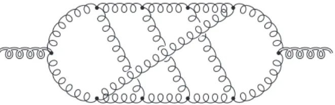
ψ. A typical diagram which contributes to ΠB(Q2;ξ, g) is given in figure1.

JHEP02(2017)090

double lines represent the background field. The presence of the 10 purely gluonic vertices creates a large expression after the substitution of the Feynman rules.

2.2 Group notations

In this section we introduce our notations for the group invariants appearing in the results of the next section. Ta are the generators of the representation of the fermions, and fabc

are the structure constants of the Lie algebra of a compact simple Lie group,

TaTb−TbTa=ifabcTc. (2.12)

The quadratic Casimir operators CF and CA of the N-dimensional fermion and the NA -dimensional adjoint representation are given by [TaTa]ik = CFδik andfacdfbcd = CAδab, respectively. The trace normalization of the fermion representation is Tr(Ta_Tb_{) = T}

Fδab. At L ≥ 4 loops also quartic group invariants enter the beta function. These can be expressed in terms of contractions of the totally symmetric tensors

d_Fabcd = 1 6Tr(T

a_Tb_Tc_Td _{+ fivebcdpermutations),}

d_Aabcd = 1 6Tr(C

a_Cb_Cc_Cd_{+ fivebcdpermutations). (2.13)}

Here the matrices [Ca]bc = −ifabc are the generators of the adjoint representation. It should be noted that in QCD-like theories without particles that are colour neutral, Furry’s theorem [36] prevents the occurrence of symmetric tensors with an odd number of indices. For the fermions transforming according to the fundamental representation and the standard normalization of the SU(N) generators, these ‘colour factors’ have the values

TF = 1

2, CA=N , CF =

NA 2N =

N2₋₁

2N ,

d_Aabcdd_Aabcd NA

= N

2_(N2_{+ 36)}

24 ,

dabcd F dAabcd

NA

= N(N

2_{+ 6)}

48 ,

dabcd F dFabcd

NA

= N

4_−6N2₊₁₈

96N2 . (2.14)

The results for QED (i.e., the group U(1)) are obtained for CA = 0, dAabcd = 0, CF = 1, TF = 1, dabcdF = 1, and NA = 1. For a discussion of other gauge groups the reader is referred to ref. [11].

2.3 The R∗_-operation

JHEP02(2017)090

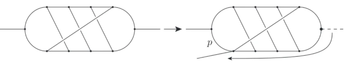
Figure 2. One external line is moved to create a topology that can be integrated. Here we do this for the diagram of figure1. One should take into account that there can be up to 5 powers of dot products in the numerator, causing many subdivergences. Furthermore, the double propagator that remains on the right can introduce infrared divergences. After the subdivergences have been subtracted, the integral over p can be performed and the remaining four-loop topology can be handled by theForcer_program.

it is beyond current computational capabilities to calculate the required five-loop propa-gator integrals directly. The main obstacle preventing such an attempt is the difficulty of performing the required integration-by-parts (IBP) reductions.

Fortunately the problem can be simplified via the use of the R∗_{-operation. The R}∗

-operation [32–35] is a subtraction operation capable of rendering any propagator integral finite by adding to it a number of suitable subtraction terms. The subtraction terms are built from potentially high rank tensor subgraphs of the complete graph, whose tensor reduction requires involved methods which we present in appendix A. Via the procedure ofIR-rearrangement, these subtraction terms can subsequently be related to simpler prop-agator integrals. The IR-rearranged integral is, in general, any other propprop-agator integral obtained from the original one by rerouting the external momentum in the diagram. This is illustrated in figure2.

For integrals whose superficial degree of divergence (SDD) is higher than logarithmic, the SDD is reduced by differentiating it sufficiently many times with respect to its external momenta, before IR-rearranging it.

The upshot of this procedure is that the IR-rearranged propagator integrals can be chosen to be carpet integrals, which correspond to graphs where the external lines are connected only by a single propagator. A carpet integral of L loops can be evaluated as a product of an (L−1) loop tensor propagator integral times a known one-loop tensor integral. In the case of the five-loop beta function this means that we can effectively evaluate the poles of all five-loop propagator integrals from the knowledge of propagator integrals with no more than four loops. A sketch of the R∗_{-operation to compute the}

superficial divergence of a 3-loop diagram is shown below:

!

sup

=

!

sup

=

K −K

!

−

!

sup

!

JHEP02(2017)090

where sup denotes the superficial divergence, and K isolates the pole of a Laurent series inǫ. As can be seen, the R∗_{-operation is recursive, since the same procedure needs to be}

applied to compute the superficial divergence of each counterterm.

The Forcer_{program [29,30], written in the}Form_{language, is capable to efficiently}

compute the subtraction terms. It reduces four-loop propagator integrals to simpler known ones by integrating two-point functions, and by applying parametrically solved IBP reduc-tion rules to eliminate propagators. We have automated the R∗_{-operation in a fast Form}

program, capable of performing the subtraction of propagator integrals with arbitrary ten-sorial rank. Having interfaced the Forcer_{program with theR}∗ _{program we were able to}

compute the poles of all integrals entering the five-loop background field self-energy. The algorithms and details of our implementation of the R∗_{-operation follow to some degree}

the ideas which were presented in the literature (see e.g., [32–35, 37, 38]), however we have generalized certain notions in order to deal with arbitrary tensor integrals and their associated ultraviolet and infrared divergences. These generalizations are subtle and will be presented elsewhere [31].

2.4 Diagram computations and analysis

The Feynman diagrams for the background propagator up to five loops have been generated using QGRAF [39]. They have then been heavily manipulated by aForm_{[40–42] program}

that determines the topology and calculates the colour factor using the program of ref. [43]. Additionally, it merges diagrams of the same topology, colour factor, and maximal power of

n_f into meta diagrams for computational efficiency. Integrals containing massless tadpoles or symmetric colour tensors with an odd number of indices have been filtered out from the beginning. Lower-order self-energy insertions have been treated as described in ref. [44]. In this manner we arrive at 2 one-loop, 9 two-loop, 55 three-loop, 572 four-loop and 9414 five-loop meta diagrams.

The diagrams up to four loops have been computed earlier to all powers of the gauge parameter using theForcer_{program [28–30]. For the time being, our five-loop}

computa-tion has been restricted to the Feynman gauge, ξF = 1−ξ = 0. An extension to the first power inξF would be considerably slower; the five-loop computation for a generalξ would be impossible without substantial further optimizations of our code. Instead of by vary-ingξ, we have checked our computations by verifying the relation QµQνΠ_Bµν = 0 required by eq. (2.11). This check took considerably more time than the actual determination ofβ4.

The five-loop diagrams have been calculated on computers with a combined total of more than 500 cores, 80% of which are older and slower by a factor of almost three than the latest workstations. One core of the latter performs a ‘raw-speed’Form_{benchmark, a}

four-dimensional trace of 14 Dirac matrices, in about 0.02 seconds which corresponds to 50 ‘form units’ (fu) per hour. The total CPU time for the five-loop diagrams was 3.8·107 seconds which corresponds to about 2.6·105 _{fu on the computers used. TheTFormparallelization}

efficiency for single meta diagrams run with 8 or 16 cores was roughly 0.5; the whole calculation ofβ4, distributed ‘by hand’ over the available machines, finished in three days.

For comparison, the corresponding R∗ _{computation for ξ}

JHEP02(2017)090

function to order ξ_F1 by a totally different method in ref. [11]. The computation with the

Forcer_{program at four and fewer loops is much faster, in fact fast enough to comfortably}

demonstrate the full three-loop renormalization of QCD in 10 minutes on a laptop during a seminar talk [45].

The determination ofZBfrom the unrenormalized background propagator is performed by imposing, order by order, the finiteness of its renormalized counterpart. The beta function can simply be read off from the 1/ε coefficients of ZB. If the calculation is performed in the Landau gauge, the gauge parameter does not have to be renormalized. In ak-th order expansion about the Feynman gauge at five loops, theL <5 loop contributions are needed up toξ_F5−L. The four-loop renormalization constant for the gauge parameter is not determined in the background field and has to be ‘imported’. In the presentk= 0 case, the terms already specified in ref. [12] would have been sufficient had we not performed the four-loop calculation to all powers of ξF anyway.

3 Results and discussion

Before we present our new result, it may be convenient to recall the beta function (1.1) up to four loops [4–12] in terms of the colour factors defined in section2,

β0 =

11 3 CA−

4

3 TFnf, (3.1)

β1 =

34 3 C

2

A − 20

3 CATFnf−4CF TFnf, (3.2)

β2 = 2857

54 C 3 A − 1415 27 C 2

ATF nf − 205

9 CFCATF nf + 2C

2

FTFnf

+ 44 9 CFT

2

F nf2+ 158

27 CAT

2

F nf2, (3.3)

β3 =CA4

150653 486 −

44 9 ζ3

+d

abcd A dAabcd

NA

−80

9 + 704

3 ζ3

+C_A3T_Fn_f

−39143

81 + 136

3 ζ3

+C_A2C_FT_F n_f

7073

243 − 656

9 ζ3

+C_AC_F2T_Fn_f

−4204

27 + 352

9 ζ3

+d abcd F dAabcd

NA n_f 512 9 − 1664

3 ζ3

+ 46C_F3T_F n_f +C_A2T_F2n_f2

7930

81 + 224

9 ζ3

+C_F2T_F2n_f2

1352

27 − 704

9 ζ3

+C_AC_FT_F2n_f2

17152

243 + 448

9 ζ3

+d abcd F dFabcd

NA n_f2

−704

9 + 512

3 ζ3

+ 424 243CAT

3

F nf3 + 1232

243 CF T

3

F nf3 , (3.4)

JHEP02(2017)090

of the scaleµ. In the same notation and scheme, the five-loop contribution reads

β4 =CA5

_8296235

3888 − 1630

81 ζ3+ 121

6 ζ4− 1045

9 ζ5

+d abcd A dAabcd

NA C_A −514 3 + 18716

3 ζ3−968ζ4− 15400

3 ζ5

+C_A4T_Fn_f

−5048959

972 + 10505

81 ζ3− 583

3 ζ4+ 1230ζ5

+C_A3C_FT_Fn_f

8141995

1944 + 146ζ3+ 902

3 ζ4− 8720

3 ζ5

+C_A2C_F2T_Fn_f

−548732

81 − 50581

27 ζ3− 484

3 ζ4+ 12820

3 ζ5

+C_AC_F3T_F n_f

3717 + 5696 3 ζ3−

7480 3 ζ5

−C_F4T_Fn_f

₄₁₅₇

6 + 128ζ3

+d abcd A dAabcd

NA

T_F n_f

₉₀₄

9 − 20752

9 ζ3+ 352ζ4+ 4000

9 ζ5

+d abcd F dAabcd

NA

C_An_f

11312

9 −

127736

9 ζ3+ 2288ζ4+ 67520

9 ζ5

+d abcd F dAabcd

NA

C_Fn_f

−320 +1280 3 ζ3+

6400 3 ζ5

+C_A3T_F2n_f2

843067 486 +

18446 27 ζ3−

104 3 ζ4−

2200 3 ζ5

+C_A2C_FT_F2n_f2

5701

162 + 26452

27 ζ3− 944

3 ζ4+ 1600

3 ζ5

+C_F2C_AT_F2n_f2

31583

18 − 28628

27 ζ3+ 1144

3 ζ4− 4400

3 ζ5

+C_F3T_F2n_f2

−5018

9 − 2144

3 ζ3+ 4640

3 ζ5

+d abcd F dAabcd

NA

T_F n_f2

−3680

9 + 40160

9 ζ3−832ζ4− 1280

9 ζ5

+d abcd F dFabcd

NA

C_An_f2

−7184

3 + 40336

9 ζ3−704ζ4+ 2240

9 ζ5

+d abcd F dFabcd

NA

C_Fn_f2

4160

3 + 5120

3 ζ3− 12800

3 ζ5

+C_A2T_F3n_f3

−2077

27 − 9736

81 ζ3+ 112

3 ζ4+ 320

9 ζ5

+C_AC_FT_F3n_f3

−736

81 − 5680

27 ζ3+ 224

3 ζ4

+C_F2T_F3n_f3

−9922

81 + 7616

27 ζ3− 352

3 ζ4

+d abcd F dFabcd

NA

T_F n_f3

3520

9 − 2624

3 ζ3+ 256ζ4+ 1280

3 ζ5

+C_AT_F4n_f4

916 243−

640 81 ζ3

−C_FT_F4n_f4

856 243+

128 27 ζ3

JHEP02(2017)090

ζ5 ∼= 1.036927755. As expected from the lower-order and QED results, higher values of the

zeta function do not occur despite their occurrence in the results for individual diagrams; for further discussions see refs. [23,46].

Inserting the group factors of SU(3) as given in eq. (2.14) leads to theQCDresults

β0 = 11−

2

3nf, β1= 102− 38

3 nf,

β2 =

2857 2 −

5033 18 nf +

325 54 n

2

f ,

β3 =

149753

6 + 3564ζ3+nf

−1078361

162 − 6508

27 ζ3

+n_f2

50065

162 + 6472

81 ζ3 + 1093 729 n 3 f (3.6) and

β4= 8157455

16 +

621885 2 ζ3−

88209

2 ζ4−288090ζ5 +n_f

−336460813

1944 −

4811164 81 ζ3+

33935 6 ζ4+

1358995 27 ζ5

+n_f2

25960913 1944 +

698531 81 ζ3−

10526 9 ζ4−

381760 81 ζ5

+n_f3

−630559

5832 − 48722

243 ζ3+ 1618

27 ζ4+ 460

9 ζ5

+n_f4

1205 2916−

152 81 ζ3

. (3.7)

In truncated numerical form β3 andβ4 are given by

β3 ∼= 29242.964−6946.2896nf + 405.08904nf2+ 1.499314nf3, (3.8) β4 ∼= 537147.67−186161.95nf + 17567.758nf2−231.2777nf3−1.842474nf4. (3.9)

In contrast to β0, β1, and β2, which change sign at about nf = 16.5, 8.05, and 5.84 respectively, β3 and β4 are positive (except at very large n_f for β4), but have a (local)

minimum atn_f ≃8.20 andn_f ≃6.07.

The corresponding analytical result for QED, in the same renormalization scheme(s) but defined without the overall minus sign in eq. (1.1) is given by

β0 =

4

3nf, β1 = 4nf, β2 =−2nf − 44

9 n

2

f ,

β3 =−46nf +nf2

760 27 −

832 9 ζ3

−1232 243 n 3 f (3.10) and

β4 =nf

4157

6 + 128ζ3

+n_f2

−7462

9 −992ζ3+ 2720ζ5

+n_f3

−21758

81 + 16000

27 ζ3− 416

3 ζ4− 1280

3 ζ5

+n_f4

856 243+

128 27 ζ3

JHEP02(2017)090

The (corresponding parts of the) results (3.5), (3.7) and (3.11) are in complete agreement with the findings of refs. [22–25]. Consequently, eq. (3.11) also agrees with the result for QED atn_f = 1, which was obtained in ref. [47] somewhat earlier than the general result [23]. As already noted in ref. [22], the five-loopQCDcoefficient of the beta function is rather small [ recall that we use a convenient but very small expansion parameter in eq. (1.1)]. Indeed, for the physically relevant values ofn_f the expansion in powers ofαs reads

e

β(αs, nf = 3) = 1 + 0.565884αs+ 0.453014αs2+ 0.676967αs3+ 0.580928αs4,

e

β(αs, nf = 4) = 1 + 0.490197αs+ 0.308790αs2+ 0.485901αs3+ 0.280601αs4,

e

β(αs, nf = 5) = 1 + 0.401347αs+ 0.149427αs2+ 0.317223αs3+ 0.080921αs4,

e

β(αs, nf = 6) = 1 + 0.295573αs−0.029401αs2+ 0.177980αs3+ 0.001555αs4, (3.12)

where βe≡ −β(as)/(as2β0) has been re-expanded in powers of αs = 4π as. Clearly there is

no sign so far of a possible divergence of the perturbation series for this quantity.

In order to further illustrate then_f-dependent convergence (or the lack thereof) of the beta function of QCD, we introduce the quantity

b

α_s(n)(n_f) = 4π

βn−1(nf) 4βn(n_f)

. (3.13)

Recalling the normalization (1.1) of our expansion parameter,α_bs(n)(n_f) represents the value

of αs for which the n-th order correction is 1/4 of that of the previous order. Therefore, αs<∼αbs(n)(n_f) defines (somewhat arbitrarily due to the choice of a factor of 1/4) a region of

fast convergence of β(αs, n_f). Obviously, the absolute size of then-th and (n−1)-th order

effects are equal for αs = 4αb(n)(nf). Thus the quantity (3.13) also indicates where the expansion appears not to be reliable anymore, αs>∼4αbs(n)(n_f), for a given value of n_f that

is not too close to zeros or minima of the coefficientsβn−1 andβn.

It is interesting to briefly study the N-dependence of the convergence behaviour for the case of SU(N) gauge theories. For our brief illustration we confine ourselves to pure Yang-Mills theory, n_f = 0, and consider

b

α_YM(n)(N) = 4π N

βn−1(N)

4βn(N)

, (3.14)

where the factor N compensates the leading large-N dependence Nn+1 _{of β}

n, i.e., the parameter that needs to be small in SU(N) Yang-Mills theory is notα_YM butN α_YM.

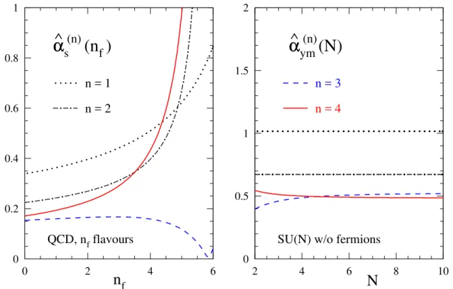
The quantities (3.13) and (3.14) are displayed in the left and right panel of figure 3, respectively. The behaviour of α_bs(n) at the upper end of the n_f range shown in the figure

is affected by the zeros and minima of the coefficients βn >0 mentioned below eq. (3.9). The N-dependence of α_bYM for pure Yang-Mills theory, where only terms with Nn+1 and Nn−1 _{enter β}

n (the latter only atn≥4 via d_Aabcdd_Aabcd/NA, cf. eq. (2.14) above), is rather weak. With only the curves up to four loops, one might be tempted to draw conclusions from the shrinking of the ‘stable’ αs region from NLO to N2LO and from N2LO to N3LO

JHEP02(2017)090

0 0.2 0.4 0.6 0.8 1

0 2 4 6

n

α

∧

s

α

∧

(n)

(n

)

n = 1

n = 2

QCD, n

flavours

N

α

∧

ym

(N)

α

∧

(n)

n = 3

n = 4

SU(N) w/o fermions

0 0.5 1 1.5 2

2 4 6 8 10

Figure 3. The values (3.13) and (3.14) of the coupling constants of QCD (left) and pure SU(N) Yang-Mills theory (right) for which the absolute size of the Nn_{LO contribution to the beta function}

is a quarter of that of the Nn₋1

LO term forn= 1, 2, 3 (dashed curves) and 4 (solid curves).

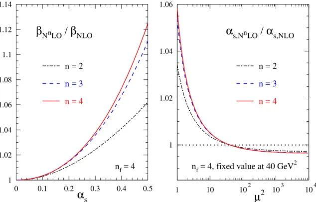
Finally, we briefly illustrate the cumulative effect of the orders up to N4LO on the beta function of QCD and the scale dependence of the strong coupling constantαs in figure 4.

For this illustration we setn_f = 4 and choose, in order to only show the differences caused by the running of the coupling, an order-independent value of αs = 0.2 at µ2 = 40 GeV2.

A realistic order dependence of αs at this scale, as determined from the scaling

viola-tions in DIS, would be 0.208, 0.201, 0.200, and 0.200 at NLO, N2_{LO, N}3_{LO, and N}4_LO,

respectively [17].

Adding the N4LO contributions changes the beta function by less than 1% atαs = 0.47

for n_f = 4 and at αs = 0.39 for n_f = 3; the corresponding values at N3LO are 0.29 and

0.26. The N4LO effect on the values ofαsas shown in figure4are as small as 0.08% (0.4%)

at µ2 _{= 3 GeV}2 _{(1 GeV}2_{); the corresponding N}3_{LO corrections are 0.5% (2%). Of course}

these results do not preclude sizeable purely non-perturbative corrections, but it appears that the perturbative running ofαs is now fully under control for all practical purposes.

4 Summary and outlook

The five-loop (next-to-next-to-next-to-next-to-leading order, N4_{LO) coefficient β}

4 of the

JHEP02(2017)090

1 1.02 1.04 1.06 1.08 1.1 1.12 1.14

0 0.1 0.2 0.3 0.4 0.5

α

β

/

β

n = 2

n = 3

n = 4

n f = 4

µ

α

/

α

n = 2

n = 3

n = 4

n

f = 4, fixed value at 40 GeV 2

1 1.02 1.04 1.06

1 10 102 103 104

Figure 4. Left panel: the total N2 LO, N3

LO and N4

LO results for the beta function of QCD for four flavours, normalized to the NLO approximation. Right panel: the resulting scale dependence ofαs for a value of 0.2 at 40 GeV

2

, also normalized to the NLO result in order to show the small higher-order effects more clearly, for the scale range 1 GeV2

≤µ2

≤104 GeV2

.

in ref. [22] — where also some direct phenomenological applications to αs determinations

from, e.g., τ-lepton decays and Higgs-boson decay have already been discussed — and ref. [23]. It also agrees with the high-n_f partial results of refs. [24,25].

We have illustrated the size of the resulting N4LO corrections to the scale dependence of the coupling constant for αs-values relevant to MS, the default scheme for higher-order

calculations and analyses in perturbative QCD. For physical values of n_f, the N4_LO

cor-rections to the beta function are much smaller than the N3LO contributions and amount to 1% or less, even for αs-values as large as 0.4. More generally, there is no evidence of

any increase of the coefficients indicative of a non-convergent perturbative expansion for the beta functions of QCD and SU(N) gauge theories.

Our computation has been made possible by the development of a refined algo-rithm [31], implemented in Form _{[40–42], for the determination of the ultraviolet and}

infrared divergences of arbitrary tensor self-energy integrals via the R∗ _{operation [32–35]}

— for another recent diagrammatic implementation of R∗ _{for scalar integrals and its}

ap-plication to ϕ4 theory at six loops, see refs. [48,49] — and the Forcer_{program [28–30]}

for the parametric reduction of four-loop self-energy integrals. It should be noted that this approach is quite different from those taken in refs. [22] and [25]. In the former the R∗ _{operation has been carried out ‘globally’, the latter uses a five-loop extension of the}

JHEP02(2017)090

One may expect that the present implementation of the R∗ _{operation will be useful}

for other multi-loop calculations, at least after further optimizations. An example is the computation of the fifth-order contributions to the anomalous dimensions of twist-2 spin-N

operators in the light-cone operator product expansion, which now represent the only missing piece for full N4LO analyses of low-N moments of the structure functions F2 and F3 in inclusive deep-inelastic scattering.

A Form_{file with our result for the coefficientβ4 and its lower-order counterparts can}

be obtained from the preprint serverhttp://arXiv.orgby downloading the source of this article. It will also be available from the authors upon request.

Acknowledgments

We would like to thank K. Chetyrkin and E. Panzer for useful discussions. This work has been supported by theEuropean Research Council (ERC) Advanced Grant 320651, HEP-GAMEand the U.K.Science & Technology Facilities Council(STFC) grant ST/L000431/1. We also are grateful for the opportunity to use most of the ulgqcd computer cluster in Liverpool which was funded by the STFC grant ST/H008837/1 and to S. Downing for the administration of this now eight year old facility.

A Tensor reduction

It can be shown that the tensor reduction of ultraviolet and infrared subtraction terms, required for the R∗_{-operation, is equivalent to the tensor reduction of tensor vacuum}

bub-ble integrals. In general tensor vacuum integrals can be reduced to linear combinations of products of metric tensors gµν whose coefficients are scalar vacuum integrals. Specifi-cally a rank r tensor, Tµ1... µr, is written as a linear combination of n = r!/2(r/2)/(r/2)!

combinations of (r/2) metric tensors with coefficientscσ, i.e.,

Tµ1... µr

= X

σ∈2Sr

cσTσµ1...µr, Tσµ1... µr =gµσ(1)µσ(2). . . gµσ(r−1)µσ(r). (A.1)

Here we define 2Sr as the set of permutations which do not leave the tensor Tσµ1... µr invariant. The coefficients cσ can be obtained by acting onto the tensor Tµ1... µr with

certain projectors Pµ1...µr

σ , such that

cσ =Pσµ1... µrTµ1... µr. (A.2)

From this it follows that the orthogonality relation,

Pµ1... µr

σ Tτ, µ1... µr =δστ , (A.3)

must hold, where δ is the Kronecker-delta. Since the projectorPµ1... µr

σ of each tensor can also be written in terms of a linear combination of products of metric tensors, inverting an

JHEP02(2017)090

metric tensors can be utilized to reduce the size of the system. From eq. (A.3) it follows that the projector Pσ is in the same symmetry group (the group of permutations which leave it invariant) as Tσ. For example, given a permutation σ1 = (123. . .(r−1)r),

Tµ1... µr

σ1 =g

µ1µ2_gµ3µ4_{. . . g}µr₋1µr

. (A.4)

The corresponding projectorPµ1... µr

σ1 must be symmetric under interchanges of indices such

asµ1 ↔µ2, (µ1, µ2)↔ (µ3, µ4) and so on. Grouping the metric tensors by the symmetry

leads to the fact that Pσ is actually written in a linear combination of a small number of m tensors instead of n(m≤n),

Pµ1... µr

σ =

m X

k=1 bk

X

τ∈Aσ m

Tµ1... µr

τ . (A.5)

Themsets of permutationsAσ

k=1...mmust therefore each be closed under the permutations which leaves Tσ invariant and at the same time their union must cover once the set 2Sn. Contracting Pσ with Tτs where we choose a representative permutation τ from each Aσk, i.e one permutation from Aσ

1, one permutation from Aσ2 etc, gives anm×mmatrix which

can be inverted to yield the coefficients bk. The number of unknowns m is, for example m = 5 for r = 8 and m = 22 for r = 16, which are compared to n = 105 for r = 8 and

n= 2027025 forr = 16. The comparison of these numbers illustrates that the exploitation of the symmetry of the projectors makes it possible to find the tensor reduction even for very large values ofr, which could never have been obtained by solving the n×nmatrix.

Open Access. This article is distributed under the terms of the Creative Commons Attribution License (CC-BY 4.0), which permits any use, distribution and reproduction in any medium, provided the original author(s) and source are credited.

References

[1] V.S. Vanyashin and M.V. Terent’ev,The vacuum polarization of a charged vector field,Sov.

Phys. JETP 21(1965) 375.

[2] I.B. Khriplovich,Green’s functions in theories with non-abelian gauge group., Sov. J. Nucl.

Phys.10 (1969) 235 [INSPIRE].

[3] G. ’t Hooft, report at theColloquium on Renormalization of Yang-Mills Fields and

Applications to Particle Physics, Marseille, France, June 1972, unpublished.

[4] D.J. Gross and F. Wilczek,Ultraviolet Behavior of Nonabelian Gauge Theories,

Phys. Rev. Lett.30(1973) 1343[INSPIRE].

[5] H.D. Politzer,Reliable Perturbative Results for Strong Interactions?,

Phys. Rev. Lett.30(1973) 1346[INSPIRE].

[6] W.E. Caswell,Asymptotic Behavior of Nonabelian Gauge Theories to Two Loop Order,

Phys. Rev. Lett.33(1974) 244[INSPIRE].

[7] D.R.T. Jones,Two Loop Diagrams in Yang-Mills Theory, Nucl. Phys.B 75(1974) 531

JHEP02(2017)090

[8] E. Egorian and O.V. Tarasov,Two Loop Renormalization of the QCD in an Arbitrary

Gauge,Teor. Mat. Fiz.41(1979) 26 [INSPIRE].

[9] O.V. Tarasov, A.A. Vladimirov and A.Yu. Zharkov,The Gell-Mann-Low Function of QCD

in the Three Loop Approximation,Phys. Lett.B 93(1980) 429[INSPIRE].

[10] S.A. Larin and J.A.M. Vermaseren,The Three loop QCD β-function and anomalous

dimensions,Phys. Lett.B 303(1993) 334[hep-ph/9302208] [INSPIRE].

[11] T. van Ritbergen, J.A.M. Vermaseren and S.A. Larin,The Four loop β-function in quantum

chromodynamics,Phys. Lett.B 400(1997) 379[hep-ph/9701390] [INSPIRE].

[12] M. Czakon,The Four-loop QCDβ-function and anomalous dimensions,

Nucl. Phys.B 710(2005) 485[hep-ph/0411261] [INSPIRE].

[13] G. ’t Hooft, Dimensional regularization and the renormalization group,

Nucl. Phys.B 61(1973) 455[INSPIRE].

[14] W.A. Bardeen, A.J. Buras, D.W. Duke and T. Muta,Deep Inelastic Scattering Beyond the

Leading Order in Asymptotically Free Gauge Theories,Phys. Rev.D 18(1978) 3998

[INSPIRE].

[15] C.G. Bollini and J.J. Giambiagi,Dimensional Renormalization: The Number of Dimensions

as a Regularizing Parameter,Nuovo Cim.B 12(1972) 20[INSPIRE].

[16] G. ’t Hooft and M.J.G. Veltman,Regularization and Renormalization of Gauge Fields,

Nucl. Phys.B 44(1972) 189[INSPIRE].

[17] J.A.M. Vermaseren, A. Vogt and S. Moch,The Third-order QCD corrections to deep-inelastic

scattering by photon exchange,Nucl. Phys.B 724(2005) 3[hep-ph/0504242] [INSPIRE].

[18] S. Moch, J.A.M. Vermaseren and A. Vogt,Third-order QCD corrections to the

charged-current structure functionF3,Nucl. Phys.B 813(2009) 220[arXiv:0812.4168]

[INSPIRE].

[19] C. Anzai et al., Exact N3

LO results for qq′_{→H →X, JHEP 07 (2015) 140}

[arXiv:1506.02674] [INSPIRE].

[20] C. Anastasiou et al.,High precision determination of the gluon fusion Higgs boson

cross-section at the LHC,JHEP 05(2016) 058[arXiv:1602.00695] [INSPIRE].

[21] B. Ruijl, T. Ueda, J.A.M. Vermaseren, J. Davies and A. Vogt,First Forcer results on

deep-inelastic scattering and related quantities,PoS(LL2016)071[arXiv:1605.08408]

[INSPIRE].

[22] P.A. Baikov, K.G. Chetyrkin and J.H. K¨uhn, Five-Loop Running of the QCD coupling

constant,arXiv:1606.08659 [INSPIRE].

[23] P.A. Baikov, K.G. Chetyrkin, J.H. Kuhn and J. Rittinger, Vector Correlator in Massless

QCD at OrderO(α4

s) and the QEDβ-function at Five Loop,JHEP 07(2012) 017

[arXiv:1206.1284] [INSPIRE].

[24] J.A. Gracey,The QCDβ-function at O(1/Nf),Phys. Lett.B 373(1996) 178

[hep-ph/9602214] [INSPIRE].

[25] T. Luthe, A. Maier, P. Marquard and Y. Schr¨oder,Towards the five-loopβ-function for a

general gauge group,JHEP 07(2016) 127[arXiv:1606.08662] [INSPIRE].

[26] L.F. Abbott,The Background Field Method Beyond One Loop,

JHEP02(2017)090

[27] L.F. Abbott, M.T. Grisaru and R.K. Schaefer, The Background Field Method and the S

Matrix, Nucl. Phys.B 229(1983) 372[INSPIRE].

[28] T. Ueda, B. Ruijl and J.A.M. Vermaseren,Calculating four-loop massless propagators with

Forcer,J. Phys. Conf. Ser.762(2016) 012060[arXiv:1604.08767] [INSPIRE].

[29] T. Ueda, B. Ruijl and J.A.M. Vermaseren,Forcer: a FORM program for 4-loop massless

propagators,PoS(LL2016)070[arXiv:1607.07318] [INSPIRE].

[30] B. Ruijl, T. Ueda and J.A.M. Vermaseren,Forcer, a FORM program for the parametric

reduction of four-loop massless propagator diagrams, to appear.

[31] F. Herzog and B. Ruijl,On the Subtraction of Singularities in Tensor Feynman Integrals

with External Masses, to appear.

[32] K.G. Chetyrkin and F.V. Tkachov, Infrared r operation and ultraviolet counterterms in the

MS scheme, Phys. Lett.B 114(1982) 340[INSPIRE].

[33] K.G. Chetyrkin and V.A. Smirnov,R∗ _{operation corrected,Phys. Lett.B 144(1984) 419}

[INSPIRE].

[34] V.A. Smirnov and K.G. Chetyrkin,R∗ _{Operation in the Minimal Subtraction Scheme,}

Theor. Math. Phys.63(1985) 462[INSPIRE].

[35] K.G. Chetyrkin, Combinatorics ofR-,R−1

- and R∗_{-operations and asymptotic expansions of}

Feynman integrals in the limit of large momenta and masses,MPI-PH-PTH-13-91

[arXiv:1701.08627] [INSPIRE].

[36] W.H. Furry,A Symmetry Theorem in the Positron Theory,Phys. Rev.51(1937) 125

[INSPIRE].

[37] H. Kleinert and V. Schulte-Frohlinde, Critical Properties of φ4

-Theories, World Scientific

(2001) [ISBN:978-981-02-4658-7].

[38] W.E. Caswell and A.D. Kennedy,A simple approach to renormalization theory,

Phys. Rev.D 25(1982) 392[INSPIRE].

[39] P. Nogueira,Automatic Feynman graph generation,J. Comput. Phys.105(1993) 279

[INSPIRE].

[40] J.A.M. Vermaseren, New features of FORM,math-ph/0010025[INSPIRE].

[41] M. Tentyukov and J.A.M. Vermaseren,The Multithreaded version of FORM,

Comput. Phys. Commun.181(2010) 1419 [hep-ph/0702279] [INSPIRE].

[42] J. Kuipers, T. Ueda, J.A.M. Vermaseren and J. Vollinga,FORM version 4.0,

Comput. Phys. Commun.184(2013) 1453 [arXiv:1203.6543] [INSPIRE].

[43] T. van Ritbergen, A.N. Schellekens and J.A.M. Vermaseren,Group theory factors for

Feynman diagrams,Int. J. Mod. Phys.A 14(1999) 41[hep-ph/9802376] [INSPIRE].

[44] F. Herzog, B. Ruijl, T. Ueda, J.A.M. Vermaseren and A. Vogt, FORM, Diagrams and

Topologies, PoS(LL2016)073[arXiv:1608.01834] [INSPIRE].

[45] J.A.M. Vermaseren, Automated calculations, seminar talk at Nikhef, September 2015. [46] P.A. Baikov and K.G. Chetyrkin, Four Loop Massless Propagators: An Algebraic Evaluation

JHEP02(2017)090

[47] A.L. Kataev and S.A. Larin,Analytical five-loop expressions for the renormalization group

QEDβ-function in different renormalization schemes,

Pisma Zh. Eksp. Teor. Fiz.96(2012) 64[arXiv:1205.2810] [INSPIRE].

[48] D.V. Batkovich and M. Kompaniets, Toolbox for multiloop Feynman diagrams calculations

usingR∗ _{operation,J. Phys. Conf. Ser.608(2015) 012068[arXiv:1411.2618] [INSPIRE].}

[49] D.V. Batkovich, K.G. Chetyrkin and M.V. Kompaniets,Six loop analytical calculation of the

field anomalous dimension and the critical exponentη inO(n)-symmetric ϕ4

model,

Nucl. Phys.B 906(2016) 147[arXiv:1601.01960] [INSPIRE].

[50] T. Luthe, A. Maier, P. Marquard and Y. Schr¨oder,Five-loop quark mass and field anomalous