KHARKIV NATIONAL UNIVERSITY OF RADIO ELECTRONICS
PROBLEMS AND SOLUTIONS
1. Assume:
;
;
.
Determine the packet loss ratio due to the buffer overflow.
Solution
Packet loss probability
Poisson’s “law of large numbers” allows the packet loss probability to be interpreted as a long term value of the ratio of the number of lost packets to the total number of packets transmitted‚ and the packet loss probability is often referred to as the packet loss ratio as follows. As , the packet loss ratio:
,
where – number of packet losses; – total number of packets;
– packet loss probability.
For real time signals‚ e.g.‚ voice and video‚ packet loss manifests itself as noise in the decoded signal‚ which results in voice clippings and skips‚ reduced speech intelligibility‚ and video quality degradation. The following are some of the main sources of packet loss:
Bit errors due to transmission line impairments‚ e.g.‚ “fading‚” circuit noise;
Link layer packet collisions;
Network layer processing errors;
Network layer buffer overflows;
Network layer random packet discarding.
Considering that at least customers will be in the queue and‚ setting to the buffer size ‚ the following equation is obtained for the packet loss ratio due to the buffer overflow in a steady state operation over a long period of time:
Observe that‚ as the buffer size increases‚ the packet loss probability decreases; as the utilization factor ( ) increases‚ the packet loss probability increases.
Utilization factor is a measure of how fully the resource is used to meet the customer need. It is defined as the ratio of arrival rate to service rate. Its mathematical symbol is , and is dimensionless.
.
Finally we have
.
From the packet loss ratio equation
.
2. Responses from 200 subjects on a VoIP quality are as follows:
Rating Number of Subjects
Excellent 20
Good 40
Fair 80
Poor 40
Unsatisfactory 20
Determine the MOS, %GoB and %PoW.
Solution
Subjective testing. Mean Opinion Score (MOS).
Verbal Rating Numerical Score
Excellent 5
Good 4
Fair 3
Poor 2
Unsatisfactory 1
MOS is the mean of the numerical scores given by the subjects and is calculated as follows:
,
where , , , , are the numbers of the subjects who have rated the test conditions excellent‚ good‚ fair‚ poor and unsatisfactory‚ respectively; and is the total number of subjects:
.
%GoB‚ which reads “Percent Good or Better‚” is the percentage of the subjects who rate the test conditions either good or excellent‚ that is‚ better than “good‚” and is calculated as follows:
.
%PoW‚ which reads “Percent Poor or Worse‚” is the percentage of the subjects who rate the test conditions either poor or unsatisfactory‚ that is‚ worse than poor‚ and is calculated as follows:
.
For given problem we have
;
;
.
Figure 1 Exercise 3
Solution
Codec performance
The performance of codec is measured by subjective testing. For waveform codecs‚ one of the main factors that affect the codec performance is the quantization noise.
Examples of delay budget associated with a typical ITU-T G.729 codec are shown below:
Delay Source Delay Budget
Device sample capture 0.1
Encoding delay (algorithmic+processing) 17.5
Packetization/depacketization delay 20
Move to output queue/queue delay 0.5
Access (up) Link transmission delay 10
Backbone network transmission delay variable
Access (down) Link transmission delay 10
Input queue to application 0.5
Jitter buffer 60
Decoder processing delay 2
Device play out delay 0.5
QoS of non-real time services such as file transfer and email is determined by user requirements.
For given problem we have next:
.
4. Erlang B System – Finding N
Assume:
Number of user hosts, ;
Number of virtual connection requests per host during busy hour, ; Virtual connection holding time, .
What is the number of virtual connections required to keep the busy hour virtual connection blocking probability at (i.e., )?
Solution
Blocking Probability
For connection-oriented packet services‚ the blocking probability is a key QoS measure. We discuss general mathematical models for determining blocking probabilities: Erlang B and Erlang C systems.
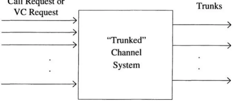
“Trunked Channel” systems
Figure 2 shows a “trunked channel” system. Connection requests (i.e.‚ call setup requests or virtual channel requests) come to the system for a resource‚ i.e.‚ communications channel to be assigned to the request. “Trunks” are shared by multiple users. Each trunk is occupied during the duration of a connection and is reassigned to another connection request when the current call is finished (“loop”).
Figure 2 A general model of a trunked channel system
Offered traffic load
The amount of traffic load offered to a trunked channel system is given by the following equations:
where
– Traffic load generated by a single user; – Total offered traffic load;
– Arrival rate of connection requests per user (i.e.‚ number of connection requests placed by a user per unit time);
– Average call duration per call‚ i.e.‚ “call holding time”; – Number of users served by the system.
Units of traffic load
,
where
– number of busy seconds in one hour;
– “Hundred Call Second;” number of busy seconds during a one-hour period divided by 100;
– amount of traffic load that makes one trunk circuit busy for one hour.
How many is equal to?
By definition‚ is the amount of traffic load that makes one trunk circuit busy for 1 . Since there are in ‚
.
Trunk utilization factor
From the definition of utilization factor‚ the utilization factor of a trunked channel system‚ or trunk utilization factor‚ can be expressed as follows:
,
where – offered load in and – number of trunks. The following statistics provide typical busy-hour statistics:
Loops
Residential ( ‚ i.e.‚ of time);
Business ;
Average ;
Erlang B
The Erlang B system is based on the following assumptions:
Call arrivals‚ i.e.‚ the random arrivals at the trunked channel system‚ are assumed to be Poisson. This implies that the reservoir of arrivals is infinite‚ i.e.‚ the number of end-users generating traffic is infinite. The Erlang B formula provides a conservative estimate of probability of blocking because in reality the number of users is finite.
Call holding times are exponentially distributed.
There are a finite number of channels available in the trunking pool.
“Blocked calls cleared” system. If no channel is available (i.e.‚ “all trunks are busy”) at the time of connection setup request‚ the connection attempt is blocked and cleared from the system‚ i.e.‚ there is no queue for the blocked calls. Hence‚ the Erlang B system may be thought of as a queuing system with zero buffer length.
The QoS measure used for the Erlang B system is the blocking probability: a call or connection request either gets accepted or blocked. The blocking probability‚ , of the Erlang B system is a function of two variables – the offered traffic load in ‚ ‚ and the number of trunks‚ – and is given by the following equation:
.
The above equation is tabulated in the Erlang B Table in terms of the following three parameters:
Blocking probability ( );
Number of channels ( );
Offered load in erlangs ( ).
Given two of the three parameters‚ the value of the third parameter can be found from the Erlang B table‚ i.e.‚
Given and ‚ can be found. Given and ‚ can be found. Given and ‚ can be found.
For given problem we have:
.
Erlang C Mean Delay
Erlang C system
The same assumptions as those for the Erlang B system apply to the Erlang C system except that‚ in the Erlang C system‚ the blocked calls are queued instead of being cleared. The Erlang C system is called the “Blocked Calls Delayed” system. An example of the Erlang C system is the call attendant service‚ where a blocked call is put in a queue with a recorded message playing in the background‚ “your call is important to us ...” The initial blocking probability is given by the following equation‚ which is tabulated in mathematical tables:
.
In the Erlang C system‚ there is only delay and no blocking. The probability that delay will exceed a value is given by the following equation‚ which is the product of the initial blocking probability of previous equation and the second term of the exponential function:
, where
– total offered load in ; – number of trunked channels; – time in ;
– average holding time in .
The mean delay is given by the following equation: