Characterization from Noisy Web Data
Tamara L. Berg1, Alexander C. Berg2, and Jonathan Shih3
1
Stony Brook University, Stony Brook NY 11794, USA,
2
Columbia University, New York NY 10027, USA,
3
University of California, Berkeley, Berkeley CA 94720, USA,
Abstract. It is common to use domain specific terminology – attributes – to describe the visual appearance of objects. In order to scale the use of these describable visual attributes to a large number of categories, espe-cially those not well studied by psychologists or linguists, it will be neces-sary to find alternative techniques for identifying attribute vocabularies and for learning to recognize attributes without hand labeled training data. We demonstrate that it is possible to accomplish both these tasks automatically by mining text and image data sampled from the Internet. The proposed approach also characterizes attributes according to their visual representation: global or local, and type: color, texture, or shape. This work focuses on discovering attributes and their visual appearance, and is as agnostic as possible about the textual description.
1
Introduction
Recognizing attributes of objects in images can improve object recognition and classification as well as provide useful information for organizing collections of images. As an example, recent work on face recognition has shown that the output of classifiers trained to recognize attributes of faces – gender, race, etc. – can improve face verification and search [1, 2]. Other work has demonstrated recognition of unseen categories of objects from their description in terms of attributes, even withno training images of the new categories [3, 4] – although labeled training data is used to learn the attribute appearances. In all of this previous work, the sets of attributes used are either constructedad hocor taken from an application appropriate ontology. In order to scale the use of attributes to a large number of categories, especially those not well studied by psychologists or linguists, it will be necessary to find alternative techniques for identifying attribute vocabularies and for learning to recognize these attributes without hand labeled data.
This paper explores automatic discovery of attribute vocabularies and learn-ing visual representations from unlabeled image and text data on the web. For example, our system makes it possible to start with a large number of images
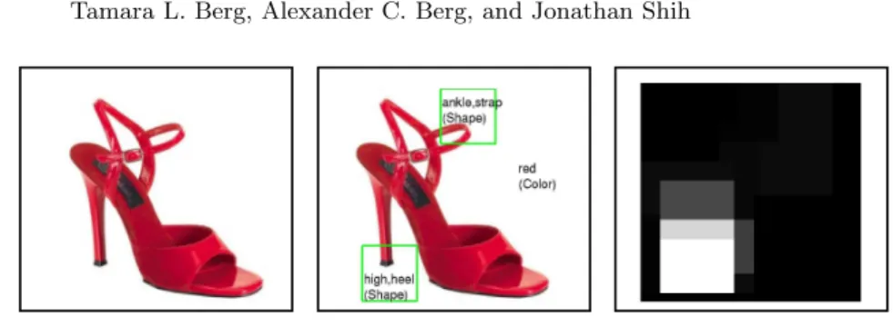
Fig. 1.Original input image (left), Predicted attribute classification (center), and Prob-ability map for localization of “high,heel” (right – white indicates high probProb-ability).
of shoes and their text descriptions from shopping websites and automatically learn that “stiletto” is a visual attribute of shoes that refers to the shape of a specific region of the shoe (see Fig 6). This particular example illustrates a potential difficulty of using a purely language based approach to this problem. The word “stiletto” is a noun that refers to a knife, except, of course, in the context of women’s shoes. There are many other examples, “hobo” can be a homeless person or a type of handbag (purse), “wedding” can be a visually dis-tinctive (color!) feature of shoes, “clutch” is a verb, but also refers to a type of handbag. Such domain specific terminology is common and poses difficulties for identifying attribute vocabularies using a generic language based approach. We demonstrate that it is possible to make significant progress by analyzing the connection between text and images using almost no language specific analysis, with the understanding that a system exploiting language analysis in addition to our visual analysis would be a desireable future goal.
Our approach begins with a collection of images with associated text and ranks substrings of text by how well their occurence can be predicted from visual features. This is different in several respects from the large body of work on the related problem of automatically building models for object category recognition [5, 6]. There, training images are labeled with the presence of an object, with the precise localization of the object or its parts left unknown. Two important differences are that, in that line of work, images are labeled with the name of an object category by hand. For our experiments on data from shopping websites, images are not hand curated for computer vision. For example, we do know the images of handbags in fact contain handbags with no background clutter, but the text to image relationship is significantly less controlled than the label to image relationship in other work – e.g., it is quite likely that an image showing a black shoe will not contain the word “black” in its description. Furthermore there are a range of different text terms that refer to the same visual attribute (e.g., “ankle strap” and “strappy”). Finally, much of the text associated with the images does not in fact describe any visual aspect of the
object (see Fig. 2). We must identify the wheat from amidst a great deal of chaff.
More related to our work are a series of papers modeling the connection between words and pictures [7–10]. These address learning the relationships be-tween text and images at a range of levels – including learning text labels asso-ciated with specific regions of images. Our focus is somewhat different, learning vocabularies of attributes for particular object categories, as well as models for the visual depiction of these attributes. This is done starting with more free-form text data than that in corel [7] or art catalogues [8]. We use discriminative instead of generative machine learning techniques. Also this work introduces the goal of ranking attributes by visualness as well as exploring ideas of attribute characterization.
The process by which we identify which text terms are visually recognizable tells us what type of appearance features were used to recognize the attribute – shape, color, or texture. Furthermore, in order to determine if attributes are localized on objects, we train classifiers based on local sets of features. As a result, we can not only rank attributes by how visually recognizable they are, but also determine whether they are based on shape, color, or texture features, and whether they are localized – referring to a specific part of an object, or global – referring to the entire object.
Our contributions are:
1. Automatic discovery (and ranking) of visual attributes for specific types of objects.
2. Automatic learning of appearance models for attributes without any hand labeled data.
3. Automatic characterization of attributes on two axes: the relevant appear-ance features – shape, color, or texture – and the localizability – localizable or global.
Approach:
Our approach starts with collecting images and associated text descriptions from the web (Sec 4.1). A set of strings from the text are considered as possible at-tributes and ranked by visualness (Sec 2). Highly ranked atat-tributes are then characterized by feature type and localizability (Sec 3.1). Performance is evalu-ated qualitatively, quantitatively, and using human evaluations (Sec 4).
1.1 Related Work
Our key contribution is automatic discovery of visual attributes and the text strings that identify them. There has been related work on using hand labeled training data to learn models for a predetermined list (either formed by hand or produced from an available application specific ontology) of attributes [2–4, 1]. Recent work moves toward automating part of the attribute learning process, but is focused on the constrained setting of butterfly field guides and uses hand coded visual features specific to that setting, language templates, and predefined attribute lists (lists of color terms etc) [11] to obtain visual representations from
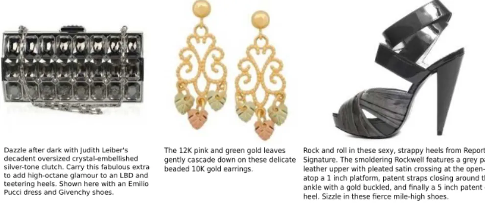
Fig. 2.Example input data (images and associated textual descriptions). Notice that the textual descriptions are general web text, unconstrained and quite noisy, but often provide nice visual descriptions of the associated product.
text alone. Our goal is instead to automatically identify an attribute vocabu-lary and visual representations for these attributes without the use of any prior knowledge.
Our discovery process identifies text phrases that can be consistently pre-dicted from some aspect of visual appearance. Work from Barnard et al,e.g.[9], has looked at estimating the visualness of text terms by examining the results of web image search using those terms. Ferrari and Zisserman learn visual models of given attributes (striped, red, etc) using web image search for those terms as training data [12]. Other work has automatically associated tags for photographs (in Corel) with segments of images [7]. Our work focuses on identifying an at-tribute vocabulary used to describe specific object categories (instead of more general images driven by text based web search for a given set of terms) and characterizes attributes by relevant feature types and localizability.
As mentioned before, approaches for learning models of attributes can be similar to approaches for learning models of objects. These include the very well known work on the constellation model [5, 6], where images were labeled with the presence of an object, but the precise localization of the object and its parts were unknown. Variations of this type of weakly supervised training data range from small amounts of uncertainty in precise part locations when learning pedestrian detectors from bounding boxes around whole a figure [13] to large amounts of uncertainty for the location of an object in an image[14, 5, 6, 15]. At an extreme, some work looks at automatically identifying object categories from large numbers of images showing those categories with no per image labels [16, 17], but even here, the set of images is chosen for the task. Our experiments are also close work on automatic dataset construction [18– 22], that exploits the connection between text and images to collect datasets, cleaning up the noisy “labeling” of images by their associated text. We start
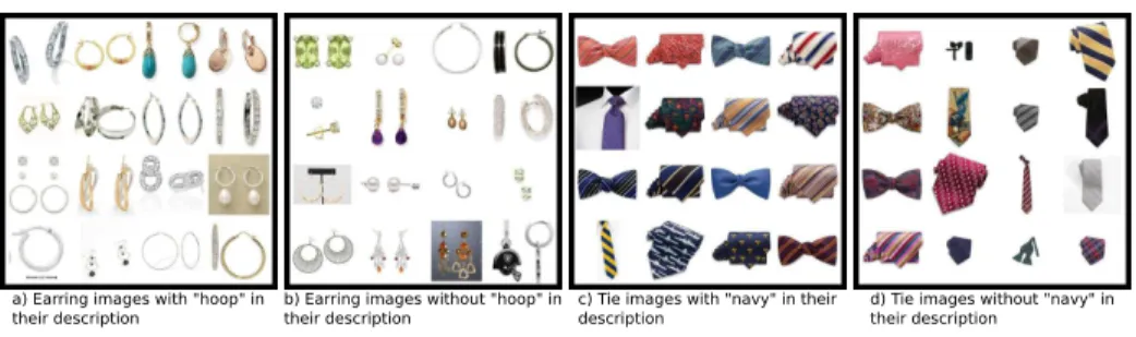
Fig. 3.Example input images for 2 potential attribute phrases (“hoops”, and “navy”). On the left of each pair (a,c) we show randomly sampled images that have the attribute word in their description. On the right of each pair (b,d) we show randomly sampled images that do not have the attribute word in their description. Note that these la-bels are very noisy – images that show “hoops” may not contain the phrase in their description, images described as “navy” may not depict navy ties.
with data for particular categories, rank attributes by visualness, and then go into a more detailed learning process to identify the appropriate feature type and localizability of attributes using the multiple instance learning and boosting (MILboost) framework introduced by Viola [23].
2
Predicting Visualness
We start by considering a large number of strings (Sec. 4) as potential attributes – for instance any string that occurs frequently in the data set can be considered. A visual classifier is trained to recognize images whose associated text contains the potential attribute. The potential attributes are then ranked by their average precision on held out data.
For training a classifier for potential attribute with text representationX, we use as positive examples those images whereX appears in its description, and randomly sample negative examples from those images whereXdoes not appear in the description. There is a fair amount of noise in this labeling (described in Section 4, see fig 3 for examples), but overall for good visual attribute strings there is a reasonable signal for learning. Because of the presence of noise in the labels and the possibility of overfitting, we evaluate accuracy on a held out validation set – again, all of the “labels” come directly from the associated, noisy, web text with no hand intervention.
We then rank the potential attributes by visualness using the learned clas-sifiers by measuring average labeling precision on the validation data. Because boosting has been shown to produce accurate classifiers with good generalization, and because a modification of this method will be useful later for our localizabil-ity measure, we use AnyBoost on decision stumps as our classification scheme. Whole image based features are used as input to boosting (sec 4.2 describes the low level visual feature representations).
2.1 Finding Visual Synsets
The web data for an object category is created on and collected from a vari-ety of internet sources (websites with different authors). Therefore, there may be several attribute phrases that describe a single visual attribute. For exam-ple, “Peep-Toe” and “Open-Toe” might be used by different sources to describe the same visual appearance characteristic of a shoe. Each of these attribute phrases may (correctly) be identified as a good visual attribute, but their re-sulting attribute classifiers might have very similar behavior when applied to images. Therefore, using both as attributes would be redundant.
Ideally, we would like to find a comprehensive, but also compact collection of visual attributes for describing and classifying an object class. To do so we use estimates of Mutual Information to measure the information provided by a collection of attributes to determine whether a new attribute provides signifi-cantly different information than the current collection, or is redundant and can therefore might be considered a synonym for one of the attributes already in the collection. We refer to a set of redundant attributes providing the same visual information as avisual synsetof cognitive visual synonyms. To build a collection of attributes, we iteratively consider adding attributes to the collection in order by visualness. They are added provided that they provide significantly more mu-tual information for their text labels than any of the attributes already in the set. Otherwise we assign the attribute to the synset of the attribute currently in the collection that provided the most mutual information. This process results in a collection of attribute synsets that cover the data well, but tend not to be visually repetitive.
Example Shoe Synsets
{“sandal style round”, “sandal style round open”, “dress sandal”, “metallic”} {“stiletto”, “stiletto heel”, “sexy”, “traction”, “fabulous”, “styling”} {“running shoes”, “synthetic mesh”, “mesh”, “stability”, “nubuck”, “molded”...}
{“wedding”, “matching”, “satin”, “cute”}
Example Handbag Synsets
{“hobo”, “handbags”, “top,zip,closure”, “shoulder,bag”, “hobo,bag”} {“tote”, “handles”, “straps”, “lined”, “open”...}
{“mesh”, “interior”, “metal”} {“silver”, “metallic”}
Alternatively, one could try to merge attribute strings based on text analysis – for example merging attributes with high co-occurence or matching substrings. However, co-occurence would be insufficient to merge all ways of describing a visual attribute,e.g., “peep-toe” and “open-toe” are two alternative descriptions for the same visual attribute, but would rarely be observed in the same textual description. Matching substrings can lead to incorrect merges, e.g., “peep-toe” and “closed-toe” share a substring, but have opposing meanings. Our method for visual attribute merging based on mutual information overcomes these issues.
3
Attribute Characterization
For those attributes predicted to be visual, we would like to make some fur-ther characterizations. To this end, we present methods to determine whefur-ther an attribute is localizable (Section 3.1) – ie does the attribute refer to a global
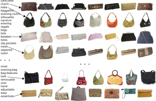
Fig. 4.Automatically discovered handbag attributes, sorted by visualness.
appearance characteristic of the object or a more localized appearance charac-teristic? We also provide a way to identify attribute type (Section 3.2) – ie is the attribute indicated by a characteristic shape, color, or texture?
3.1 Predicting Localizability
In order to determine whether an attribute is localizable – whether it usually corresponds to a particular part on an object, we use a technique based on MILBoost [23, 14] on local image regions of input images. If regions with high probability under the learned model are tightly clustered in the training images we consider the attribute localizable. Figure 1 shows an example of the predicted probability map on an image for the “high heel” attribute and our automatic attribute labeling.
MILBoost is a multiple instance learning technique using AnyBoost, first introduced in Viola et al [23] for training face detectors, and later used for other object categories [14]. MILBoost builds a classifier by incrementally selecting a set of weak classifiers to maximize classification performance, re-weighting the training samples for each round of training. In the end each bag receives a probability under the model, as does each sample. Because the text descriptions do not specify what portion of image is described by the attribute, we have a multiple instance learning problem where each image (data item) is treated as a bag of regions (samples) and a label is associated with each image rather than each region.
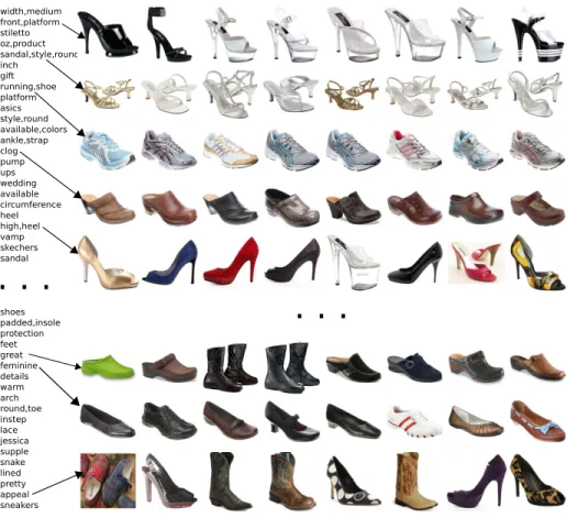
Fig. 5.Automatically discovered shoe attributes, sorted by visualness.
If iindexes images, and j indexes segments and the boosted classifier pre-dicts the score of a sample as a linear combination of weak classifiers: yij =
P
tλtct(xij). Then the probability that segment j in imagesi is a positive ex-ample is
pij =
1
1 +exp(−yij) (1)
The probability of an image being positive is then (under the noisy OR model), one minus the probability of all segments being negative.
pi= 1−
Y
j∈i
(1−pij) (2)
Following the AnyBoost technique, the weight,wij assigned to each segment is the derivative of the cost function with respect to a change in the score of the segment (whereti is the label of imagei∈0,1):
wij =
ti−pi
pi
Each round of boosting selects the weak classifier that maximizes:Pijc(xijwij), where c(xij) is the score assigned to the segment by the weak classifier and
c(xij) ∈ −1,+1. The weak classifier weight parameter, λt is determined using line search to maximize the log-likelihood of the new combined classifier at each iterationt.
Localizabilityof each attribute is then computed by evaluating the trained MILBoost classifier on a collection of images associated with the attribute. If the classifier tends to give high probability to a few specific regions on the object (i.e., only a small number of regions have largePij), then the attribute is localizable. If the probability predicted by the model tends to be spread across the whole object then the attribute is a global characteristic of the object. To measure the attribute spread, we accumulate the predicted attribute probabilities over many images of the object and measure the localizability as the portion of image needed to capture the bulk of this accumulated probability (the portion of all
Pij’s containing at least 95% of the predicted probability). If this is a small percentage of the image then we predict the attribute as localizable. For our current system, we have focused on product images which tend to be depicted from a relatively small set of possible viewpoints (shoe pointed left, two shoes etc). This means that we can reliably measure localization on a rough fixed grid across the images. For more general depictions, an initial step of alignment or pose clustering [24] could be used before computing the localizability measure.
3.2 Predicting Attribute Type
Our second attribute characterization classifies each visual attribute as one of 3 types: color attributes, texture attributes and shape attributes. Previous work has concentrated mostly on building models to recognize color (e.g., “blue”) and texture (e.g., “spotty”) based attributes. We also consider shape based at-tributes. These shape based attributes can either be indicators of global object shape (e.g., “shoulder bag”) or indicators of local object shape (e.g., “ankle strap”) depending on whether they refer to an entire object or a part of an object. For each potential attribute we train a MILBoost classifier on three dif-ferent feature types (color, texture, or shape – visual representation described in Section 4.2). The best performing feature measured by average precision is selected as the type.
4
Experimental Evaluation
We have performed experiments evaluating all aspects of our method: predicting visualness (Section 4.3), predicting the localizability (Section 4.4), and predicting type (Section 4.4). First we begin with a description of the data (Section 4.1), and the visual and textual representations (Section 4.2).
4.1 Data
We have collected a large data set of product images from the internet4
depict-ing four broad types of objects: shoes, handbags, earrdepict-ings, and ties. In total we 4
specifically from like.com, a shopping website that aggregates product data from a wide range of e-commerce sources
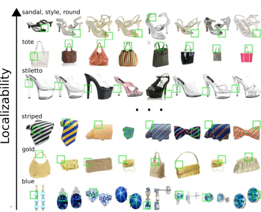
Fig. 6.Attributes sorted by localizability. Green boxes show most probable region for an attribute.
have 37795 images: 9145 images of handbags, 14765 images of shoes, 9235 im-ages of earrings, and 4650 imim-ages of ties. Though these imim-ages were collected from a single website aggregator, they originate from a variety of over 150 web sources (e.g., shoemall, zappos, shopbop), giving us a broad sampling of various categories for each object type both visually and textually (e.g., the shoe images depict categories from flats, to heels, to clogs, to boots). These images tend to be relatively clean, allowing us to focus on the attribute discovery goal at hand without confounding visual challenges like clutter, occlusion etc.
On the text side however the situation is extremely noisy. Because this general web data, we have no guarantees that there will be a clear relationship between the images and associated textual description. First there will be a great number of associated words that are not related to visual properties (see fig 2). Secondly, images associated with an attribute phrase might not depict the attribute at all, also, and quite commonly, images of objects exhibiting an attribute might not contain the attribute phrase in their description (see fig 3). As the images originate from a variety of sources, the words used to describe the same visual attribute may vary. All these effects together produce a great deal of noise in the labelingthat can confound the training of a visual classifier.
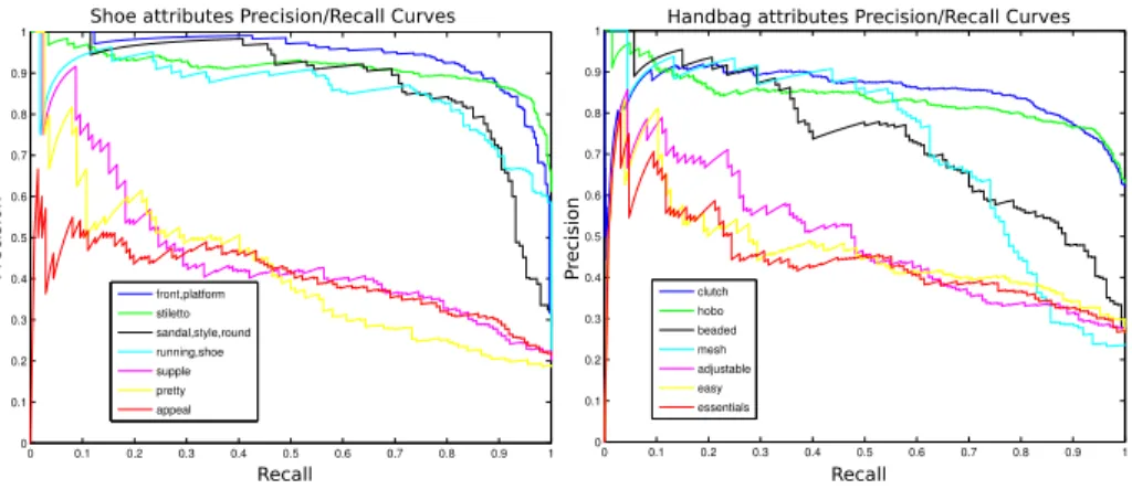
Fig. 7. Quantitative Evaluation: Precision/Recall curves for some highly visual at-tributes, and other less visual attributes for shoes (left) and handbags (right).
4.2 Representations
Visual Representation:We use three visual feature types: color, texture, and shape. For predicting the visualness of a proposed attribute we take a global descriptor approach and compute whole image descriptors for input to the Any-Boost framework. For predicting localizability and attribute type, we take a local descriptor approach, computing descriptors over local subwindows in the image with overlapping blocks sampled over the image (with block size 70x70 pixels, sampled every 25 pixels).
Each of our three feature types is encoded as a histogram (integrated over the whole image for global descriptors, or over individual regions for local de-scriptors), making selection and computation of decision stumps for our boosted classifiers easy and efficient. For the shape descriptor we utilize a SIFT visual word histogram. This is computed by first clustering a large set of SIFT descrip-tors using k-means (withk= 100) to get a set of visual words. For each image, the SIFT descriptors are computed on a fixed grid across the image, then the resulting visual word histograms are computed. For our color descriptor we use a histogram computed in HSV with 5 bins for each dimension. Finally, for the texture descriptor we first convolve the image with a set of 16 oriented bar and spot filters [25], then accumulate absolute response to each of the filters in a texture histogram.
Textual Representation:On the text side we keep our representation very simple. After converting to lower case, removing stop words, and punctuation, we consider all remaining strings of up to 4 consecutive words that occur more than 200 times as potential attributes.
4.3 Evaluating Visualness Ranking
Some attribute synsets are shown for shoes in figure 5 and for handbags in fig-ure 4, where each row shows some highly ranked images for an attribute synset.
Fig. 8.Attributes from the top and bottom of our visualness ranking for earrings as compared to a human user based attribute classification. The user based attribute classification produces similar results to our automatic method (80% agreement for earrings, 70% for shoes, 80% for handbags, and 90% for ties).
For shoes, the top 5 rows show highly ranked visual attributes from our collec-tion: “front platform”, “sandal style round”, “running shoe”, “clogs”, and “high heel”. The bottom 3 rows show less highly ranked visual attributes: “great”, “feminine”, and “appeal”. Note that the predicted visualness seems reasonable. This is evaluated quantitatively below. For handbags, attributes estimated to be highly visual include terms like “clutch”, “hobo”, “beaded”, “mesh” etc. Terms estimated by our system to be less visual include terms like “look”, “easy”, “adjustable” etc.
The visualness ranking is based on aquantitative evaluationof the classi-fiers for each putative attribute. Precision recall curves on our evaluation set for some attributes are shown in figure 7 (shoe attributes left, handbag attributes right). Precision and recall are measured according to how well we can predict the presence or absence of each attribute term in the images textual descrip-tions. This measure probes both the underlying visual coherence of an attribute term, and whether people tend to use the term to describe objects displaying the visual attribute. For many reasonable visual attributes our boosted classifier performs quite well, getting average precision values of 95% for “front platform”, 91% for stiletto, 88% for “sandal style round”, 86% for “running shoe” etc. For attributes that are probably less visual the average precision drops to 46% for “supple”, 41% for “pretty”, and 40% for “appeal”. This measure allows us to reasonably predict the visualness of potential attributes.
Lastly we obtain a human evaluationof visualness and compare the re-sults to those produced by our automatic approach. For each broad category types, we evaluate the top 10 ranked visual attributes (classified as visual by our
algorithm), and the bottom 10 ranked visual attributes (classified as non-visual by our algorithm). For each of these proposed attributes we show 10 labelers (using Amazon’s Mechanical Turk) a training set of randomly sampled images with that attribute term and without the term. They are then asked to label novel query images, and we rank the attributes according to how well their labels predict the presence or absence of the query term in the corresponding descrip-tions. The top half of this ranking is considered visual, and the bottom half as non-visual (seee.g., fig 8). Classification agreement between the human method and our method is: 70% for shoes, 80% for earrings, 80% for bags, and 90% for ties, demonstrating that our method agrees well with human judgments of attribute visualness.
4.4 Evaluating Characterization
Localizability:Some examples of highly localizable attributes are shown in the top 4 rows of figure 6. These include attributes like “tote”, where MILBoost has selected the handle region of each bag as the visual representation, and “stiletto” which selects regions on the heel of the shoe. For “sandal style round” the open toe of the sandal is selected as the best indicator for this attribute. And, for “asics” the localization focuses on the logo region of the shoe which is present in most shoes of the asics brand. Some examples of more global attributes are shown in the bottom 2 rows of figure 6. As one might expect, some less localizable attributes are based on color (e.g., “blue”, “red” etc) and texture (e.g., “paisley”, “striped”).
Type: Attribute type categorization works quite well for color attributes, predicting “gold”, “white”, “black”, “silver” etc as colors reliably in each of our 4 broad object types. One surprising and interesting find is that “wedding” is labeled as a color attribute. The reason this occurs is that many wedding shoes use a similar color scheme that is learned as a good predictor by the classifier. Our method for predicting type also works quite well for shape based attributes, predicting “ankle strap”, “high heel”, “chandelier”, “heart”, etc to be shape at-tributes. Texture characterization produces more mixed results, characterizing attributes like “striped”, and “plaid” as texture attributes, but other attributes like “suede” or “snake” as SIFT attributes ( perhaps an understandable confu-sion since both feature types are based on distributions of oriented edges).
5
Conclusions & Future Work
We have presented a method to automatically discover common attribute terms. This method is able to reliably find and rank potential attribute phrases accord-ing to their visualness – a score related to how strongly a straccord-ing is correlated with some aspect of an object’s visual appearance. We are further able to char-acterize attributes as localizable (referring to the appearance of some consistent subregion on the object) or global (referring to a global appearance aspect of the object). We also categorize attributes by type (color, texture, or shape). Future work includes improving the natural language side of the system to complement the visually dominated ideas presented here.
References
1. Kumar, N., Berg, A.C., Belhumeur, P., Nayar, S.K.: Attribute and simile classifiers for face verification. In: ICCV. (2009)
2. Kumar, N., Belhumeur, P., Nayar, S.K.: FaceTracer: A search engine for large collections of images with faces. In: ECCV. (2008)
3. Lampert, C., Nickisch, H., Harmeling, S.: Learning to detect unseen object classes by between-class attribute transfer. In: CVPR. (2009)
4. Farhadi, A., Endres, I., Hoiem, D., Forsyth, D.A.: Describing objects by their attributes. In: CVPR. (2009)
5. Fergus, R., Perona, P., Zisserman, A.: Object class recognition by unsupervised scale-invariant learning. In: CVPR. (2003)
6. Fei-Fei, L., Fergus, R., Perona, P.: A Bayesian approach to unsupervised one-shot learning of object categories. In: ICCV. (2003)
7. Duygulu, P., Barnard, K., de Freitas, N., Forsyth, D.: Object recognition as ma-chine translation: Learning a lexicon for a fixed image vocabulary. In: ECCV. (2002)
8. Barnard, K., Duygulu, P., Forsyth, D.: Clustering art. In: CVPR. (2005)
9. Yanai, K., Barnard, K.: Image region entropy: A measure of ’visualness’ of web images associated with one concept. In: WWW. (2005)
10. Barnard, K., Duygulu, P., de Freitas, N., Forsyth, D., Blei, D., Jordan, M.I.: Match-ing words and pictures. JMLR3(2003) 1107–1135
11. Wang, J., Markert, K., Everingham, M.: Learning models for object recognition from natural language descriptions. In: BMVC. (2009)
12. Ferrari, V., Zisserman, A.: Learning visual attributes. NIPS (2007)
13. Felzenszwalb, P.F., Girshick, R.B., McAllester, D., Ramanan, D.: Object detection with discriminatively trained part based models. PAMI99(2009)
14. Galleguillos, C., Babenko, B., Rabinovich, A., Belongie, S.: Weakly supervised object recognition and localization with stable segmentations. In: ECCV. (2008) 15. Everingham, M., Zisserman, A., Williams, C., L. Van Gool e.a.: Pascal voc
work-shops (2005-2009)
16. Sivic, J., Russell, B.C., Efros, A.A., Zisserman, A., Freeman, W.T.: Discovering objects and their location in images. In: ICCV. (2005)
17. Sivic, J., Russell, B.C., Zisserman, A., Freeman, W.T., Efros, A.A.: Discovering object categories in image collections. In: ICCV. (2005)
18. Berg, T.L., Forsyth, D.: Animals on the web. In: CVPR. (2006)
19. Schroff, F., Criminisi, A., Zisserman, A.: Harvesting image databases from the web. In: ICCV. (2007)
20. Berg, T.L., Berg, A.C.: Finding iconic images. In: CVPR Internet Vision Work-shop. (2009)
21. Berg, T.L., Berg, A.C., Edwards, J., Forsyth, D.A.: Who’s in the picture. NIPS (2004)
22. Collins, B., Deng, J., Li, K., Fei-Fei, L.: Towards scalable dataset construction: An active learning approach. In: ECCV. (2008)
23. Viola, P., Plattand, J., Zhang, C.: Multiple instance boosting for object detection. In: NIPS. (2007)
24. Berg, A.C., Berg, T.L., Malik, J.: Shape matching and object recognition using low distortion correspondence. In: CVPR. (2005)
25. Leung, T., Malik, J.: Representing and recognizing the visual appearance of ma-terials using three-dimensional textons. IJCV43(2001) 29–44