Vol 5, No 02 (2017)

V.B. Kumar Vatti et al IJSRE Volume 05 Issue 02 February 2017 Page 6212

Volume||5||Issue||02||February-2017||Pages-6212-6216||ISSN(e):2321-7545 Website: http://ijsae.in

Index Copernicus Value- 56.65 DOI: http://dx.doi.org/10.18535/ijsre/v5i02.04

A Fourth Order Variant of Newton’s Method

Authors

V.B. Kumar Vatti1 , Ramadevi Sri2 , M.S.Kumar Mylapalli3

1

Dept. of Engineering Mathematics, Andhra University, Visakhapatnam, India, 2

Dept. of Engineering Mathematics, Andhra University, Visakhapatnam, India, 3

Dept. of Engineering Mathematics, Gitam University, Visakhapatnam, India, Email- [email protected], [email protected], [email protected] ABSTRACT:

In this paper, we present a new two step iterative method to solve the nonlinear equation f x 0 and

discuss about its convergence. Few numerical examples are considered to show the efficiency of the new method in comparison with the other methods considered in this paper.

Keywords: Nonlinear equation, Iterative method, Newton’s method, Chebyshev’s method, Convergence.

1. INTRODUCTION

Many of the complex problems in Science and Engineering contains the function of nonlinear equation of the form

  0

f x  (1.1) Where f I: R for an open interval I is a scalar function.

Let 1 x

n be the root of the equation (1.1) i.e., f x

 

n1 0 while f

 

xn1 0.

The classical quadratic convergent Newton‟s method [3] for finding the root of “(1.1),” is

 

 

, 0

1

f xn

x x_n n

n   _{f xn}  (1.2)

The third order two step Chebyshev‟s method [4] is

 

 

f xn y_n x_n

f _xn

 



   

  2

, 0

1 ₂

y_n x_n f x_n

x_n y_n n

f _xn

 

   

 _ (1.3)

The third order Newton‟s variant method [7] is

 

 

2 , 0

1 _{1 1 2}

f xn

x x_n n

n _{f xn}

n



 

    

 _{    }

 

(1.4)

where,    

  2 f x_n f x_n n

f _xn

  



   

.

V.B. Kumar Vatti et al IJSRE Volume 05 Issue 02 February 2017 Page 6213

2. A FOURTH ORDER VARIANT OF NEWTON’S METHOD

Following the basic assumption of Abbasbandy and Maheshweri [1], [2] and also others [5], [6] and [8], we consider the second degree Taylor‟s expansion of

 

1

f x

n about xnis

 

 





 





 

2 1

1 1 ₂

x_{n xn}

f x_n f x_n x_n x_n f x_n f x_n

 

 

   

  (2.1)

Where

1

x x_n h n  

 

2

 

 

 

 

 

2

 

1 1 ₂ 1 ₂

f x_n x_n f x_n

f x x x f x_n x f_n x_n f x_n x f_n x_n

n n n

              _{ } _  _     _{ }  _{ }   (2.2) Since, 1 x

n be the root of the equation (1.1) i.e., f x

 

n1 then the equation (2.2) becomes

 

 

 

 

 

 

2 _{2 2 2 2} 2 ₀

1 1

x _n _f x_{n }x_n _ f x_n  x f_n  x_{n  }_ f x_n  x f_n  x_n x_n f x_{n }_ (2.3)

Rewriting _f

 

f

 

yn f

 

xn xn

y_n x_n

  

 

 and

 

 

2_{f yn}

n

f xn

  in “(1.4),” gives the two step Newton‟s variant

method as

 

 

f xn y_n x_n

f _xn   

 

 

   

2 _{, 0}

1

1 1 4

f xn

x_n x_n n

f x_{n f yn} f xn                     _   (2.4)

The simplified form of “(2.4),” can be rewritten as

 

 

1 1 1 4





12

1 2

f xn

x x_{n n}

n _{f xn} _n 

              _

Expanding



1 4 _n



12up to four terms i.e., up to third degree terms of_n, we get the required two step Newton‟s variant method as

 

 

f xn y_n x_n

f _xn   

 

 

 

 

 

 

2

1 2 , 0

1

f x_n f y_n f y_n

x_n x_n n

f x_n f x_n f x_n

 _{ }            _  _ _      (2.5)

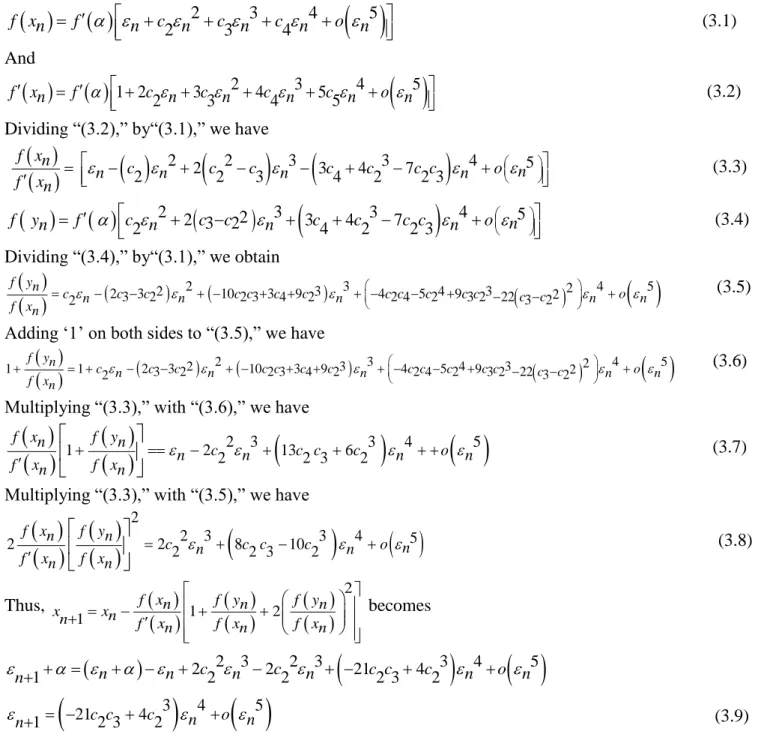
3. CONVERGENCE CRITERIA

Theorem 3.1. Let Ibe a simple zero of a sufficiently differentiable function f I: Rfor an open interval I. Then, the new method that is defined by “(2.5),” has the fourth order convergence and satisfies the following error equation,



_{21 4} 3



4

 

5

1 c c2 3 c2 n o n

n

 _      

Where,

1 1

x

n n  and xn



n



V.B. Kumar Vatti et al IJSRE Volume 05 Issue 02 February 2017 Page 6214

 

 

2 3 4

 

5

2 3 4

f x_n  f  _ _nc _n c _n c _n o _n _

  (3.1)

And

 

 

_{1 2 3} 2 ₄ 3 ₅ 4

 

5 5

2 3 4

f x _n  f  _  c _n c _n  c _n  c _n o _n _ (3.2)

Dividing “(3.2),” by“(3.1),” we have

 

 

 

2 2 2



22 3

 

3 3 4 4 23 7 2 3



4 5

f xn _{c c c c c c c o}

n

n n n n

f _xn     

 

 

 

 

 _        _

 

 (3.3)

 

 

2 ₂



₂



3



_{3 4} 3 ₇



4 5

3 2

2 4 2 2 3

f y_n  f  _c _n  c c _n  c  c  c c _n o__{n }_ (3.4)

Dividing “(3.4),” by“(3.1),” we obtain

 

 

₂



23 322



2



10 2 3 34 9 23



3 4 2 4 524 93 23 _{22 3 2}



2



2 4

 

5 f yn

c _n c c _n c c c c _n c c c c c _{c c n} o _n

f xn     

 

 

 

           _{ }  (3.5)

Adding „1‟ on both sides to “(3.5),” we have

 

 

 2 2  3 3 4 3





2 4

 

5

1 f yn 1 c₂ n 2c3 3c2 n 10c c2 3 3c4 9c2 n 4c c2 4 5c2 9c c3 2 _{22 3 2}c c 2 n o n

f xn     

 

 

 

             _{ }  (3.6)

Multiplying “(3.3),” with “(3.6),” we have

 

 

1

 

 

2 ₂2 3



13 _{2 3} 6 ₂3



4

 

5

f x_n f y_n

c c c c o

n n n n

f x_n  f x_n         

 

 

  (3.7)

Multiplying “(3.3),” with “(3.5),” we have

 

 

 

 





 

2

2 3 3 4 ₅

2 f xn f yn 2c_{2 n} 8c c_{2 3} 10c_{2 n} o _n f x_n f x_n       

 

 

 

(3.8)

Thus,

 

 

 

 

 

 

2

1 2

1

f x_n f y_n f y_n x _xn

n _{f x f x f x}

n n n

 _{ } 

 

     

   _ _ 

 

 

becomes





₂ 2 3 ₂ 2 3



_{21 4} 3



4

 

5

1 n n c2 n c2 n c c2 3 c2 n o n

n

 _               



3



4

 

5

21 4

1 c c2 3 c2 n o n

n

 _      

(3.9)

Equation (3.9) establishes the fourth order convergence of the method that is defined by “(2.5)”.

4. NUMERICAL EXAMPLES

We consider few numerical examples considered by [6], [8] and the method “(2.5),” are compared with the methods “(1.2),” “(1.3),” and “(1.4)”. The computational results are tabulated below and the results are correct up to an error less thanas indicated for each of the problems.

Example 1. Consider the following equation f x

 

ex3x2 0.

Table 4.1.The results obtained by four methods for solving f x

 

ex3x2 0withx₀0.5and 0.5E20.

Formula No. of iterations (n) Root

 

_xn No. of functional values

Newton 7 0.91000757248870907904 14

Chebyshev --- DIVERGENT ---

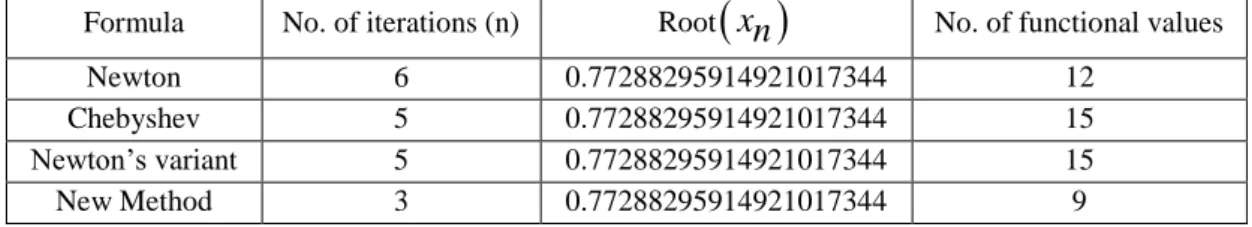
V.B. Kumar Vatti et al IJSRE Volume 05 Issue 02 February 2017 Page 6215 Example 2. Consider the following equation f x

 

x3ex0.

Table 4.2.The results obtained by four methods for solving f x

 

x3ex0withx00.5and 0.5E20.

Example 3. Consider the following equation f x

 

sinx0.5x0.

Table 4.3. The results obtained by four methods for solving f x

 

sinx0.5x0withx₀3and 0.5E20.

Example 4. Consider the following equation f x

 

x32x 5 0.

Table 4.4.The results obtained by four methods for solving f x

 

x32x 5 0withx03and 0.5E20.

Example 5. Consider the following equation f x

 

sinx0.

Table 4.5 The results obtained by four methods for solving f x

 

sinx0withx₀0.5and0.5E20.

5. CONCLUSION

With the number of iterations and the number of functional evaluations tabulated for each of the methods for five non-linear equations, we conclude that the method “(2.5),” is efficient one compared to the methods considered in this paper.

REFERENCES

1. S.Abbasbandy, “Improving Newton-Raphson method for nonlinear equations by modified Adomian decomposition method”, Applied Mathematics and Computation, Vol. 145, 2003, pp. 887 – 893. 2. Amit kumar Maheshwari, “A fourth order iterative method for solving nonlinear equations”, Applied

Mathematics and computation, Vol.211, 2009, pp. 383-391.

3. Avram Sidi, “Unified treatment of regular falsi, Newton–Raphson, Secant, and Steffensen methods for nonlinear equations”, Journal of Online Mathematics and its Applications. 2006, pp. 1-13.

Formula No. of iterations (n) Root

 

xn No. of functional values

Newton 6 0.77288295914921017344 12

Chebyshev 5 0.77288295914921017344 15 Newton‟s variant 5 0.77288295914921017344 15 New Method 3 0.77288295914921017344 9

Formula No. of iterations (n) Root

 

_xn No. of functional values

Newton 6 1.89549426703398109184 12

Chebyshev 5 1.89549426703398109184 15 Newton‟s variant 5 1.89549426703398109184 15 New Method 3 1.89549426703398109184 9

Formula No. of iterations (n) Root

 

_xn No. of functional values Newton 7 2.09455148154232668160 14

Chebyshev 5 2.09455148154232668160 15 Newton‟s variant 5 2.09455148154232668160 15 New Method 3 2.09455148154232668160 9

Formula No. of iterations (n) Root

 

xn No. of functional values

Newton 5 0 10

Chebyshev 4 0 12

Newton‟s variant 4 0 12

V.B. Kumar Vatti et al IJSRE Volume 05 Issue 02 February 2017 Page 6216 4. J.M.Gutierrez, M.A.Hernandez, “A family of Chebyshev-Halley type methods in Banach spaces”,

Bull. Aust. Math. Soc. 55, 113-130 (1997).

5. Jinhai Chen, Weiguo Li, “On new exponential quadratically convergent iterative formulae”, Applied Mathematics and Computation, Vol. 180, 2006, pp. 242-246.

6. Nasr Al-Din Ide, “A new Hybrid iteration method for solving algebraic equations”, Applied Mathematics and Computation, Vol. 195, 2008, pp. 772-774.

7. Vatti V.B.Kumar., Ramadevi Sri., Mylapalli M. S. Kumar., “A Newton‟s Variant third order method”, Engineering Science and Technology: An International Journal, Vol. 6, No. 4, 2016. 8. Xing-Guo Luo, “A note on the new iterative method for solving algebraic equation”, Applied