Abstract
A computationally efficient beam element is presented for the finite element (FE) anal-ysis of framed structures with multiple concentrated damages. The proposed model is able to account for any number and location of cracks, whose macroscopic effects are simulated with a set of longitudinal, rotational and transverse elastic springs at the position of each singularity, which in turn can be mathematically represented with pos-itive (physically consistent) Dirac’s deltas in the corresponding flexibility functions. The commercial finite element (FE) code SAP2000 is used to validate the proposed approach for both static and dynamic loads. Interestingly, a very similar multi-cracked beam (MCB) element has been recently formulated by other researchers, who have in-dependently exploited negative (physically inconsistent) Dirac’s deltas in the stiffness functions to model the concentrated damage, getting however the same discontinuous shape functions for the FE formulation. Although derived and tested within the linear range, the proposed approach lends itself to be easily extended to include a non-linear constitutive law for the concentrated damages.
Keywords: cracked beams, Euler-Bernoulli beam theory, damaged structures, finite element analysis, Timoshenko beam theory.
1
Introduction
Presence of cracks in framed structures may substantially change their static and dy-namic response, reducing the performance and eventually causing the failure. Broadly speaking, the approaches available in the literature to model cracks in beams and columns can be classified into three main categories: local stiffness reduction (LSR), discrete spring (DS) equivalent models, and more sophisticated formulations adopting methods and concepts of Fracture Mechanics [1].
Paper 257
A Two-Node Multi-Cracked Beam Element for
Static and Dynamic Analysis of Planar Frames
M. Donà
1, A. Palmeri
1, A. Cicirello
2and M. Lombardo
11
School of Civil and Building Engineering
Loughborough University, United Kingdom
2
Engineering Department
University of Cambridge, United Kingdom
©Civil-Comp Press, 2012
Proceedings of the Eleventh International Conference on Computational Structures Technology,
B.H.V. Topping, (Editor),
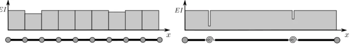
Figure 1: The bending stiffnessEI for the LSR (left) and DS (right) models
The LSR can be considered as the simplest method to build a finite element (FE) model of a damaged beam, as it simply requires to mesh the beam with a sufficient number of beam elements and to reduce the relevant stiffness component (e.g. the flexural stiffness) of the element at the position where the crack occurs (see Figure 1 (left)) [2, 3, 4]. To be efficient, this approach requires a fine mesh, and the problem arises of quantifying the stiffness reduction in each FE to match the global effects of the actual crack.
In the DS model, on the contrary, the damage is lumped at a single point, as the beam is ideally divided at the position of the damage in two regions. The new ele-ments so obtained are articulated at the location of the crack, and the residual stiffness is simulated by axial, rotational and shear springs. For slender beams in bending, however, the presence of cracks affects mainly the flexural stiffnessEI, and therefore the DS model just consists of joining the elements on the two sides of the crack with a hinge (i.e. axial and shear flexibility are not considered), which are then coupled with a rotational spring, whose stiffness is related to the intensity of the damage (see Figure 1 (right)): that is, the severer the damage, the softer is the spring. The main shortcoming with the DS model is that, if a conventional beam element is used, two additional FE nodes must be placed at the location of each crack, i.e. one node on each side of the crack. This could be particularly cumbersome if the DS model is used for the purposes of damage identification, as it would require re-meshing the beam during the identification process.
Alternatively, the use of 2D or 3D FE models may produce very detailed and ac-curate results, but such computationally intensive approaches are more appropriate to tackle problems of crack initiation and/or propagation, while global analysis of framed structures and crack detection in beams and columns can be carried out by less sophis-ticated FE models. As a matter of fact, the DS model often provides the best trade-off between accuracy and computational effort for these applications.
Motivated by these considerations, many formulations have been developed for the DS model, including the “rigidity modelling” by Biondi and Caddemi [5, 6], in which the singularities in the flexural stiffness, corresponding to concentrated damages, are introduced as negative impulses (i.e. Dirac’s delta functions with negative sign). Al-though expedient, this mathematical representation is not consistent with the definite-positive nature of the flexural stiffness, delivering however exact closed-form solutions for the static analysis of multi-cracked slender beams in bending. Aimed at overcom-ing this intrinsic theoretical flaw, Palmeri and Cicirello [7] have recently presented a (physically consistent) dual representation of cracks, i.e. a “flexibility modelling”, in which Dirac’s delta functions with positive sign are introduced in the bending
flexibil-ity of the beam, i.e. the inverse of its flexural stiffness; they also extended the model to cope with Timoshenko beams, to take into account the contribution of the shear deformations in the uncracked regions of the member.
A further distinction in the formulations available in the technical literature for the DS model can be made between “always open” and “breathing” cracks [1, 8, 9, 10]. The first representation is mainly used for static problems, but it can be adopted for dynamic loadings as well, provided that the static deflection in the damaged members is larger than the vibration amplitude. This model is particularly useful for frames behaving elastically and experiencing small displacements, as the structural response of the damaged system remains linear. If the crack opens and closes as the direction of the dynamic input reverses, a bi-linear breathing model is more appropriate, leading to complicated non-linear phenomena (e.g. [11, 12]). Both representations have been ex-tensively studied and applied within different schemes of structural health monitoring, aimed at identifying presence, location and severity of concentrated damage in framed structures (e.g. References [13] to [18]. In this context, the size of the finite element (FE) model for the structural frame under investigation plays an important role, as ideally it should be as small as possible. Indeed, the vast majority of the identification algorithms proceed iteratively until convergence, and therefore any little saving in the computational cost for a single analysis may result in a significant advantage on the whole process. Moreover, as already pointed out above, traditional damage detection approaches may require FE re-meshing throughout the identification process, which inevitably causes an additional increase in the computational effort.
Aimed at addressing these issues, an analytical and numerical study has been car-ried out to develop an efficient two-node multi-cracked beam (MCB) element for the FE analysis of framed structures with concentrated damages, whose key feature is the capacity to account for any number and location of cracks without increasing the size of the problem in comparison with the corresponding undamaged structure.
It is worth mentioning here that similar approaches have been recently pursued by other authors, whose studies differ in the analytical formulations adopted to get the closed-form expressions for stiffness matrix, load vector and mass matrix. In the MCB element proposed by Skrinar [19], cubic splines are used to represent the field of transverse displacements in each uncracked region of the beam, while the additional kinematic and static unknowns arising at each crack have been eliminated with the help of compatibility and equilibrium equations combined with the Hooke’s law for the rotational springs simulating the cracks. However, this study has only considered slender Euler-Bernoulli beams in bending and masses lumped at the two nodes of the resulting MCB element, which may limit its applicability.
The formulation proposed by Caddemi et al. [20] is more comprehensive, as it includes the shear deformations (i.e. the Timoshenko beam theory has been adopted), and rotational and transverse springs are considered at the position of each crack. They have employed the (physically inconsistent) “rigidity modelling” of concentrated damage to derive the exact closed-form expressions for the deformed shape of the two-node MCB element subjected to unitary nodal settlements, which in turn have been
used to derive the stiffness matrix and consistent mass matrix.
In this paper, a very similar approach, independently pursued by the authors us-ing the dual representation of cracks proposed by Palmeri and Cicirello [7], will be presented and numerically validated. The main differences in comparison with the formulation developed by Caddemi et al. [20] are: i) the axial damage is included in the MCB element, so that it is possible to consider for each crack a set of axial, rota-tional and shear springs, i.e. the beam is fully articulated at the position of the cracks, allowing relative longitudinal, rotational and transverse movements; ii) the (physi-cally consistent) “flexibility modelling” of concentrated damage is resorted to; and iii) our analyses are limited to planar frames, while 3D frames have been considered by Caddemi et al. [20].
The paper aims to demonstrate the improved efficiency of the two-node MCB el-ement with respect to the LSR model. To do this, the results of static analyses are validated against those provided by the commercial FE code SAP2000. It is shown that, independently of the number of cracks, the proposed MCB element is able to deliver, for both Euler-Bernoulli and Timoshenko kinematic models, the same exact solutions with just a single FE for each beam and column in the framed structure, while the LSR model only gives an approximate solution (whose accuracy depends on the size of the mesh) and SAP2000 needs an additional node at the position of each crack. Both lumped and consistent mass matrices have been also tested for the modal analyses. It is shown that using lumped masses with the proposed MCB element al-lows recovering the same eigenproperties given by SAP2000, provided that the same mesh is adopted, i.e. with two FE nodes at each crack location; while using the consis-tent mass matrix increases the accuracy, as the eigenproperties so obtained converge more rapidly to the exact solution, with the additional advantage that the FE mesh is totally independent of the position of the cracks.
2
Exact closed-form solutions for beams with multiple
cracks under axial and transverse loads
Aimed at defining the shape functions for the proposed MCB element, the flexibility modelling recently proposed by Palmeri and Cicirello [7] for a concentrated flexural damage (i.e. a crack-induced lumped rotation) has been extended to include axial and shear lumped deformations at the position of the crack, and has been then used to de-rive the exact closed-form solutions for multi-cracked beams subjected to both axial and transverse loads. For the sake of brevity, the mathematical derivation is omitted in this Section (interested readers can find the details for the case of flexural damage in Reference [7]), and we only present herein the adopted expressions for the axial, bending and shear flexibility functions in presence ofn cracks (Equations (1) to (3)), along with the resulting fields of kinematic quantities (i.e. displacements and rota-tions, given by Equations (4), (7) and (8)) and static quantities (i.e. the internal forces, given by Equations (6), (11), (12)), which have been obtained by solving the pertinent
differential equations ruling the response of the multi-cracked beam under axial and transverse loads. Both flexibility functions and response functions are offered in a dimensionless form, in which the Young’s modulus E and the length of the beamL are taken as dimensional reference variables of the static problem, and they are there-fore dimensionless functions (denoted with the over-tilde) of the dimensionless spatial coordinateξ =x/L, spanning from 0 to 1.
2.1
Flexibility functions
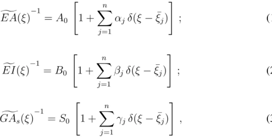
According to the flexibility modelling [7], the presence of a concentrated damage at the generic abscissa ξ = ¯ξ results in a positive impulse in the flexibility tions, which in turn can be mathematically represented with a Dirac’s delta func-tion δ(ξ − ξ¯) centred at the position of the damage. It follows that, if n cracks occur in the beam, axial flexibility EAg(ξ)−1 = E L2/EA(ξL), flexural flexibility
f
EI(ξ)−1 = E L4/EI(ξL) and shear flexibility GAg
s(ξ)
−1
= E L2/GA
s(ξL) take
the dimensionless expressions:
g
EA(ξ)−1 =A0 "
1 +
n
X
j=1
αjδ(ξ−ξ¯j)
#
; (1)
f
EI(ξ)−1 =B0 "
1 +
n
X
j=1
βjδ(ξ−ξ¯j)
#
; (2)
g
GAs(ξ)
−1
=S0 "
1 +
n
X
j=1
γjδ(ξ−ξ¯j)
#
, (3)
where ξ¯j is the dimensionless abscissa at the jth crack position, while A0 = L2/A,
B0 = L4/I andS0 = 2κ(1 +ν)L2/A are dimensionless constants,AandI being
the cross-sectional area and its principal second moment orthogonal to the bending plane, respectively, while κis the shear correction factor andνis the Poisson’s ratio; moreover, the dimensionless parametersαj, βj and γj define the intensity of thejth
impulses in the three flexibility functions, which in turn are related to severity of the corresponding longitudinal, rotational and transverse damages, i.e. the severer the damage, the higher are the impulses (while the condition αj = βj = γj = 0
corresponds to absence of damage atξ = ¯ξj).
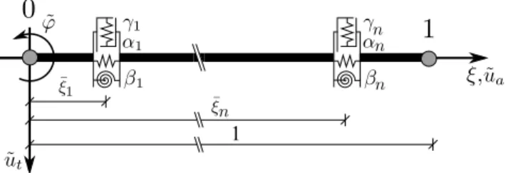
Figure 2 displays an-cracked prismatic beam element, with unitary length in the dimensionless system of reference, with discontinuities shown at ξ = ¯ξ1 andξ = ¯ξn,
where the first and the nth damage are located. The two ends of the MCB element are denoted with nodes0and1, and each cross section of the member possesses three degrees of freedom, i.e. the two axial and transverse translations,eua(ξ)andeut(ξ), and
1
Figure 2: Sketch of the two-node MCB element
2.2
Axial load
Let us consider first the case in which the dimensionless axial loadeqa(ξ)is distributed
along an-cracked beam. The exact closed-form solution in terms of the resulting field of dimensionless axial displacements eua(ξ) = ua(ξ L)/L has been derived, and can
be expressed as:
e
ua(ξ) =A0 "
C1ξ+C2−qea[2](ξ) + n
X
j=1
αj −eqa[1]( ¯ξj) +C1H(ξ−ξ¯j)
#
, (4)
in which the superscripted expression [i] denotes the ith primitive function, while H(ξ − ξ¯j) = δ[1](ξ −ξ¯j) is the Heaviside’s unit step function applied at ξ = ¯ξj;
moreover, C1 and C2 are two integration constants, whose values can be evaluated
once the boundary conditions (BCs) are enforced.
The first derivative of the axial displacement gives the axial deformation of the centroidal fibre:
e
εa(ξ) = eua′(ξ) =A0 "
C1−qea[1](ξ) + n
X
j=1
αj −eqa[1]( ¯ξj) +C1
δ(ξ−ξ¯j)
#
, (5) where the symbol ′ stands for the spatial derivative with respect to the dimension-less abscissa ξ, i.e. (·)′ = d (·)/dξ. It is worth emphasising here that the presence of a crack at the position ξ = ¯ξj results in a finite jump in terms of axial
displace-ments, represented by the Heaviside’s unit step function H(ξ −ξ¯j)in Equation (4),
and in an impulse in terms of the axial strain, represented by the Dirac’s delta function δ(ξ−ξ¯j)in Equation (5). These singularities disappear in the dimensionless normal
forceNe(ξ) = N(ξ L)/(E L2), as any concentration of stress atξ = ¯ξ
j is then
aver-aged over the whole cross section:
e
N(ξ) =EAg(ξ)eεa(ξ) =C1−eqa[1](ξ). (6)
2.3
Transverse load
Let us consider now the case in which the dimensionless transverse load qet(ξ)is
the kinematics of the uncracked portions of the beam. The resulting field of the di-mensionless transverse displacementsuet(ξ) = ut(ξ L)/L can be decomposed in
pure-bending (i.e. Euler-Bernoulli) contribution, ueb(ξ), and a pure-shearing contribution,
e
us(ξ), which are ruled by coupled differential equations.
By extending the formulation presented by Palmeri and Cicirello [7] to include the presence of a transverse spring at the position of the generic concentrated damage (see Equation (3)), the exact closed-form solution for this problem has been derived, and can be expressed in the form:
e
ut(ξ) = B0 1
6C3ξ
3 +1
2C4ξ
2+C
5ξ+C6−qet[4](ξ)
+ n X j=1 βj e
qt[2]( ¯ξj) +C3ξ¯j +C4
(ξ−ξ¯j)H(ξ−ξ¯j)
−S0
C3ξ+qet[2](ξ) + n
X
j=1
γj
C3+qet[1]( ¯ξj)
H(ξ−ξ¯j)
,
(7)
whereC3,C4,C5andC6 are four integration constants, to be determined by imposing
the relevant BCs.
The spatial derivative of Equation (7) with respect to the dimensionless abscissa ξ gives the slope function of the beam, which takes into account both bending and shearing contributions, while taking the derivative of the sole bending term (i.e. the first two lines in the r.h.s. of Equation (7)) delivers the rotation of the cross section, with opposite sign to take into account the adopted system of reference (see Figure 2), that is:
e
ϕ(ξ) =−ue′
b(ξ) =−B0 1
2C3ξ
2+C
4ξ+C5+qet[3](ξ)
+ n X j=1 βj e
qt[2]( ¯ξj) +C3ξ¯j +C4
H(ξ−ξ¯j)
.
(8)
The dimensionless bending curvature of the beam is obtained by taking the spatial derivative of the Equation (8) with respect to the dimensionless abscissaξ:
e
χ(ξ) = ϕe′(ξ) =−B 0
C3ξ+C4+qet[2](ξ)
+ n X j=1 βj e
qt[2]( ¯ξj) +C3ξ¯j +C4
δ(ξ−ξ¯j)
,
(9)
while the average shearing strain is given by:
e
Γ(ξ) =ue′
t(ξ) +ϕe(ξ) =−S0
C3+eqt[2](ξ) + n
X
j=1
γj
C3+eqt[1]( ¯ξj)
δ(ξ−ξ¯j)
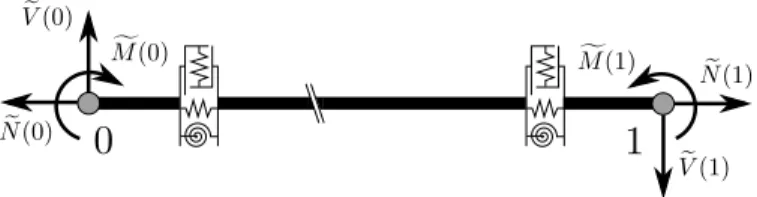
Figure 3: Dimensionless internal forces at the two end nodes of the MCB element Interestingly, like in the case of the axial load, the two measures of the deformation introduced for the transverse load, i.e. the dimensionless bending curvature of Equa-tion (9) and the average shearing strain of EquaEqua-tion (10), show impulsive terms at the position of the generic crack, which are proportional to the corresponding dimension-less measures βj and γj of the severity of the damage. These impulses disappear in
the expressions of the associated internal forces, i.e. the dimensionless bending mo-ment bending momo-mentMf(ξ) = M(ξ L)/(E L3), positive if sagging, and shear force
e
V(ξ) = V(ξ L)/(E L2), respectively: f
M(ξ) =EIf(ξ)χe(ξ) = −C3ξ−C4−qet[2](ξ) ; (11)
e
V(ξ) =GAgs(ξ)eΓ(ξ) = −C3−qet[1](ξ) = Mf′(ξ). (12)
Figure 3 illustrates the positive sign convention for the dimensional internal forces
e
N(ξ), Ve(ξ) and Mf(ξ) at the position of the two end nodes 0 (at ξ = 0) and 1 (at ξ = 1), which will be used in the next Section to derive the elements of stiffness matrix and equivalent load vector.
3
Multi-cracked beam (MCB) element
The closed-form exact solutions for a beam withn cracks under axial and transverse loads, as presented in the previous Section, allows the direct definition of the(6×6)
dimensionless stiffness matrixKe by evaluating the dimensionless internal forces at the
two end nodes due to a unit settlement imposed to a single nodal degree of freedom (DoF) per time, while the other BCs are zeroed and the beam is unloaded, i.e.qea(ξ) =
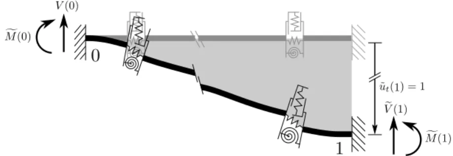
0 andqet(ξ) = 0. For illustration purposes, Figure 4 shows the deformed shape of a
multi-cracked beam due to a unit transverse settlement at the end node 1, with finite jumps in the transverse displacement and rotation at the position of the cracks.
The generalised Hooke’s law,Feu = Ke ·eu, has been therefore exploited, in which
e
Fu is the array of the nodal forces (expressed in a global system of reference):
e
Fu =n−Ne(0),−Ve(0),−Mf(0),Ne(1),Ve(1),Mf(1)o⊤ ; (13)
andeuis the array of the corresponding DoFs:
e
Figure 4: Deformed shape for a unit transverse settlement
the superscripted symbol⊤meaning the transpose operator. In this way, each column of the stiffness matrixKe is given by the arrayFeucomputed for a unit settlement of the
associated DoF, e.g. the shear forces and bending moments represented within Figure 4 are the elements of the fifth column (uet(1) = 1) of the sought matrixKe.
Moreover, the axial displacement functionuea(ξ) and the transverse displacement
functioneut(ξ)so computed can be adopted as shape functions to evaluate the
dimen-sionless mass matrixMf.
The array Feq of the equivalent nodal forces for a generic distribution of actual
loads qea(ξ) and qet(ξ) acting on the MCB element can be determined with the help
of the same closed-form exact solutions reported in the previous Section, by taking zeroed BCs and evaluating the corresponding internal forces at the two end nodes:
e
Fq =nNe(0),Ve(0),Mf(0),−Ne(1),−Ve(1),−Mf(1)o⊤ , (15)
in which the signs in the r.h.s. are opposite with respect to Equation (13) because of the action-reaction principle.
Since the axial and transverse components are decoupled, the respective formula-tions can be treated separately, by using the same approach. Due to the limitaformula-tions in the length of the paper, however, only the formulation for the axial component will be developed in the following Subsections.
3.1
Axial stiffness matrix
The relationship between axial displacements and forces for the MCB under consid-eration can be posed in the form:
e
Fu(a) =Ke(a)·eu(a), (16)
where the(2×1)arraysFe(a)=−Ne(0),Ne(1) ⊤andeu(a)=uea(0),uea(1) ⊤collect
the relevant elements ofFeuanduegiven by Equations (13) and (14), respectively, while
the elements of the (2×2)matrixKe(a) correspond to the elements of the matrixKe
associated with the axial component, that is:
h e
Kai
(r+2)/3,(s+2)/3 = h
e
Ki
in which the notation [·]r,s means the element of the matrix within square brackets taken from rth row and sth column, and the condition {r, s} ⊆ {1,4}must be sat-isfied, meaning that first and fourth rows and columns of the stiffness matrix Ke are
those associated with the axial component.
By following the procedure summarised above, the first column of the matrixKe(a),
obtained fors = 1, can be obtained by taking the values of the dimensionless normal forceNe(1)(0)andNe(1)(1)at the two end nodes0and1for the BCseu(1)
a (0) = 1and
e
ua(1)(1) = 0 and zeroed axial loadeqa(ξ) = 0, while the transverse component is
ne-glected. It is therefore possible to evaluate the values of the two integration constants C1(1) andC2(1) appearing in the r.h.s. of Equation (4), which in turn allow calculating the dimensional normal force through Equation (6). It can be easily verified that for this case:
e
N(1)(0) = Ne(1)(1) =−hKei
1,1 = h
e
Ki
4,1 =−A
−1
0 (1 +a0)−1 , (18)
where the superscripted notation(1)means that the first DoF in the arrayeuof Equation
(14) is being considered, and the new dimensionless quantity a0 = Pnj=1αj is an
overall measure of the additional axial flexibility due to the presence of thencracks. Similarly, for the second column of the matrix Ke(a), obtained fors = 4 and having
reversed BCs, one obtains:
e
N(4)(0) =Ne(4)(1) =−hKei
4,1 = h
e
Ki
4,4 =A
−1
0 (1 +a0)−1 . (19)
The results of Equations (18) and (19) allow thus building the stiffness matrixKe(a):
e
Ka =A−1
0 (1 +a0)−1
1 −1
−1 1
. (20)
It is worth nothing that for a0 = 0, Equation (20) gives the (2×2) dimensionless
stiffness matrix of an undamaged uniaxial bar.
3.2
Uniform axial load
In order to provide an example of how the array of the equivalent nodal forces can be computed, the case of a uniformly distributed axial loads is considered in this Sub-section. The same procedure adopted for the stiffness matrix can be applied, with the only difference that this time the BCs are all zeroed, i.e. uea(0) = 0anduea(1) = 0,
and qea(ξ) = eqa. After some algebra, the values of the normal force at the two end
nodes can be expressed as:
e
N(0) =qea
1 + 2a1
2 (1 +a0)
; Ne(1) =−eqa
1 + 2 (a0−a1)
2 (1 +a0)
, (21) wherea1 = Pnj=1αjξ¯j represents the dimensionless first moment of the coefficients
3.3
Axial mass matrix
To perform the FE analysis a of a multi-cracked beam subjected to dynamic load-ing, the dimensionless mass matrix Mf, consistent with the dimensionless stiffness
matrix Ke, is highly desirable. However, little attention has been paid in the past to
this issue, and the approximation of lumped masses has been generally adopted (e.g. Reference [19]), therefore neglecting the effects of the damaged cross sections on the inertial forces experienced by the MCB element. Indeed, when the approximation with lumped masses is resorted to, the mass of the whole FE is concentrated at the two end nodes, like in the uncracked beam, despite the fact that the damage on the member can significantly alter the distribution of the inertial forces. It will be shown in the next Section that the implementation of the lumped mass matrix in conjunction with a MCB element reduces (and potentially nullifies) most of the computational ad-vantage of such formulation for applications of Structural Dynamics, as more FEs are required to capture the eigenproperties (modal shapes and modal frequencies) of the cracked beam.
To the best of our knowledge, Caddemi et al. [20] have been the first researchers to address this issue, as they have used a MCB element with a consistent mass matrix to carry out the modal analysis of a 3D linear elastic frame with damage concentrated at various locations. Although their mathematical derivation involves the rigidity mod-elling to represent the concentrated damage in the MCB element [5, 6], the proposed approach, based on the alternative (and physically consistent) flexibility modelling [7], delivers the same results.
In order to evaluate the consistent mass matrix for the problem in hand, the same deformed shapes derived by assigning unit settlements at the two end nodes of the MCB element have been used, meaning that the same set of shape functions discretise both potential and kinetic energy of the FE. For the axial component, the dimension-less(2×2)consistent mass matrix can be evaluated as:
f
Ma=A−1
0 Z 1
0 e
ha(ξ)·eha(ξ)⊤dξ , (22)
where the mass density of the materialρhas been selected as third dimensional refer-ence variable of the problem, and therefore it does not appear in the above expression, whilehea(ξ) = uea(1)(ξ), uea(4)(ξ) ⊤ is the(2×1)array collecting the dimensionless
functions representing the axial displacements in the MCB for unit axial settlements at end nodes0and1.
If follows from Equation (22) that for evaluating the generic element of the mass matrixfMa, the following integral must be computed:
h f
Mai
r,s =A
−1
0 Z 1
0 e
ua(r)(ξ)uea(s)(ξ) dξ , (23) with {r, s} ⊆ {1,4}, and for this purpose each shape function eua in the r.h.s. of
obtained when all the coefficientsαj are zeroed and therefore the beam is assumed to
be uncracked, andnadditional terms,ga,j, each one contributing forξ ≥ ξ¯j. That is,
for therth axial shape function, one can write:
e
ua(r)(ξ) = A0 fa(r)(ξ) + n
X
j=1
ga,j(r)(ξ)
!
, (24)
where (see Equation (4)):
fa(r)(ξ) = C1(r)ξ+C2(r); (25)
ga,j(r)(ξ) =αjC1(r)H(ξ−ξ¯j). (26)
Substitution of Equation (24) into Equation (23) leads to:
h f
Mai
r,s=A0
Z 1 0
fa(r)(ξ)fa(s)(ξ) +
n
X
j=1
fa(r)(ξ)ga,j(s)(ξ)
+
n
X
j=1
fa(s)(ξ)ga,j(r)(ξ) +
n X j=1 n X k=1
ga,j(r)(ξ)ga,k(s)(ξ)
!
dξ ,
(27)
and each term in the r.h.s. can be evaluated in closed-form:
Z 1 0
fa(r)(ξ)fa(s)(ξ) dξ= 1 3C
(r)
1 C
(s)
1 +
1 2
C2(r)C1(s)+C1(r)C2(s)+C2(r)C2(s) ; (28)
Z 1 0
fa(r)(ξ)ga,j(s)(ξ) dξ =αjC1(s) C (r) 1
1−ξ¯2
j
2 +C
(r)
2 (1−ξ¯j)
!
; (29)
Z 1 0
ga,j(r)(ξ)ga,k(s)(ξ) dξ =αjαkC1(r)C (s)
1 ξ¯j,k(1−ξ¯j,k), (30)
withξ¯i,k = maxξ¯j, ξ¯k .
3.4
Transverse component
The same approach presented in the previous three Subsections for the axial displace-ment eua(ξ) can be adopted for the transverse displacement eut(ξ). The expressions
of the stiffness coefficients, equivalent nodal forces and consistent mass coefficients become more complicated because: i) the transverse deflection of the beam is the superposition of its pure-bending component, ueb(ξ), and pure-shearing component,
e
us(ξ);ii) the field of pure-bending displacementsueb(ξ)is ruled by a fourth-order
dif-ferential equation, as opposite to the second-order difdif-ferential equation foruea(ξ), and
therefore four integrations constants appear in the solution (see Equation (7)).
Interestingly, it can be shown that while for the axial component the dimensionless stiffness coefficients of the MCB element depends on the constants A0 (normalised
axial flexibility of the uncracked member) and a0 (total additional flexibility arising
from the n cracks at different locations), the dimensionless stiffness coefficients for transverse component depends onB0andS0 (i.e. the dimensionless constants playing
the same role as A0 for the pure-bending and pure-shearing deflection), along with
the additional dimensionless quantities bm = Pnj=1βjξ¯m, with m ∈ {0,1,2}, and
c0 =Pnj=1γj.
4
Numerical applications
In this Section, the performance of the proposed MCB element has been tested by means of two numerical applications, namely:i) a slender (Euler-Bernoulli) cantilever beam with two cracks (n= 2) subjected to concentrated and uniform distributed loads, inducing both axial and transverse displacements (Section 4.1);ii) a planar frame with two cracks and subjected to both vertical and lateral loads (Section 4.2), in which the contribution of the shear deformations have been also taken into account (Timoshenko beam theory).
In each example, the response analysis of the objective structure to the given static loads has been carried out by implementing the proposed MCB element within a MAT-LAB FE code, and it has been verified that the results so obtained with a single FE per member coincide with those delivered by the commercial FE code SAP2000 when at the position of each crack two additional nodes are introduced and connected by axial and/or rotational and/or transverse spring simulating the residual stiffness of the damaged section. The exact static response of these two DS models have been also compared with the approximate one computed by implementing the LSR model with an increasing number of elements per member. In both examples, the static analy-sis has been followed by a dynamic (modal) analyanaly-sis of the nude objective structure, looking at the convergence of different FE models in terms of the first few modal fre-quencies of vibration, which has once again demonstrated the improved performance of the proposed MCB element.
4.1
Slender cantilever beam
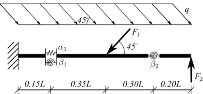
In the first application, a slender cantilever beam of lengthL= 1.00m has been stud-ied. The beam is made of steel, with Young’s modulusE = 210GPa and Poisson’s ratio ν = 0.30, and the cross section is a solid square with dimensions of 50×50
mm. As shown within Figure 5, two cracks are assumed at the abscissas x = 0.15L and x = 0.80L; the first crack is modelled with a longitudinal spring of stiffness Ka = 5,250kN/mm in series with a rotational springKr = 1,094 kN×m,
corre-sponding to the dimensionless damage parameters α1 =β1 = 0.1, while the second
crack simply consists of a rotational spring, having the same stiffnessKrand therefore
the same dimensionless parameterβ2 = 0.1.
Figure 5: Multi-cracked cantilever beam (first example)
loads have been considered in this case (see Figure 5): a uniformly distributed load q = 3.0√2 kN/m, forming an angle of45◦ with the longitudinal axis of the beam;
a first point force F1 = 20.0
√
2 kN, inclined by 45◦ and applied at the midspan
position; a second point forceF2 = 7.0kN, applied upward at the free end.
The results in terms of dimensionless displacements and rotation at the free end of the cantilever beam are compared in Table 1 for three different methods of analysis, showing that the DS model with the proposed MCB formulation and just 1 FE is in perfect agreement with the conventional DS model built with SAP2000, which however requires 3 FEs; while the LSR model with 5 FEs is still affected by significant inaccuracies, i.e. the transverse deflection at the free end is overestimated by about 30%, and the slope at the same point is underestimated by about 20%.
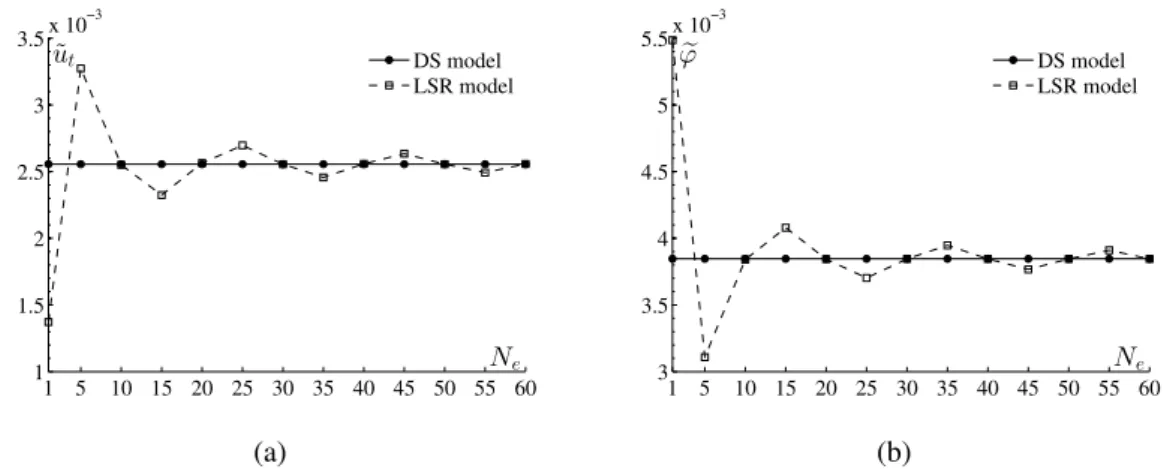
This aspect has ben further investigated, and Figure 6 shows the convergence of the LSR model (dashed line) to the exact solution (solid line) as the number Ne of FEs
used to discretise the multi-cracked beam increases. The same two response parame-ters have been considered, and it can be observed that in both cases the convergence is oscillatory, as the exact solution can be either underestimated or overestimated by the LSR model, depending on the adopted mesh. Interestingly, more than 50 FEs are required for the LSR model to deliver accurate results, the reason being that the as-sumption of concentrated damage means that the increase in the flexibility of the beam is distributed over a very small region, and a conventional FE formulation can achieve this only with a very fine mesh. On the contrary, the proposed MCB element gives the exact results independently of the number of element used in the mesh.
Figure 7(a) and 7(b) displays the deformed shape (left column) and the slope func-tion (right column) of the cantilever beam as computed with 5 FEs (top row) and 15
e
ua(1) uet(1) ϕe(1)
DS Proposed (1 FE) -1.9514×10⁻⁵ -2.5561×10⁻³ 3.8457×10⁻³
DS SAP2000 (3 FEs) -1.9514×10⁻⁵ -2.5561×10⁻³ 3.8457×10⁻³
LSR Model (5 FEs) -1.9486×10⁻⁵ -3.2741×10⁻³ 3.1086×10⁻³
1 5 10 15 20 25 30 35 40 45 50 55 60 1 1.5 2 2.5 3
3.5x 10
−3
Ne ˜
ut DS model
LSR model
(a)
1 5 10 15 20 25 30 35 40 45 50 55 60
3 3.5 4 4.5 5
5.5x 10
−3
Ne
e
ϕ DS model
LSR model
(b)
Figure 6: Convergence in terms of transverse deflection (a) and rotation (b) at the free end (first example)
FEs (bottom row). In these graphs, the DS model (solid lines), implemented with the proposed MCB element, represents the exact solution, as increasing the number Ne
of FEs just reduces the sampling interval, but does not change the values at a given abscissa, e.g. deflection and rotation at the free end do not vary with the meshing size. On the contrary, the approximate solution computed with the LSR model improves with the number of FEs.
In a second stage, the modal analysis of the same multi-cracked slender beam has been carried out. The attention has been focussed on the transverse vibration of the beam, for which Caddemi and Cali`o [21] have recently provided the exact closed-form solutions in terms of eigenproperties, i.e. modal frequencies and modal shapes, by adopting the Euler-Bernoulli beam theory.
Table 2 compares the exact values of the first five modal frequencies with those computed with 5 FEs and four different approximate models, namely: the DS model with the proposed MCB element and both consistent and lumped mass matrices; the DS model implemented in the commercial FE software SAP2000; the LSR model
0 0.25 0.5 0.75 1
0
2
4 x 10⁻³
ξ
˜
ut
0 0.25 0.5 0.75 1
0
2
4 x 10⁻³
ξ ˜ ut DS LSR DS LSR (a)
0 0.25 0.5 0.75 1
−10 −5 0 5x 10
−3
ξ ˜
ϕ
0 0.25 0.5 0.75 1
−10 −5 0 5x 10
−3 ξ ˜ ϕ DS LSR DS LSR (b)
Figure 7: Fields of transverse displacements (a) and rotations (b) when 5 (top) and 15 (bottom) FEs are used to discretise the beam (first example)
1st mode 2nd mode 2 3rd mode 4th mode 5th mode Exact [21] 37.31 253.56 682.06 1279.14 2115.28 DS Consistent 37.31 253.73 684.08 1290.97 2154.85 DS Lumped 36.67 236.28 590.99 1082.04 1687.81 DS SAP2000 36.67 236.28 590.99 1082.04 1687.81 LSR Model 35.95 226.20 605.20 1127.16 1694.44 Table 2: Modal frequencies [Hz] of the cantilever beam discretised with 5 elements (first example)
1 2 3 4 5 6 7 8 9 10
102 103
Frequency [Hz]
Ne DS Lumped DS Consistent DS Theoretical LSR Lumped
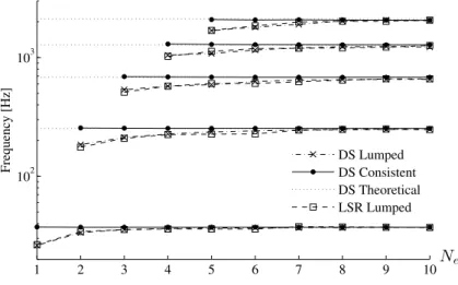
Figure 8: Frequencies convergence diagram (first example)
with lumped masses. The results of the proposed MCB element with consistent mass matrix are in excellent agreement with the exact results (that is, the inaccuracy is virtually negligible in the first mode of vibration, and is less than 2% in the fifth mode), while using the lumped mass matrix affects significantly the accuracy (the first modal frequency is underestimated by about 2%, while the inaccuracy in the fifth modal frequency is as large as 20%). The FE analysis carried out with SAP2000 delivers exactly the same results as the proposed MCB element with lumped mass matrix, as the same mesh has been adopted for validation purposes. Interestingly, the same level of inaccuracy is shown by the LSR model with lumped masses, which therefore appears as a very crude approximation for dynamic applications.
This is confirmed by the semi-log convergence diagram of Figure 8, showing that the DS model with the proposed MCB element and consistent mass matrix (solid lines) is able to accurately estimate the first n modal frequencies with justn FEs. All the other models, adopting lumped masses, are less efficient and require at least2n FEs to provide an accurate estimation of thenth modal frequencies.
0.50L
0.40L 0.60L
A B
C
D
L
0.25L
Figure 9: Multi-cracked portal frame (second example)
4.2
Portal frame
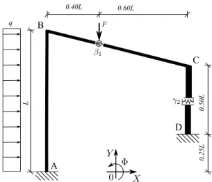
A similar trend of results has been observed for the static and dynamic analysis of the portal frame with sloping beam shown within Figure 9. The frame is L= 4 m wide, while the first columnABis4 m tall and the second columnCDhas half the height; the slope of the top beam is 1:4, and the fixed end D of the second column is raised by
1 m. The material properties are the same as in the previous example; the cross section of column AB and beam BC is a solid rectangle, 50 mm wide and 150 mm deep, while the cross section of the columnCD has twice the width, and in both cases the shear correction factor isκ= 1.2. The frame has two concentrated damages: the first one, modelled as a rotational spring of stiffnessKr = 71,624kN×m (corresponding
toβ1 = 0.01), occurs on the top beam at the abscissax = 0.40L, taken from the left
end B; the second damage is represented by a shear spring of stiffness Ks = 50.48
kN/mm and occurs at mid-height of the second column.
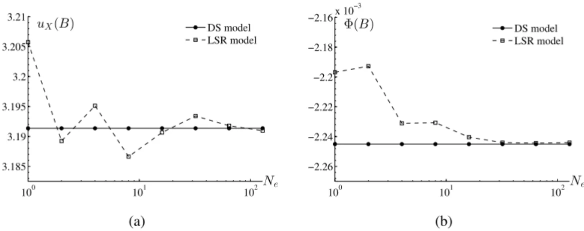
The static analysis has been carried out with the two loads shown in Figure ref-fig:Example2, namely a lateral uniform load q = 10 kN/m distributed on the first column and a point forceF =q×L= 40kN at the cracked section on the top beam. The semi-log Figure 10 shows the convergence of the LSR model while increasing the numberNeof FEs used per each member. Like in the case of the cantilever beam
stud-ied in the previous Subsection, the convergence is slow and quite irregular, particularly forNe<50.
The modal analysis of the nude portal frame has been also performed, confirming the superior performance of the proposed MCB element with consistent mass matrix. The semi-log Figure 11 shows that with Ne = 2(i.e. two FEs per member and six
in total) the proposed model (solid lines) accurately predicts the first three modal fre-quencies, while withNe= 2(i.e. three FEs per member and nine in total), the analysis
converges also for the fourth and fifth modal frequency. More FEs are needed for two models with lumped masses, showing also in this circumstance a slower convergence.
100 101 102 3.185
3.19 3.195 3.2 3.205 3.21
Ne
uX(B) DS model
LSR model
(a)
100 101 102
−2.26 −2.24 −2.22 −2.2 −2.18
−2.16x 10
−3
Ne
Φ(B) DS model
LSR model
(b)
Figure 10: Convergence in terms of horizontal displacement (a) and rotation (b) at node B (second example)
5
Conclusions
A two-node MCB (multi-cracked beam) element for the static and dynamic analysis of planar framed structures with concentrated damages has been presented and numer-ically tested. The proposed model follows the DS (discrete spring) representation of (linear elastic) always-open cracks, in which the beam is fully articulated at the po-sition of each crack, and a set of axial, rotational and transverse elastic springs takes into account the residual stiffness of the damaged section, while axial, bending and shear deformations are considered in the undamaged regions of the beam between two consecutive singularities (i.e. the end nodes and the cracked sections).
The (physically consistent) flexibility modelling of the concentrated damage has been adopted to derive the exact closed-form expressions for the deformed shape and
1 2 3 4 5 6 7 8 9 10
101 102
Frequency [Hz]
Ne DS Lumped DS Consistent LSR Lumped
internal forces of a beam withncracks of arbitrary severity and position, subjected to static axial and transverse loading. By exploiting the generalised Hooke’s law and the action-reaction principle, these results have been used to determine the dimensionless stiffness matrix and array of equivalent nodal forces. The consistent mass matrix has been also computed, by adopting the same shape functions to represent the inertial forces on the MCB element.
Unlike the conventional DS models, which require the beam to be split at the posi-tion of each crack, with two FE nodes added to both sides of each crack, the proposed MCB element embeds the effects of the concentrated damages without enlarging the size of the FE model. It follows that the exact static solution is retrieved independently of the mesh, while a faster convergence is achieved for the dynamic problems. This has been confirmed with two numerical examples, which also demonstrate the improved performance of the proposed MCB element in comparison with the approximate LSR (local stiffness reduction) approach, very often used for problems of damage detec-tion.
It must be stressed that the proposed MCB element is equivalent to the analogous FE formulation recently proposed by other researchers (see Reference [20]), which however have used the (physically inconsistent) rigidity modelling of the concentrated damage.
References
[1] M.I. Friswell and J.E.T. Penny, “Crack modeling for structural health monitor-ing”, Structural Health Monitoring, 1, 139-148, 2002.
[2] D. Capecchi and F. Vestroni, “Damage evaluation in cracked vibrating beams using experimental frequencies and finite element models”, Journal of Vibration and Control, 2, 69-86, 1996.
[3] D. Capecchi and F. Vestroni, “Damage detection in beam structures based on fre-quency measurements”, Journal of Engineering Mechanics, 126, 761-768, 2000. [4] F. Vestroni and M.N. Cerri, “Detection of damage in beams subjected to diffused
cracking”, Journal of Sound and Vibration, 234, 259-276, 2000.
[5] B. Biondi and S. Caddemi, “Closed form solutions of Euler-Bernoulli beam with singularities”, International Journal of Solids and Structures, 42, 3027-3044, 2005.
[6] B. Biondi and S. Caddemi, “Euler-Bernoulli beams with multiple singularities in the flexural stiffness”, European Journal of Mechanics - A/Solids, 26, 789-809, 2007.
[7] A. Palmeri and A. Cicirello, “Physically-based Diracs delta functions in the static analysis of multi-cracked Euler-Bernoulli and Timoshenko beams”, International Journal of Solids and Structures, 48, 2184-2195, 2011.
[8] A.D. Dimarogonas, “Vibration of cracked structures: a state of the art review”, Engineering Fracture Mechanics, 55, 831-857, 1996.
[9] G.R. Irwin. “Analysis of stresses and strains near the end of a crack traversing a plate”, Journal Applied Mechanics, 24, 361-364, 1957.
[10] P.G. Kirmsher, “The effects of discontinuities on the natural frequency of a beams”, Proceedings American Society of Testing and Materials, 44, 897-904, 1944.
[11] P. Cacciola, N. Impollonia and G. Muscolino, “Crack detection and location in a damaged beam vibrating under white noise”, Computer and Structures, 81, 1773-1782, 2003.
[12] S. Caddemi, I. Cali`o and M. Marletta, “The non-linear dynamic response of the Euler-Bernoulli beam with an arbitrary number of switching cracks”, Interna-tional Journal of Non-Linear Mechanics, 45, 714-726, 2010.
[13] R. Ghanem and M. Shinozuka, “Structural-system identification. I: Theory”, Journal of Engineering Mechanics, 121, 255-264, 1995.
[14] S. W. Doebling, C. R. Farrar and M. B. Prime, “A Summary Review of Vibration-Based Damage Identification Methods”, The Shock and Vibration Digest, 30, 91-105, 1998.
[15] C. R. Farrar, S. W. Doebling and D. A. Nix, “Vibrationbased structural damage identification”, International Journal for Numerical Methods in Engineering, 45, 131-149, 2001.
[16] C. Cremona and A. Alvandi, “Assessment of vibration-based damage identifica-tion techniques”, Journal of Sound and Vibraidentifica-tion, 292, 179-202, 2006.
[17] G. Buda and S. Caddemi, “Identification of concentrated damages in Euler-Bernoulli beams under static loads”, Journal of Engineering Mechanics, 133, 942-956, 2007.
[18] P. Cacciola, N. Maugeri and G. Muscolino, “Structural identification through the measure of deterministic and stochastic time-domain dynamic response”, Com-puter and Structures, 89, 1812-1819, 2011.
[19] M. Skrinar, “Elastic beam finite element with an arbitrary number of transverse cracks”, Finite Element in Analysis and Design, 45, 181-189, 2009.
[20] S. Caddemi, I. Cali`o and D. Rapiacavoli, “The influence of concentrated damage in the dynamic behaviour of framed structures”, L’Ingegneria Sismica in Italia, ANIDIS 201, 2011.
[21] S. Caddemi, I. Cali`o “Exact closed-form solution for the vibration modes of the EulerBernoulli beam with multiple open cracks” Journal of Sound and Vibration, 327, 473489, 2009.