LEARNING FROM COMPLEX NEUROIMAGING DATASETS
Mahmoud Mostapha
A dissertation submitted to the faculty of the University of North Carolina at Chapel Hill in partial fulfillment of the requirements for the degree of Doctor of Philosophy in the Department of
Computer Science.
Chapel Hill 2020
ABSTRACT
Mahmoud Mostapha: Learning from Complex Neuroimaging Datasets (Under the direction of Martin A. Styner)
Advancements in Magnetic Resonance Imaging (MRI) allowed for the early diagnosis of neu-rodevelopmental disorders and neurodegenerative diseases. Neuroanatomical abnormalities in the cerebral cortex are often investigated by examining group-level differences of brain morphometric measures extracted from highly-sampled cortical surfaces. However, group-level differences do not allow for individual-level outcome prediction critical for the application to clinical practice.
Despite the success of MRI-based deep learning frameworks, critical issues have been identified: (1) extracting accurate and reliable local features from the cortical surface, (2) determining a parsimonious subset of cortical features for correct disease diagnosis,(3)learning directly from a non-Euclidean high-dimensional feature space,(4)improving the robustness of task multi-modal models, and(5)identifying anomalies in imbalanced and heterogeneous settings.
This dissertation describes novel methodological contributions to tackle the challenges above. First, I introduce a Laplacian-based method for quantifying local Extra-Axial Cerebrospinal Fluid (EA-CSF) from structural MRI. Next, I describe a deep learning approach for combining local EA-CSF with other morphometric cortical measures for early disease detection. Then, I propose a data-driven approach for extending convolutional learning to non-Euclidean manifolds such as cortical surfaces. I also present a unified framework for robust multi-task learning from imaging and non-imaging information. Finally, I propose a semi-supervised generative approach for the detection of samples from untrained classes in imbalanced and heterogeneous developmental datasets.
ACKNOWLEDGMENTS
TABLE OF CONTENTS
LIST OF TABLES . . . x
LIST OF FIGURES . . . xi
LIST OF ABBREVIATIONS . . . xv
1 INTRODUCTION . . . 1
1.1 Overview . . . 1
1.2 Motivating Problems and Proposed Solutions . . . 6
1.2.1 Current Findings on Early Prediction of ASD from Neuroimaging Studies . . 6
1.2.2 Deep Convolutional Learning on Non-Euclidean Cortical Surfaces . . . 7
1.2.3 Deep Multi-Modal Multi-Task Learning for Robust Representation Learning 10 1.2.4 Deep Generative Models for Anomaly Detection in Heterogeneous Datasets 12 1.3 Thesis Statement . . . 15
1.4 Overview of Chapters . . . 17
2 BACKGROUND . . . 18
2.1 Overview of Deep Learning in Structural MRI Processing and Analysis . . . 18
2.2 Cortical Surface Reconstruction and Shape Analysis . . . 26
2.2.1 Cortical Surface Reconstruction . . . 26
2.2.2 Differential Geometry on Surfaces . . . 29
2.2.3 Cortical Surface Proprieties . . . 33
2.3 Common Deep Learning Architectures . . . 38
3.1 Overview . . . 49
3.2 Methods . . . 53
3.2.1 Materials . . . 53
3.2.2 Image Processing and Surface Generation . . . 54
3.2.3 Extraction of Local Extra-Axial Cerebrospinal Fluid . . . 57
3.3 Experimental Results . . . 61
3.4 Summary . . . 67
4 EARLY PREDICTION OF AUTISM SPECTRUM DISORDER . . . 69
4.1 Introduction . . . 69
4.2 Methods . . . 73
4.2.1 Materials . . . 73
4.2.2 Image Processing and Surface Generation . . . 75
4.2.3 Feature Extraction . . . 77
4.2.4 Deep Learning Prediction . . . 80
4.3 Experimental Results . . . 83
4.4 Summary and Discussion . . . 94
5 CONVOLUTIONAL LEARNING ON CORTICAL BRAIN SURFACES . . . 97
5.1 Overview . . . 97
5.2 Methods . . . 101
5.2.1 Convolutional Learning on Surfaces . . . 101
5.2.2 Surface Subsampling . . . 104
5.3 Experimental Results . . . 105
5.3.1 Alzheimer’s Disease Classification . . . 106
5.3.1.1 Materials . . . 106
5.3.1.2 Data Preprocessing . . . 106
5.3.1.4 Performance Evaluation . . . 108
5.3.2 Early Prediction of Autism . . . 112
5.3.2.1 Materials . . . 112
5.3.2.2 Data Preprocessing . . . 112
5.3.2.3 Network Architecture and Training . . . 114
5.3.2.4 Performance Evaluation . . . 115
5.4 Summary . . . 116
6 ROBUST MULTI-TASK MULTI-MODAL DEEP LEARNING . . . 118
6.1 Overview . . . 118
6.2 Methods . . . 123
6.2.1 Multi-Modal Learning Block . . . 123
6.2.2 Multi-Modal Segmentation Networks . . . 124
6.2.3 Multi-Task Multi-Modal Network . . . 125
6.3 Experimental Results . . . 127
6.3.1 MRI Tissue Segmentation . . . 127
6.3.1.1 Materials . . . 127
6.3.1.2 Data Preprocessing . . . 129
6.3.1.3 Networks Architecture and Training . . . 131
6.3.1.4 Performance Evaluation . . . 131
6.3.2 Alzheimer’s Disease Classification and Cognitive Scores Prediction . . . 133
6.3.2.1 Materials . . . 133
6.3.2.2 Data Preprocessing . . . 135
6.3.2.3 Network Architecture and Training . . . 136
6.3.2.4 Performance Evaluation . . . 137
6.4 Summary . . . 139
7.1 Overview . . . 140
7.2 Methods . . . 143
7.2.1 Variational Autoencoder . . . 144
7.2.2 Generative Adversarial Network . . . 144
7.2.3 Semi-Supervised VAE-GAN for Out-of-Sample Detection . . . 145
7.3 Experimental Results . . . 150
7.3.1 Materials . . . 150
7.3.2 Model Architecture . . . 152
7.3.3 Performance Evaluation . . . 154
7.4 Summary . . . 158
8 SUMMARY AND CONCLUDING DISCUSSION . . . 159
8.1 Summary of Contributions . . . 159
8.2 Limitations. . . 165
8.3 Future Work . . . 166
8.3.1 Computational and Design Issues . . . 166
8.3.2 Clinical Applications . . . 168
LIST OF TABLES
3.1 Demographic information of longitudinal IBIS dataset . . . 54
4.1 Demographic information of six months IBIS dataset. . . 74
4.2 Autism prediction results using independent cortical measures . . . 88
4.3 Autism prediction results using combinations of cortical measures . . . 91
4.4 Autism prediction results in the general low-risk population . . . 93
5.1 AD classification results using cortical measures . . . 110
5.2 Autism prediction results using subcortical measures . . . 116
6.1 Multi-modal networks key parameters . . . 131
6.2 Multi-modal networks segmentation results . . . 132
6.3 Multi-task multi-modal network key parameters . . . 137
6.4 Multi-task multi-modal network prediction results . . . 138
7.1 Anomaly detection framework architecture . . . 153
LIST OF FIGURES
1.1 Proposed contributions in the MRI processing and analysis pipeline . . . 5
2.1 Structural T1-weighted MRI scan of a two-year-old infant . . . 18
2.2 Longitudinal MRI scans of a typically-developing infant . . . 19
2.3 MRI-based pipeline for early prediction of neurodevelopmental disorders . . . 20
2.4 Relationship between deep learning, machine learning, and artificial intelligence . . . 21
2.5 Architectures of feed-forward fully-connected neural networks . . . 22
2.6 Longitudinal cortical surfaces of a typically-developing infant . . . 28
2.7 The definition of the normal curvature on a smooth surface . . . 29
2.8 Shape characteristics of different curvature metrics . . . 31
2.9 Illustration of geodesics and shortest path on a smooth surface . . . 32
2.10 The connection between cortical thickness, surface area, and volume . . . 33
2.11 Illustration of the surface complexity index computation . . . 37
2.12 Generative versus discriminative learning approaches . . . 38
2.13 Convolutional neural networks control fundamental mechanisms . . . 40
2.14 AlexNet convolutional neural network architecture . . . 41
2.15 A fully convolutional network for infant tissue segmentation . . . 44
2.16 The architecture of a U-Net for medical image segmentation . . . 45
2.17 Illustration of a four-layer dense block . . . 45
2.18 Autoencoder and variational autoencoder networks architecture . . . 46
2.19 Generative adversarial network architecture . . . 48
3.1 Illustration of cerebrospinal fluid circulation . . . 50
3.2 Enlargement of extra-axial cerebrospinal fluid in an autistic infant . . . 51
3.3 Proposed framework for the extraction of local extra-axial cerebrospinal fluid . . . 53
3.5 Cortical surfaces reconstructed from input structural infant MRI . . . 56
3.6 The process of generating six-month cortical surfaces . . . 57
3.7 The solution of Laplace equation with two different boundary conditions . . . 58
3.8 The streamlines generated using a fourth-order Runge-Kutta integration method . . . . 59
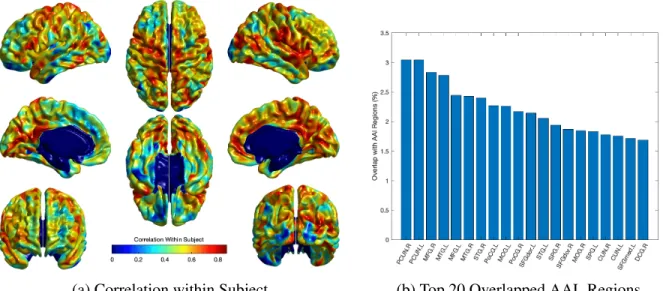
3.9 The correlation of local extra-axial cerebrospinal fluid within subject across age . . . . 61
3.10 Coefficients of variation for local extra-axial cerebrospinal fluid maps . . . 62
3.12 Local extra-axial cerebrospinal fluid change rates per month . . . 63
3.11 Longitudinal local extra-axial cerebrospinal fluid statistics . . . 64
3.13 Longitudinal age effect on local extra-axial cerebrospinal fluid . . . 65
3.14 Longitudinal sexual dimorphism effect on local extra-axial cerebrospinal fluid . . . 66
3.15 Longitudinal sex and age interaction on local extra-axial cerebrospinal fluid . . . 67
4.1 The previous two-stage autism prediction pipeline . . . 71
4.2 Block diagram of the proposed autism prediction system . . . 72
4.3 Deep learning-based isointense MRI segmentation . . . 76
4.4 The extracted cortical measures from input structural MRI . . . 78
4.5 Different parcellation atlases used for dimensionality reduction . . . 81
4.6 Illustration of the proposed deep learning classifier . . . 83
4.7 Local extra-axial cerebrospinal fluid risk groups statistics . . . 84
4.8 Group effect on local extra-axial cerebrospinal fluid . . . 85
4.9 Group effect on regional extra-axial cerebrospinal fluid . . . 87
4.10 Classifier ensemble used to combine individual classifiers decisions . . . 90
4.11 Distribution of the vote count generated by the classifier ensemble . . . 93
5.1 Deep learning-based framework for disease prediction . . . 97
5.2 Proposed convolutional learning on cortical surfaces . . . 100
5.3 Geodesic paths created using different methods . . . 102
5.5 Resampled surface using repeated edge collapse . . . 105
5.6 The proposed network architecture on cortical surfaces . . . 107
5.7 An alternative to the proposed Surface-CNN architecture on cortical surfaces . . . 108
5.8 Illustration of the distortion introduced by geometry images . . . 110
5.9 Visualization of the class-specific mean learned features . . . 111
5.10 Brain regions with statistically significant group differences . . . 111
5.11 Segmented subcortical structures with corresponding surface Meshes . . . 114
5.12 The proposed network architecture on subcortical surfaces. . . 115
6.1 Image slices and corresponding histograms from different scanners . . . 119
6.2 The proposed multi-modal networks, which utilize new multi-modal blocks . . . 122
6.3 Conventional approaches to performing multi-task learning in deep neural networks 125 6.4 Examples of scan meta-data in the combined ADNI dataset . . . 128
6.5 Steps applied to generate tissue segmentation ground truth labels . . . 129
6.6 Distributions of normalized mean brain tissues . . . 130
6.7 Tissue segmentation networks used to generate baseline results . . . 132
6.9 Examples of scan meta-data in the scans included from ADNI1 dataset . . . 134
6.10 Demographic information of the scans included from ADNI1 dataset . . . 135
6.11 Segmented subcortical structures obtained using the FreeSurfer pipeline . . . 136
7.1 Illustration of the out-of-sample/ anomaly detection problem . . . 140
7.2 Proposed framework for out-of-sample detection . . . 143
7.3 Illustration of one-class support vector machine . . . 148
7.4 Examples from the used four-point quality control scoring system . . . 151
7.5 MRI examples that failed image quality control . . . 152
7.6 Normalized histograms of different out-of-sample scores . . . 156
LIST OF ABBREVIATIONS
ACC Accuracy
AD Alzheimer’s Disease
ADI-R Autism Diagnostic Interview-Revised
ADNI Alzheimer’s Disease Neuroimaging Initiative
ADOS Autism Diagnostic Observation Schedule-G
AEs Autoencoders
AI Artificial Intelligence
ASD Autism Spectrum Disorder
AUC Area Under the ROC Curve
BCP Baby Connectome Project
CN Control
CNNs Convolutional Neural Networks
CSF Cerebrospinal Fluid
CT Cortical Thickness
CV Coefficient of Variation
DNN Deep Neural Network
DSC Dice Similarity Coefficient
EA-CSF Extra-Axial CSF
EBDS Early Brain Development Study
EMD Earth Mover’s Distance
FD Fractal Dimension
FDR False Discovery Rate
FMM Fast Marching Method
FN False Negatives
FP False Positives
GANs Generative Adversarial Networks
GI Gyrification Index
GM Gray Matter
GMM Gaussian Mixture Model
GPUs Graphics Processing Units
HR High-familial Risk
IBIS Infant Brain Imaging Study
ICV Intra-cranial Volume
LR Low-familial Risk
MAE Mean Absolute Error
MLP Multilayer Perceptron
MMSE Mini-Mental State Examination
MRI Magnetic Resonance Imaging
MTL Multi-Task Learning
NDDs Neurodevelopmental Disorders
NPV Negative Predictive Value
OC-SVM one-class SVM
PDE Partial Differential Equation
PPV Positive Predictive Value
PVE Partial Volume Effects
QC Quality Control
ReLU Rectified Linear Unit
SA Surface Area
SCI Shape Complexity Index
SEN Sensitivity
SMC Significant Memory Concern
SMOTE Synthetic Minority Over-sampling
sMRI Structural MRI
SPC Specificity
T1w T1-weighted
T2w T2-weighted
TN True Negatives
TP True Positives
VAEs Variational Autoencoders
VBM Voxel-based Morphometry
CHAPTER 1: INTRODUCTION
1.1 Overview
appearance, considerable age-related intensity changes, and severe partial volume effect due to the small brain size. Since most of the existing tools were designed for adult brain MRI data, infant-specific computational neuroanatomy tools are a relatively recent development.
success is due mostly to the rapid progress in computational power, in particular through Graphics Processing Units (GPUs), which enabled the fast development of complex deep learning algorithms. Several types of deep learning architectures have been developed for different tasks, including object detection, speech recognition, and classification. In turn, the success of deep learning in computer vision leads to its use in medical image analysis: for image segmentation (Akkus et al., 2017), image registration (Yang et al., 2017), image fusion (Suk et al., 2014), lesion detection (Kooi et al., 2017), and computer-aided diagnosis (Hoo-Chang et al., 2016). While deep learning-based methods have made significant strides in medical imaging applications, there are still significant open problems, and relatively few methods have been applied to infant MRI datasets. Therefore, there is still a need to develop deep learning methods that can learn from such complex datasets in a way that tackles open issues including low data size restrictions, class imbalance problems, and lack of interpretation of the resulting deep learning solutions.
There has been a limited effort to utilize deep learning techniques for early prediction of NDDs using complex infant neuroimaging datasets. This dissertation identifies key challenges that need to be tackled when performing such an analysis:
[1] Extracting cost-effective, accurate, and reliable, presymptomatic, local imaging biomarkers for NDDs diagnosis. Deriving disease-specific features is critical for identifying high-risk infants who would benefit from very early intervention.
[2] Determining optimal strategies to learn from a diverse high-dimensional feature space effi-ciently. This includes adopting dimensionality reduction techniques that avoid losing relevant information and identifying a parsimonious subset of features needed for optimal performance.
[4] Improving the robustness of multi-task deep learning models utilizing multi-modal imaging datasets. The ability to predict disease-related dimensional scores in addition to categorical diagnostic outcomes would facilitate the development of targeted interventions. The generaliza-tion performance of such a multi-task learning model can further be improved by leveraging multi-modal datasets (i.e., includes imaging and non-imaging information).
[5] Detecting samples from untrained classes in imbalanced and heterogeneous settings typically encountered when studying NDDs. This challenge can be tackled by formulating the problem as anomaly detection with generative deep learning models trained to recognize samples from the well-represented classes. Such a framework would help improve the robustness of deep learning models, increasing the confidence of the clinical decisions made using such models.
This dissertation describes novel methodological contributions to tackle the challenges above (Figure 1.1). First, I introduce a Laplacian-based method for quantifying a local measure of Cerebrospinal Fluid (CSF) from structural MRI. Next, I describe an approach for combining morphometric cortical measurements for early disease diagnosis. Then, I propose a data-driven approach for extending Convolutional Neural Networks (CNNs) for use on non-Euclidean cortical surfaces. I also present a framework for multi-task learning utilizing multi-modal information to improve the robustness of the learned models. Finally, I propose a generative approach to identify samples from untrained classes in imbalanced and heterogeneous settings.
ROI-Based Learning Chapter 4:
Deep-ASD
Diagnostic Prediction
Anomaly Detection Chapter 7:
Anomaly-VAEGAN
Single-Task Multi-Task
Surface-Based Learning Chapter 5:
Surface-CNN
Multi-Modal Learning Chapter 6:
MM-Net
Data Analysis
Data Acquisition
Data Processing
Chapter 3:
Local EA-CSF Measurements
Quantification
1.2 Motivating Problems and Proposed Solutions
1.2.1 Current Findings on Early Prediction of ASD from Neuroimaging Studies
Motivation: Behavioral symptoms that are characteristic of ASD are generally not evident until the second year of life (Rogers, 2009; Ozonoff et al., 2010; Landa et al., 2013; Zwaigenbaum et al., 2005) and then consolidate into the clinical diagnosis of ASD around 2-3 years of age (Rice, 2009). Observable behavioral markers in the first year have not yet been shown to be sensitive or specific enough for accurate prediction of later ASD diagnosis, with Positive Predictive Value (PPV)s of 50% or lower (Ozonoff et al., 2009; Chawarska et al., 2014; Bussu et al., 2018). The current clinical practice is to initiate treatment only after behavioral symptoms arise in the second year of life, or after diagnosis is made between 2-3 years of age. Early interventions have been shown to be more effective than later interventions (Rogers and Vismara, 2008; Clark et al., 2018; Dawson et al., 2010; Vivanti et al., 2016; Rogers et al., 2014; Green et al., 2015; Jones et al., 2017; Cidav et al., 2017) and treatment in infancy, during the period of maximal postnatal brain plasticity, may be even more efficacious (Green et al., 2015). Thus, there is a strong rationale for identifying early, pre-symptomatic markers of ASD to accurately identify those children at highest risk who may benefit most from the pre-symptomatic intervention for ASD.
at 6 months of age was found in infants who developed ASD two years later (Shen et al., 2013, 2017). Collectively, these previous studies demonstrated that pre-symptomatic brain markers of ASD are present in the first year of life before the full manifestation of the disorder, suggesting that a combination of cortical surface anatomy and CSF volume may be useful in predicting later ASD.
My Contributions: The approaches taken to date had several notable limitations. In the previous report using sMRI (Hazlett et al., 2017) of cortical surface area required predictors at both 6 and 12 months of age; the global measurement of EA-CSF volume lacked sufficient specificity to serve as a single predictor of later diagnosis; and the prediction based on functional connectivity MRI was conducted on a small sample and required acquisition and processing methods that may be more complex to implement for widespread clinical applications. To address these limitations,I first propose a novel framework, calledLocal EA-CSF, for the automatic computation of EA-CSF measurements in a way that is suitable for localized analysis. The proposed processing relies on probabilistic brain tissue segmentation, cortical surface reconstruction, as well as streamline-based quantification to produce local EA-CSF measurements. Then,I propose a new deep learning-based framework, namelyDeep-ASD, with the objective of optimally combining multiple measures of infant brain shape and CSF from a conventional sMRI scan at 6 months to improve the accuracy of predicting ASD diagnosis at 24 months. While an accurate prediction can be clinically relevant: it is also crucially important to provide information on how the prediction is made and how that generates a better understanding of the disease. Hence, the proposed framework additionally aims to identify which input features have the most significant impact on the prediction performance.
1.2.2 Deep Convolutional Learning on Non-Euclidean Cortical Surfaces
finely-sampled 2D cortical surfaces, forming a high-dimensional feature list. Based on the extracted features, machine learning classifiers can be used to predict diagnostic outcomes. Such classifiers undergo a training process in which they learn category labels for each set of features. However, with limited datasets, it is hard to train stable classifiers using such a high-dimensional feature space without overfitting. To solve this problem, a dimensionality reduction step becomes necessary for improving the prediction performance of the predictors, providing faster and more cost-effective predictors and providing a better understanding of the underlying process that generated the data.
Dimensionality reduction can be performed using machine learning techniques in a supervised or unsupervised manner (Van Der Maaten et al., 2009). However, unsupervised methods run the risk of losing relevant information while supervised methods tend to be more biased and therefore harder to generalize. Alternatively, if possible, dimensionality can be reduced by first summarizing the features via prior anatomical knowledge, such as summarizing vertex-wise cortical features via a cortical subdivision that divides the cortex into a mosaic of anatomically and/or functionally distinct, spatially adjacent areas using prior parcellation atlases (Glasser et al., 2016). For example, in the ASD prediction framework proposed in (Hazlett et al., 2017), cortical measurements were first summarized using the Brodmann-based automatic anatomic labeling atlas, namely AAL (Achard et al., 2006; Tzourio-Mazoyer et al., 2002). However, current parcellation atlases are generic and not optimized to the given age or pathology that is studied, running the risk of losing relevant information that can be critical in the classification process. The reliance on parcellation atlases is particularly problematic in infant studies as currently only adult atlases are employed due to the scarcity of infant cortical surface atlases. Hence, there is a need for data-driven classifiers that can directly learn from a high-dimensional feature space without a separate feature reduction step.
the input data has an irregular non-Euclidean structure is still challenging. Challenges include the missing notion of a grid on a non-Euclidean surface and the additional need for localized kernel design. To solve this problem a generalization of the CNN paradigm to non-Euclidean manifolds was introduced based on a local geodesic system of polar coordinates to extract ”patches,” which are then passed through a cascade of filters and linear and non-linear operators (Masci et al., 2015). The coefficients of the filters and linear combination weights are optimization variables that are learned to minimize a task-specific cost function. Although this implementation is promising, it usually fails if the surface mesh is very irregular or if the radius of the geodesic patches is large compared to a curvature radius of the shape. To solve these drawbacks, one would need to generate highly uniform surface representations as well as to decrease the geodesic path radius, which in turn might be a problem in terms of expected computational complexity. An alternative generalization based on localized frequency analysis (a generalization of the windowed Fourier transform to manifolds) that is used to extract the local behavior of some dense intrinsic descriptor, roughly acting as an analogy to patches in images (Boscaini et al., 2015). The resulting local frequency representations are then passed through a bank of filters whose coefficients are determined by a learning procedure minimizing a task-specific cost. Such implementation addressed some of the limitations described in the previous work; however, this work was only designed to capture shape descriptors on the surface and is not suitable to be used with other surface measures.
1.2.3 Deep Multi-Modal Multi-Task Learning for Robust Representation Learning
incorporate non-imaging information in the network. In the field of medical imaging, a lot of rele-vant non-imaging information is often available; examples of that include patient information (e.g., demographic information, medical history, symptoms), scanner information (e.g., scanner model, field of strength), and acquisition parameters (field of view, image resolution, sequence parameters). The availability of such information to the network might improve the overall performance and robustness by forcing the network to learn parameters that would work in different settings.
keep the models’ parameters similar. Despite the reduced model flexibility, a hard sharing strategy is more commonly used since it forces the network to rely on generalized representations which reduce the chance of overfitting (Baxter, 1997). Another issue to consider when applying MTL is the possibility of learning imbalances in training as some tasks may dominate others during training (Guo et al., 2018). Hence, choosing an appropriate loss or prioritization strategy becomes a necessity. Instead of using a fixed weighted loss function with weights determined through an expensive hyperparameters tuning, automatic methods are being proposed to weight each task loss dynamically. Criteria for dynamically weighting each task loss include using homoscedastic uncertainty (Kendall et al., 2018), task gradient magnitudes (Chen et al., 2017), or running averages of tasks losses (Liu et al., 2019). Alternative approaches include modeling the multi-task problem as a multi-objective problem (Sener and Koltun, 2018); however, such a strategy is still challenged by the need for defining task heuristics or require complex optimization techniques.
My Contributions: To address some of the limitations mentioned above,I propose a novel multi-task multi-modal deep learning framework, namelyMM-Net, which extends a DenseU-Net architecture (Huang et al., 2017) to the simultaneous learning of classification, regression, and segmentation tasks in multi-modal neuroimaging datasets.The proposed architecture relies on novel multi-modal convolutional blocks to combine imaging and non-imaging information effectively at each level of the network. In addition to a convolutional layer, a multi-modal convolutional block also includes a normalization layer, a linear layer, and a nonlinearity to allow efficient information to flow between imaging and non-imaging data. The proposed framework is applied for predicting diagnostic outcomes as well as continuous scores in a disease-related domain from input MRI and associated non-imaging information (e.g., patient demographic data). Moreover, MRI segmentation is also defined as an auxiliary task to improve the performance of main prediction tasks.
1.2.4 Deep Generative Models for Anomaly Detection in Heterogeneous Datasets
However, on problems that involve learning from noisy datasets with highly imbalanced classes, their success is limited (Litjens et al., 2017). This problem is exacerbated when developing diagnostic or predictive approaches for infants with NDDs as prevalence rates are commonly low in NDDs (e.g. in ASD,≤2%for the general population and≤20%for high-risk population). It has been recognized that the class imbalance problem has a substantial negative impact on training deep learning models. With imbalanced datasets, deep learning models tend to focus on learning the classes with a large number of examples, leading to poor performance for the classes with a small number of examples. In a diagnostic setting based on medical image data, misclassification costs are typically unequal and classifying a diseased sample (minority class) as typical (majority class) has significant consequences that should be avoided. Currently there is no consensus on the effects of the class imbalance issues and how to mitigate this problem optimally; this limitation could affect the reproducibility and accuracy of medical imaging research.
Prior Work:Several medical imaging out-of-sample methods have been proposed that utilize deep generative architectures such as Variational Autoencoders (VAEs) or Generative Adversarial Networks (GANs). VAEs explicitly try to approximate the data distribution of the training data both in the latent and the original space by maximizing a variational lower bound (Kingma and Welling, 2013). In the original space, out-of-sample detection can be performed using the reconstruction score (Lu and Xu, 2018) or distance- or density-based approaches (Vasilev et al., 2018). Anomalies can also be detected in the learned latent space using VAE regularizer scores (Lu and Xu, 2018) or an offline one-class support vector machines (El Azami et al., 2016). Compared to VAEs, GANs avoid any strong distributional assumptions by implicitly specifying probabilistic models describing a stochastic procedure to generate higher quality images directly (Goodfellow et al., 2014). GAN-based anomaly detection for testing samples is performed based on post hoc estimated likelihood scores (Schlegl et al., 2017). Nonetheless, GANs are still challenging to train, and the post hoc score estimators are very slow and tend to produce inaccurate likelihood estimates. In 2018, architectures utilizing both VAE and GAN were introduced for pixel-wise anomaly detection. Chen and Konukoglu (Chen and Konukoglu, 2018) used an adversarial autoencoder (Makhzani et al., 2015) with latent space consistency constraints to identify anomalies based on created reconstruction error maps. Similarly, an architecture that combines a VAE and a GAN was also proposed (Baur et al., 2018) to detect within image anomalies, which showed improvements over the GAN-only approach in (Schlegl et al., 2017). However, these models were designed to detect only pixel-wise anomalies in limited 2D homogeneous datasets and failed to incorporate external information to organize the learned image manifolds. Hence, there is still a need for a new architecture to provide sample-wise anomaly scores in 3D high-dimensional heterogeneous data.
generated images. The encoded latent representations were constrained according to user-defined properties through a jointly trained predictor network. Anomalous samples are detected using learned similarity scores and/or scores from an online one-class neural network.
1.3 Thesis Statement
Thesis: Applied to complex neuroimaging datasets, deep learning models can obtain an ac-curate and robust prediction of neurodevelopmental disorders and neurodegenerative diseases. However, key issues need to be considered for optimal performance, including (1) extracting relevant imaging and surface features based on prior domain knowledge, (2) determining the optimal parsi-monious subset of cortical surface and imaging features needed for an accurate disease diagnosis, (3) learning from high-dimensional feature space on curved manifolds, (4) modeling modality and task heterogeneities for improved model robustness, and (5) identifying out-of-distribution samples to increase the confidence in the model decisions.
The contributions of this dissertation include
[1] Alocal measure of extra-axial cerebrospinal fluid: a novel framework for the extraction of accurate and reliable local extra-axial cerebrospinal fluid measurements. The proposed software tool is the first to address the problem of quantifying extra-axial cerebrospinal fluid in a way that is suitable for localized surface-based analysis. The proposed tool allows neuroimaging labs to investigate the use of local extra-axial cerebrospinal fluid in early diagnostics of neurodevelopmental disorders and neurodegenerative diseases.
clinically-useful measure for the pre-symptomatic detection of autism, which will enable pre-symptomatic intervention, leading to earlier and more effective treatments for autism.
[3] Aconvolutional neural networks extension to non-Euclidean cortical surfaces:a novel general-ization of convolutional neural networks on non-Euclidean manifolds such as cortical surfaces. A general definition of kernels on cortical surfaces is provided using a locally constructed geodesic grid. An accurate classification in a high-dimensional feature space without the need for a separate dimensionality reduction step is achieved using a learning framework that relies on novel surface convolution, pooling, and resampling layers. The data-driven approach allows the identification of disease phenotypes by providing interpretations of the trained models.
[4] A multi-modal multi-task deep learning architecture for joint representation learning: a novel deep learning architecture for addressing modality and task heterogeneities to improve the robustness of learned models. The proposed architecture relies on novel multi-modal convolutional blocks to combine imaging and non-imaging information effectively at each level of the network. In addition to a convolutional layer, a multi-modal convolutional block also includes a normalization layer, a linear layer, and a nonlinearity to allow information to flow between imaging and non-imaging data. The proposed multi-task learning framework allows for the simultaneous learning of classification, regression, and segmentation tasks defined as a primary or an auxiliary task. In a diagnostic setting the proposed framework allows for the simultaneous prediction of diagnostic outcomes as well as continuous scores in disease-related domains, thereby facilitating the development of targeted, individualized interventions.
semi-supervised discriminator is proposed to stabilize network training and ensure a meaningful learned similarity metric. The encoded latent representations are also constrained using user-defined properties through a jointly trained predictor network.
1.4 Overview of Chapters
CHAPTER 2: BACKGROUND
This chapter presents the background materials required for this dissertation. Section 2.1 highlights the current role of deep learning at each step of a typical neuroimaging processing and analysis pipeline, and discuss the current open challenges utilizing deep learning in infant MRI. Section 2.2 provides an overview of popular cortical surface reconstruction methods and describes different geometric and shape properties extracted from cortical surfaces. Finally, section 2.3 discusses discriminative and generative approaches to deep learning and summarizes the deep learning architectures that are utilized in this dissertation.
2.1 Overview of Deep Learning in Structural MRI Processing and Analysis
MRI Processing and Analysis Pipeline: MRI allows the non-invasive acquisition of 3D images at high spatial resolution. sMRI provides the so-called anatomical images on which one can observe the different tissues that constitute the brain (see Figure 2.1). In addition to T1w MRI to create precise anatomical images, other modalities of images can be acquired utilizing alternative properties of the MR signal (e.g., T2w and T2*w). Currently, T1w and T2w sequences form the
0-month 3-month 6-month 12-month 24-month
Figure 2.2: T1-weighted brain images of a typically-developing infant, scanned longitudinally at 0, 3, 6, 12, and 24 months of age. Longitudinal MRI scans allow researchers to study the first year of life, leading to critical insights into many neurodevelopmental and neuropsychiatric disorders.
establishment, surface parcellation, and extraction of surface-based features (Fischl, 2012; Ad-Dabbagh et al., 2006; Styner et al., 2006).(3)Feature preprocessing, feature extraction, machine learning model training, and prediction of unseen subjects (Kim et al., 2016b; Mostapha et al., 2018b; Kim et al., 2005; Hazlett et al., 2017).
Image Preprocessing
Tissue Segmentation
Regional Labeling
Volume-based Measurements
Surface Reconstruction
Surface Correspondence
Surface Parcellation
Surface-based Measurements
Infant sMRI Brain Images
Non-Imaging Information
Training Dataset Testing Dataset
Cortical Measurements Volumetric
Measurements Image
Intensities Demographic
Information
. Age
Sex.
Labeled Data Unlabeled Data
Training of a Machine Learning Model Labels Prediction for New Subjects Complex Neuroimaging
Dataset
Figure 2.4: Venn diagram illustrating the re-lationship between deep learning, machine learning and artificial intelligence.
learning from complex MRI datasets (LeCun et al., 2015). Alternatively, deep learning (LeCun et al., 2015; Schmidhuber, 2015) overcomes limitations of classical machine learning by directly learning useful representations and features in a data-driven manner (i.e., feature learning).
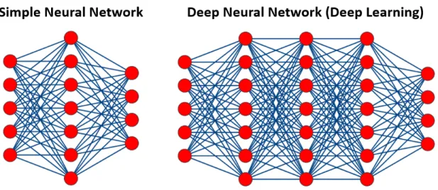
Deep Learning Role: Deep learning refers to advancement in machine learning that is based on the architecture of Artificial Neural Networks. When the number of hidden layers in a neural network is extended, it becomes a Deep Neural Network (DNN) (see Figure 2.5). DNNs allow for the extraction of a complex hierarchy of features from input data while simultaneously performing a task, leading to impressive performance and generalizability (Goodfellow et al., 2016).
Figure 2.5: Architectures of two feed-forward fully-connected neural networks. A classical neural network containing one hidden layer and a deep neural network (deep learning) that has two or more hidden layers. Modern deep neural networks can be based on tens to hundreds of hidden layers.
down-stream applications including image registration (Balakrishnan et al., 2018; de Vos et al., 2019), image segmentation (Dora et al., 2017; Akkus et al., 2017), image retrieval (Qayyum et al., 2017; Pizarro et al., 2019), and disease prediction (Liu et al., 2018; Lu et al., 2018).
While deep learning-based methods have made significant strides in medical imaging appli-cations, there are relatively few methods have been applied in infant MRI data (Mostapha and Styner, 2019). Deep learning methods, designed specifically for infant MRI, were applied in the segmentation of neonatal brain (≤ 1 month) (Moeskops et al., 2016a; Rajchl et al., 2017), the segmentation of isointense infant brain (≈6 months) (Zhang et al., 2015; Moeskops et al., 2016a;
Nie et al., 2016; Moeskops and Pluim, 2017; Huang et al., 2017; Zeng and Zheng, 2018; Nie et al., 2018), and the early detection of NDDs such as ASD (Hazlett et al., 2017).
Current Open Challenges: With recent development in the field of deep learning, many innovative methods have been proposed to improve infant MRI brain image processing and analysis as presented above. The success of deep learning is attributed to its ability to discover general morphological and textural features in a data-driven way. Therefore, deep learning can handle different variabilities in infant MRI brain images that stem from complex brain anatomy and tissue appearance, imaging acquisition protocols, and pathological heterogeneity. However, there are still open issues to address, including the technical challenge of handling 3D medical images, with their added memory and computational consumption requirements. Current approaches to deal with this problem (treating 3D data as stacks of 2D images, patch-based training, and inference, or downsampling 3D images) are not ideal and come with the expense of performance degradation. In infant MRI, other critical challenges arise related to data size, class imbalance, and interpretability, as briefly discussed below.
labeled data imposes additional challenges that need to be addressed. Currently, there has been an effort to make data available through public research data repositories (e.g., NDAR for ASD research), which will allow deep learning models to discover more generalized features in NDDs. To avoid the challenge of training deep learning models from scratch in the context of limited datasets, an alternative is to fine-tune a deep learning model using a technique referred to as transfer learning (Tajbakhsh et al., 2016). For example, a deep learning model can be pretrained using a large dataset of labeled natural images (e.g., ImageNet (Russakovsky et al., 2015)). Nevertheless, it is still challenging to effectively utilize such 2D pre-trained networks for 3D infant MRI applications as such an approach would ignore the anatomical context in directions orthogonal to the 2D plane (Dolz et al., 2018; Xu et al., 2017). On the one hand, training data can be augmented by applying random transformations to the original data (Perez and Wang, 2017). Data augmentation aids in increasing the effective size of training samples and hence reduce overfitting by presenting random variations to the original data during training (Pereira et al., 2016; Akkus et al., 2016). However, augmenting infant MRI datasets is still challenging due to the regionally-heterogeneous image appearance and significant age-related intensity changes. In the presence of NDDs, additional sources of anatomical variabilities are introduced due to the heterogeneous nature of such disorders.
implies significant consequences that should be avoided. Current methods for addressing class imbalance can be classified into those that operate on a training set by altering its class distribution, those that work on the classifier or algorithmic level while keeping the training dataset unchanged, and hybrid methods that that combine the two previously described categories. On the data level, methods which are commonly used in deep learning are based on oversampling, including techniques such as random minority oversampling (Janowczyk and Madabhushi, 2016), Synthetic Minority Over-sampling (SMOTE) (Chawla et al., 2002), and Local Synthetic Instances (Brown et al., 2015). Alternatively, undersampling can be used to solve the class imbalance problem by randomly removing samples from majority classes (Haixiang et al., 2017). In infant MRI, this motivated the development of undersampling methods that only remove redundant examples (Huang et al., 2016). One-class learning is an algorithmic strategy to achieve class balance by training deep learning models to recognize positive samples instead of discriminating between classes (Wang et al., 2015). Finally, hybrid approaches that combine multiple techniques from the previously described methods have been proposed to solve the class imbalance problem (Chawla et al., 2003; Havaei et al., 2017).
nature and hence require subject-specific interpretations. Several techniques were proposed to provide sample-specific interpretation, including the visualization of saliency maps for a given image (Simonyan et al., 2013), scores based on differences at the network output (Shrikumar et al., 2017), and pixel-wise importance estimated using sensitivity analysis (Zintgraf et al., 2017). Another class of methods try to understand individual decisions made by the classifier while assuming a black-box classifier or assuming a particular structure of how decisions are made (Ribeiro et al., 2016; Kumar et al., 2017). Similar methods were designed specifically for understanding CNNs through visualizing feature activity in intermediate layers (Zeiler et al., 2011; Shrikumar et al., 2017). The interpretation methods described above can produce valuable insights into what infant predictive deep learning models have learned; however, there is little agreement on how these methods should be evaluated for benchmarking. Interpretability can be evaluated in the context of a given application or using a proxy to provide a quantifiable evaluation (Doshi-Velez and Kim, 2017).
2.2 Cortical Surface Reconstruction and Shape Analysis
2.2.1 Cortical Surface Reconstruction
of designing general energy functions (without heuristics) that can attract the deformable model through the narrow opening of the sulci (Fischl, 2012).
Current Pipelines:Alternatively, current frameworks for cortical surface reconstruction, such as FreeSurfer (Dale et al., 1999) or CIVET (MacDonald et al., 2000) pipelines, identify the White Matter (WM) and GM boundary to aid in reconstructing the surface model. Both the FreeSurfer and CIVET pipelines share the similarity of guaranteeing a spherical topology for the reconstructed WM surface model. Furthermore, the GM surface is obtained by deforming the WM surface to fit the GM and CSF boundary, and consequently, a correspondence between the WM and GM surfaces is naturally established. In summary, the main steps involved in the overall surface reconstruction pipeline are as follows. (1)The intensities of the input MR images are first adjusted via bias field correction and intensity normalization.(2)The preprocessed images are then aligned to a common coordinate space (e.g., Talairach or MNI) for skull stripping and cortical structure segmentation. (3) A WM mask is generated by filling in the subcortical structures within the WM and then separating the results into left and right hemispheres. (4)An initial WM surface is obtained either using a rough triangulated tessellation (FreeSurfer and new versions of CIVET) or by deforming a topologically correct spherical model (old versions of CIVET).(5)The GM surface is reconstructed by deforming the constructed WM surface through an energy minimization procedure that involves using image intensity information and geometric constraints (e.g., curvature smoothing).
employ infant-specific steps are highly desirable. Recent efforts have been made toward that goal (Li et al., 2015; Kim et al., 2016a); however, publicly available tools are still missing.
T1w
T2w
Tissue Segmentation
6 months 12 months 24 months
White Matter Surface
Gray Matter Surface
2.2.2 Differential Geometry on Surfaces
Since this dissertation involves learning from surface properties extracted from 3D cortical surfaces, I briefly overview the basic concept of differential geometry on 2D manifolds.
X(u,v)
N
T T k r = 1
x
Xu
Xv
T
Tangent Plane Normal Section
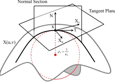
Figure 2.7: Illustration of the definition of the normal curvature on a smooth surface.
Curvature Metrics: LetS ∈R3be a smooth surface with parametrizationX(u, v)∈Ssuch
that the partial derivatives Xu and Xv are linearly independent, where (u, v) ∈ R2. Let T be
the tangent direction at a given pointxonS; the normal curvatureκT atxis a real number that
measures howS bends in the directionT as measured by the swing of the surface normalN atx. The normal curvature is easy to understand as it describes the curvature of the plane curve formed by the intersection ofS with the plane passing throughT, meetingS perpendicularly (Figure 2.7). LetDT be the directional derivative in theT direction. The normal swingDTN atxalongT can
be decomposed into the normal curvatureκT and its geodesic torsionτT according to
DTN =κT ·T +τT ·T⊥, (2.1)
whereT⊥is the perpendicular direction toT in the tangent plane and
Similarly, walking alongT⊥, the normal swing atxin that direction can be expressed as
DT⊥N =κT⊥·T⊥+τT⊥·T. (2.3)
Equations 2.1 and 2.3 can be expressed in matrix form as follows
II=
DTN
DT⊥N
=
κT τT
κT⊥ τT⊥
T T⊥
. (2.4)
The symmetric2×2matrix shown in Equation 2.4 is called the second fundamental form ofS and is denoted by the Roman numeral II. The eigenvalues of II provides what is called the principal curvaturesκ1andκ2, which captures the pure normal swing along the eigenvectors with no geodesic
torsion (i.e.,τ = 0). The general shape morphology of a surface patch is determined by the different sign combinations ofκ1 andκ2, while the magnitude ofκ1andκ2 describes how bent the surface
is irrespective of shape morphology. Hence, each principal curvature separately does not provide a complete interpretation of local surface shape (Koenderink and Van Doorn, 1992). Therefore, to better describe shape proprieties, different geometric properties are described in terms of the principal curvatures(κ1 > κ2), namely mean curvatureH, Gaussian curvatureK, shape indexS,
and curvednessC (Koenderink and Van Doorn, 1992).
H = 1
2(κ1+κ2), K =κ1·κ2
C=−2 πtan
−1
κ1+κ2
−κ1+κ2
, S = 2 πlog
r κ2
1+κ22 2
! (2.5)
Mean Curvature(H)
Gaussian Curvature(K)
Curvedness(C)
Shape Index(S)
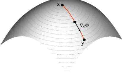
Geodesics and Short Distance Path: Intrinsic distances on a surface S in 3D space is a critical geometric measure for understanding complex shapes. Such distances are computed along geodesics, which are a generalization of the concept of straight lines to a more general setting. Geodesics are also crucial because the shortest path between two points onS always follows a geodesic path, and the shortest distance between two points onSis called a geodesic distance.
Figure 2.9: Illustration of geodesics and shortest path on a smooth surface.
More formally, a geodesic on a smooth surfaceSis a differentiable curve that has zero geodesic curvatureκg at each point on the curve. The geodesic curvature at ax is given byκg = κsinθ,
whereκis curve curvature atx, andθis the angle between surface normalN and the normal to the curven. For a surface and curve embedded inR3, this is equal to describing the geodesic curvature
as the covariant derivative of the tangent vector to the curve (Balasubramanian et al., 2008). It can also be shown that the geodesic distance to a collection of seed points onSsatisfies a non-linear differential equation, called the Eikonal equation (Kimmel and Sethian, 1998b), which is given by
k∇SΦk=F. (2.6)
to the set of seeds. Locally, geodesics are shortest paths since any perturbation of a geodesic curve will increase its length. Hence, the shortest distance between two pointsx, yon the surface are the minimal geodesics connecting those points. As shown in Figure 2.9, a geodesic path connecting xtoy can be computed from the geodesic distance mapΦto one of the points by performing a gradient descent optimization onΦ.
2.2.3 Cortical Surface Proprieties
Thickness Gray Matter
Surface
White Matter Surface Surface Area
Volume
(a) Cortical Thickness, Surface Area, and Volume
(b) Cortical Layers
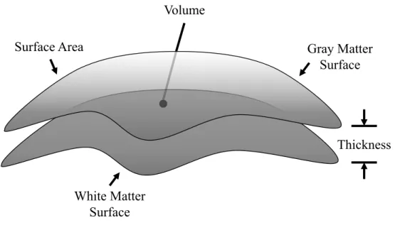
Overview: The cerebral cortex refers to the outer layer of the gray matter, which is a highly folded structure with the degree of folding related to an evolutionary necessity to increase sur-face area without increasing the intracranial size (Magnotta et al., 1999). The cerebral cortex plays a critical role in cognitive development and decline, and alterations in cortical volume have been associated with NDDs (Ismail et al., 2016; Mensen et al., 2017) and neurodegenerative dis-eases (Dickerson et al., 2008). As shown in Figure 2.10, the components of cortical volume, namely Cortical Thickness (CT) and Surface Area (SA), have separable developmental trajectories and are related to distinct neurobiological processes. Though cortical volume measurements are affected by both CT and SA, volume was shown to be more closely linked to SA than CT (Winkler et al., 2010). Hence, in imaging studies conducting surface-based analysis, local measurements of SA and CT need to be examined separately and are preferred over gray matter volumes. Meanwhile, an improved understanding of the factors that dictate the folding of the cerebral cortex is required, as irregular folding patterns observed in individuals affected by NDDs emphasize the clinical importance of understanding the folding process.
Additionally, most studies choose to measure SA at the middle surface, as it captures a combination of both WM and GM surface properties, which is preferred to analyzing both of them separately.
Cortical Thickness: In the absence of a unique definition of a CT measure, several surface-based methods for measuring CT from MRI brain data have been proposed (Wagstyl and Lerch, 2018). Most of the existing methods define the WM surface as the inner surface and the GM as the outer surface. Hence, current methods for measuring CT are sensitive to the quality of the provided tissue segmentation (i.e., WM/GM and GM/CSF boundaries), leading to uncertainties in the obtained measurements due to loss of available information (Aganj et al., 2009). Following the construction of inner and outer surfaces, methods differ in their approach to computing the required thickness measure. Coupled surface methods (Fischl and Dale, 2000; MacDonald et al., 2000) employ the Euclidean distance between corresponding points on the inner and outer surfaces as the CT measure, which may lead to an overestimation of the thickness. To mitigate this, closest point methods (Miller et al., 2000) would first find for each point on the inner or outer surface, the closest point on the other surface and then would compute the Euclidean distance between them. To tackle the absence of symmetry in closest point-based CT measurements, methods that solve Laplace’s equation in the GM region was proposed (Yezzi and Prince, 2003; Haidar and Soul, 2006). In these methods constant, but opposite-in-sign boundary condition potentials are set on each of the two surfaces. The CT is then defined as the length of the streamline obtained by tracing the gradient of the resultant vector field, which leads to a uniquely assigned measure at every point. Compared to coupled surface and closet point methods that utilize straight-line distances, streamline based CT leads to biologically meaningful measure as it captures the curved nature of cortical layers. Studies conducted to validate current CT methods on simulated data (LERCH et al., 2003) indicated significant differences among different cortical thickness metrics and emphasized the critical importance of an appropriate smoothing of obtained CT measures for optimal results.
of cortical gyrification (Toro and Burnod, 2005), which offers insights to understand abnormal cortical folding in brain disorders (Van Essen et al., 2006). Over the years different methods have been proposed to quantify cortical folding during early brain development. Methods utilizing local geometric features (e.g., curvature information) have been proposed to quantify cortical folding at a local scale or a more global scale by integrating such features across different brain regions or an entire hemisphere. Some of these methods provide measures that depend on the cortical surface area (Ajayi-Obe et al., 2000; Van Essen and Drury, 1997); this dependence limits their usefulness in developmental studies with brain size variations associated with gestational age and between different NDDs populations. Alternately, measures of global curvature that are independent of surface area have also been proposed to study cortical folding in early brain development (Rodriguez-Carranza et al., 2008; Awate et al., 2010). However, such measures still were unable to distinguish between normal and aberrant cortical development (Shimony et al., 2016).
areas that may be functionally quite different. To tackle this issue, local GI measures that utilize spatially varying kernels that encode cortical folding patterns were proposed (Lyu et al., 2018).
Another fine-scale measurement of cortical surface complexity, referred to as the Shape Com-plexity Index (SCI) (Kim et al., 2016b), was proposed as an alternative to quantifying cortical folding. In contrast to the local GI, the SCI can detect whether a sulcal or gyral region experiences a widening or deepening process as well as capture the development of secondary and tertiary sulci. As shown in Figure 2.11, the shape indexSis first calculated at each point on the surface, which yields a score ranging from -1 to 1. TheS score is then dichotomized into predefined different geometric, topological situations. The SCI score is then assigned to reflect theS variability within a local region, measured from theS histogram within a given geodesic distance. Particularly, the discrete Earth Mover’s Distance (EMD) is used to compute the difference between the observed S distribution and each of the defined basic topological settings; then the minimal EMD at each point is used as a measure of surface complexity. This results in an SCI score that ranges from 0 to 1 since the minimum EMD is maximally 1 over the selected geometric settings (the observed distribution is balanced and bi-modal at theSextrema of 1 and -1).
SCI = 0.9545
2.3 Common Deep Learning Architectures
In this section, I briefly overview discriminative and generative deep learning architectures that are being utilized in this dissertation to effectively learn from input complex neuroimaging datasets.
Discriminative and Generative Deep Learning:The key to the success of machine learning models rests in their ability to extract high-level and semantically meaningful features from the complex neuroimaging datasets. As shown in Figure 2.12, two main approaches have been proposed to achieve that goal, namely learning using discriminative models or generative models. Supervised learning using discriminative models attempts to directly learn the posterior,p(y|x), of the inputs x and the label y, or learn a direct map from inputsxto the class labelsy. The intution behind these models is that a good performance on the given supervised task must indicate that useful and meaningful high-level features have been learned.
Figure 2.12: Illustration of generative vs. discriminative learning approaches. Discriminative models focus on classification boundaries between different classes, whereas generative models emphasize the data generation process in each particular class.
generative learning seeks to model the input data,p(x), without expecting the availability of training labels. In a supervised setting, generative models can also be trained to learn a model of the joint probability,p(x, y), where predictions can be made by first computingp(y|x)using Bayes rule and by then picking the most likely labely(Ng and Jordan, 2002). With generative learning, the intuition is that if the model can efficiently and faithfully generate the data, then a good latent representation must have been learned. Generative models are promising in providing solutions for problems associated with learning from complex neuroimaging datasets; however, such models are challenged by high-dimensional data with complicated data manifolds. Below, deep discriminative (e.g., MLP, CNN, U-Net, DenseNet) and generative (e.g., VAE, GAN) architectures are reviewed. Multilayer Perceptron: A neural network that has at least one hidden layer and all layers are fully-connected is referred to as a Multilayer Perceptron (MLP) (see Figure 2.5). MLPs is a fundamental tool that provides the foundation of many advanced techniques in deep learning. Mathematically, an MLP is a composite function of alternating affine and non-linear transformations, which can be expressed as
f(x) = g(Wlφl−1(Wl−1(· · ·φ1(W1x+b1)· · ·+bl−1) +bl), (2.7)
whereWi,bi,φiare theith layer’s weights, biases, and activation function respectively andg is the
Convolutional Neural Networks for Classification Tasks: Unlike MLPs, where inputs are always in vector form, CNNs maintain and utilize the structural and spatial information among neighboring pixels or voxels in the input 2D or 3D images. Also, as illustrated in Figure 2.13, CNNs limit the degrees of freedom of the deep learning model through exploiting a local receptive field, weights sharing, and sub-sampling techniques. Hence, this will result in models that can learn from limited datasets usually present in medical applications in a way that is less prone to overfitting.
Figure 2.13: Illustration of how convolutional neural networks control the model complexity through three fundamental mechanisms, namely, local receptive field, weight sharing, and subsampling.
Figure 2.14: AlexNet, a convolutional neural network designed by Alex Krizhevsky (Krizhevsky et al., 2012). it achieves a 10.8% better error performance than the runner up in the 2012 ImageNet competition that used a shallow machine learning method. AlexNet has eight layers; the first five were convolutional layers, max-pooling layers follow some of these, and the last three layers were fully connected. AlexNet was written with CUDA to be trained using GPUs, which made the computationally expensive training of such a complex network feasible.
1. Convolutional Layer: A convolutional layer is designed to detect localized features extracted at different locations in the input feature maps using learnable kernels or filters. Notably, the inputI to the convolutional layer is convolved with a set of small parameterized filters, also called kernelsK. In practice, most deep learning libraries utilize cross-correlation is instead of the convolution operation (cross-correlation does not ”flip” the kernel). Hence, the output at i, j, k voxel coordinates produced by a 3D convolution can be written as
(I∗K)(i, j, k) =
m
X
1
n
X
1
p
X
1
I(i+m, j +n, k+p)K(m, n, p), (2.8)
model,(3)padding type, which controls how convolution is performed on the borders of the input, and(4)stride value, which controls the step of the convolution filter.
2. Activation Layer: The output of convolutional layers is passed through non-linearities in-troduced by an activation function. This makes it possible for the entire neural network to approximate almost any nonlinear function similar to an MLP. The Rectified Linear Unit (ReLU), defined as ReLU(x) = max(0, x), and its alterations, such as Leaky ReLU or para-metric ReLUs, are among the most commonly used activation functions (Clevert et al., 2015). These functions enabled the training of deeper models in a way that avoids vanishing gradient problems typically found when using the more traditional tanh and sigmoid activation functions.
3. Pooling Layer: Feature maps produced by feeding the data through convolutional and activation layers are then typically downsampled or pooled using a pooling layer. Pooling operations are applied to small grid regions to produce a single number summary for each region. This summary measure can be computed by using the max function (max-pooling) or the average function (average pooling). As a small shift of the input image would result in insignificant alterations to the activation maps, pooling layers provide CNNs with translational invariance. Recently, strided convolutions are more commonly used as an alternative to achieve the required downsampling. Such approach simplifies the network by removing pooling layers while maintaining similar performance levels (Springenberg et al., 2014).
4. Dropout Layer: In addition to the commonly used`1 and`2 losses as regularization techniques
5. Batch Normalization Layer:These layers are placed after activation layers, providing normal-ized activation maps by first subtracting the meanµand dividing by the standard deviationσ for each training batch, followed by a learnable scaleγ and shiftβ(Ioffe and Szegedy, 2015):
ˆ
x= √x−µ σ2+
y =γ·xˆ+β
(2.9)
By forcing the network to periodically standardize activation maps as the training batch runs through batch normalization layers, the network becomes better regularized, and the training gets simpler leading to faster convergence (Ioffe and Szegedy, 2015). Note that in modern DNNs, in addition to batch normalization, other normalization methods have been proposed such as weight normalization (Salimans and Kingma, 2016), instance normalization(Ulyanov et al., 2016), layer normalization (Ba et al., 2016), and group normalization (Wu and He, 2018).
and pooling layers and include a decoder network that upsamples the higher-level features extracted by the encoder network using deconvolution layers. This produces pixel-wise class probabilities that can be used to classify pixels and produce the required segmentation map.
Figure 2.15: An example of encoder-decoder architecture based on a fully convolutional network that was used to for single modality infant MRI tissue segmentation (Nie et al., 2016).
becomes independent of the number of pooling layers. Similar to a U-Net, information is passed by means of a standard skip connection between the downsampling and the upsampling paths.
Figure 2.16: The U-Net architecture proposed for biomedical image segmentation tasks. The U-Net architecture formed of a contracting path to capture context through compact representations and an expanding path that allows accurate localization, which enables learning from few examples and yields superior segmentation results. Image adapted from (Ronneberger et al., 2015)
Variational Autoencoders: As shown in Figure 2.18a, Autoencoders (AEs) are neural net-works used for unsupervised representation learning. An AE is composed of two netnet-works, an encoder networkEwhich is parametrized byθ and a decoder networkDwith parametersφ; the first network encodes the inputxinto a low-dimensional encoding (latent) spacez, while the second network takes z as its input with the purpose of reconstructing the input xˆ. By restricting the dimensionality of the encodingz, the AE is forced to learn efficient representations of the inputs. Such a model is trained by minimizing a reconstruction loss`(typically`1 or`2) between the input
xand its reconstructionxˆ. On the other hand, as shown in Figure 2.18b, Variational Autoencoders (VAEs) (Kingma and Welling, 2013) present an alternative formulation of the traditional AEs to provide a probabilistic interpretation of the learned latent space.
𝑥 𝑧 #𝑥
Encoder 𝐸%(𝑧|𝑥)
Decoder 𝐷*(𝑥|𝑧)
(a) Autoencoder
𝑥 "𝑥
Encoder
𝐸$(𝑧|𝑥)
Decoder
𝐷*(𝑥|𝑧) 𝜇,
𝜎,
𝜀~𝑁(0,1)
𝑧 = 𝜇,+ 𝜎, 6 𝜀
(b) Variational Autoencoder
In VAEs, the encoder networkE now outputs two parametersµz andσz used in sampling a
point in the Gaussian distributionN(µz, σz)modeled byE. To find the optimal network parameters
θandφ, a variational lower bound loss`V AE need to be minimized. This involve minimizing the
reconstruction error betweenxandxˆand theKLdivergence term`KL of the distribution modeled
byE and some prior distributionp(z)such as the standard Gaussian distributionN(0, I).
`V AE =`rec+`KL =`(x,xˆ) +KL(N(µz, σz)||p(z)). (2.10)
Directly samplingzfromN(µz, σz)would result in noncomputable gradients which would prevent
backpropagating the error during training. The so-called ”reparameterization trick” is used to solve this problem by moving the sampling operation to the input layer. In particular, ε ∼ N(0,1)is added to the model to make the sampling operation differentiable by multiplying it toσz.
Advantages of using VAEs include that there is a clear and recognized way to evaluate the quality of the model using the estimated log-likelihood (variational lower bound). However, due to the strong assumptions and approximations involved, they may lead to suboptimal models and the generated images tend to be more blurred than those coming from competing generative methods. Generative Adversarial Networks: In contrast to VAEs that explicitly try to approximate the true data distribution, Generative Adversarial Networks (GANs) implicitly specify probabilistic models that describe a stochastic procedure to directly generate data. Such a framework for constructing generative models can provide samples that are sharp and compelling without having to specify a likelihood function. As shown in Figure 2.19, GANs contain two simultaneously trained networks, namely a generator networkGand a discriminator networkDwith parametersθandα respectively. GAN training is based on a game-theoretic scenario, where two players are competing in a zero-sum game. Particularly, the generatorGtask, conditioned on a sampled noise variable z ∼ p(z), is to generate samples that follow the real distribution of the datap(x). On the other
hand, the discriminatorDtries to distinguish between real dataxand the fake generated dataxˆ
by outputting a probability scoreDφ(x)∈[0,1]. In this adversarial arrangement, training is done