4782.pdf

(1)

Addressing the Computational Cost of the Immersed Boundary

Method through Multi-Implicit and Multi-Rate Strategies with

Time Parallelism

Lauren E Fovargue

A dissertation submitted to the faculty of the University of North Carolina at Chapel Hill in partial fulfillment of the requirements for the degree of Doctor of Philosophy in the Department of Mathematics.

Chapel Hill 2012

Approved by:

Michael L Minion

Laura A Miller

Jingfang Huang

Jan F Prins

(2)

Abstract

LAUREN E FOVARGUE: Addressing the Computational Cost of the Immersed Boundary Method through Multi-Implicit and Multi-Rate Strategies with Time

Parallelism

(Under the direction of Michael L Minion)

Many problems in biological fluid-structure interaction have been studied with Pe-skin’simmersed boundary method (IBM). This method defines a relatively simple math-ematical modeling framework, and allows for the use of standard fluid solvers. However, when evaluated computationally in many applications, a very small time step is required. This time step is not restricted by accuracy, but stability, causing the temporal problem to be stiff. Previous attempts to address the stability restriction of IBM use semi or fully implicit schemes that require the code, including the fluid solver, to be rewritten, and these have yet to be implemented in application focused studies.

(3)

ACKNOWLEDGMENTS

I want to thank my wonderful husband Dan for his constant support and reassurance and for building a life with me, without your help, both in math and at home, I wouldn’t have made it to this point. Thank you for being the strongest part of me.

Thank you to Dr. Minion who was a great advisor and mentor, your guidance and help has taken me from a clueless graduate student to a confident novice scientist. Thank you for not giving up on me and pushing me to take my own research by the horns, I can’t express how valuable that will be to my future. Don’t worry, I will continue to push for SDC and have an answer to “you can’t do parallel in time”. Thank you so much for all your time and effort over the last few years, I will always be proud to be one of Minion’s minions.

Thank you to Laura Miller, for being a mentor, travel companion and most of all, friend. Thank you for showing me the beauty of biology, which ignited my interest in it, and being a constant source of encouragement, I couldn’t have done it without you.

Thank you to all my professors here at UNC, especially those who taught computa-tional classes. Dr. Minion, Dr. Miller, Dr. Huang, Dr. Adalsteinsson, and Dr. Mitran. You have inspired a pure math background into a love of numerics and for that I cannot thank you enough.

A big thank you to my window for getting me through my 4th and 5th years and my 4th year office mate Christy Hamlet, who shall always hold the title of office genius. Thank you to Brandyn Lee, my 5th year office mate, whose brilliance is (hopefully) contagious and stories priceless. Thank you to Emily Braley, for being a workout partner,

(4)

(5)

List of Tables

Table 4.1. Coefficients for H1(r) . . . 39

Table 4.2. Coefficients for H2(r) . . . 41

Table 4.3. Optimal coefficients for H1(r), H2(r) on a 128 x 128 grid . . . 44

Table 4.4. Optimal coefficients for H1(r), H2(r) on a 256 x 256 grid . . . 44

Table 4.5. Optimal coefficients for H1(r), H2(r) for δ= 4∆x . . . 44

Table 4.6. Optimal coefficients for H1(r), H2(r) for δ= 4/128 . . . 46

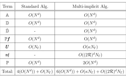
Table 5.1. Operation count for the standard and multi-implicit algorithms. . . 52

Table 6.1. Operation count for the standard and multirate algorithms . . . 69

(8)

List of Figures

1.1. Thysanoptera, or a thrip, is a tiny wasp [47]. . . 2

1.2. Heart with prosthetic mitral valve [35]. . . 3

1.3. Glycocalyx in a rat capillary [75]. . . 3

2.1. The two dimensional FSI problem with domain Ω and immersed fiber Γ . . . 7

2.2. Close up on part of Ω and Γ, discretized in 2D. . . 13

2.3. Springs connecting points on Γ, producing a force,FFF_γ at point XXX_γ . . . 14

2.4. Regularized blob, Bδ(r) . . . 16

3.1. A full time step, [tn, tn+1] with SDC nodes tm . . . 21

3.2. A full time step, [tn, tn+1] with SDC nodes tm and sub-SDC nodes, tp . . . 27

3.3. Number of SDC correction sweeps vs. error, solving (3.34) with different ’s 31 4.1. Scaling of_Pfff and ∇_Pfff with the spring constant k . . . 33

4.2. The two radially symmetric terms of_Pfff, for a fixedδ . . . 34

4.3. Components of the splitting function . . . 36

4.4. H1(r) withR = 1 and labeled matching conditions . . . 37

4.5. H2(r) withR = 1 and labeled matching conditions . . . 38

4.6. H1(r) withR = 1 and matching conditions (i)-(iv), given in Table 4.1 . . . 40

4.7. H2(r) withR = 1 and matching conditions (i)-(iv), given in Table 4.2 . . . 42

4.8. Perturbed Ellipse. . . 42

4.9. Coefficients with 128×128 grid, NΓ = 400 with δ= 4/128, and R = 1 . . . 43

4.10. Coefficiens with 256×256 grid with δ= 4/256, NΓ= 800 and R= 1 . . . 43

4.11. Grid size vs. Ratio of |_Pfff /ff|and |∇_Pfff /∇ff|, δ= 4/128 . . . 45

4.12. Grid size vs. Ratio of |_Pfff /ff|and |∇_Pfff /∇ff|, δ= 4∆x . . . 45

(9)

5.2. Error and computational cost for different values R . . . 54

5.3. Spring force model for the immersed boundary. . . 57

5.4. Depiction of target points attached to half of the immersed boundary. . . 58

5.5. The forced circle, non-stiff test problem . . . 59

5.6. Convergence of the standard and multi-implicit algorithm. . . 61

5.7. The straight wings stiff test problem. . . 62

5.8. Multi-implicit and standard algorithms on the stiff test problem. . . 63

6.1. One time step [tn, tn+ 1] with SDC nodes and sub-SDC nodes . . . 65

6.2. Effect ofR and P on error, with cost, in a non-stiff problem . . . 70

6.3. Convergence of the multirate algorithm on the non-stiff problem . . . 71

6.4. Relative fluid velocity error for the stiff problem with the multirate algorithm. 72 6.5. Fiber position error for the stiff problem with the multirate algorithm. . . 72

6.6. Convergence of the multi-rate, multi-implicit algorithm. . . 75

6.7. Result of using the multi-implicit, multirate algorithm on the stiff problem 75 7.1. Error vs. iteration number for PFASST/BPM . . . 84

7.2. Error vs. time for PFASST/BPM . . . 84

9.1. Screenshots of H1(r) withR= 2 and labeled matching conditions . . . 96

9.4. Screenshots H2(r) withR = 3 and labeled matching conditions . . . 97

9.5. H1(r) withR = 2 and matching conditions (v)-(viii) . . . 98

9.6. H1(r) withR = 3 and matching conditions (ix)-(xii) . . . 98

9.7. H2(r) withR = 2 and matching conditions (v)-(viii) . . . 99

9.8. H2(r) withR = 3 and matching conditions (ix)-(xii) . . . 99

(10)

CHAPTER 1

Introduction

There are two categories of interaction for dynamic systems that involve a viscous incompressible fluid and a flexible, dynamic object, one-way and two-way coupling. A system is considered to have a one-way coupling when the dynamics of the fluid or object are prescribed and unaffected by the others motion. Two way coupling occurs when the motion of the fluid and object are mutually dependent on each other, creating a coupled system of equations that are difficult to extract information from, both analytically and numerically. Here the focus is on two-way coupling, specifically problems of biological fluid-structure interaction (FSI), where an elastic, biological structure interacts with a viscous incompressible fluid.

This introduction aims to motivate this class of problems and provide an overview of a particular framework for modeling such problems. This framework, the immersed boundary method, is a popular method for studying biological FSI problems, however when discretized, it can become very computationally expensive. It has been well docu-mented that the time step of this method for many applications has to be small for the purposes of stability, not accuracy, causing it to be computationally expensive.

(11)

Figure 1.1. Thysanoptera, or a thrip, is a tiny wasp [47].

1.1. Motivation

Although the application of mathematics to biology can be dated back at least to the days of Gregor Mendel (1822-1884), recently there has been a surge in the field of mathematical biology [52]. From biologically inspired design, to cancer research, to improving medical procedures, mathematics and computation have helped advance biological research. Not only does using mathematics answer fundamental questions, aiding the direction of biological research, but it advances the field of mathematics, as new techniques are being developed to tackle such problems [52]. Here, contributions to the field of mathematical biology are made by expanding upon current techniques in computational biological fluid (biofluid) dynamics.

There are many questions in biofluid dynamics, such as ‘how do tiny insects fly?’, ‘what happens in the endothelial surface layer’, and ‘what is the optimal design for a mitral valve replacement?’, and computational techniques have helped to provide some understanding [69, 67, 42].

Consider three examples, shown in Figures 1.1, 1.2, 1.3. In each of these cases, there is a coupled dynamic between a viscous incompressible fluid and an elastic biological structure. The first figure (1.1) shows the thrip, a small wasp believed to achieve lift based on the unique structure and Weis-Fogh, “clap and fling”, motion of its wings [67, 68]. The second figure, Fig. 1.2, shows a schematic of a heart, highlighting a mitral

(12)

Figure 1.2. Heart with prosthetic mitral valve [35].

Figure 1.3. Glycocalyx in a rat capillary [75].

valve prolapse, where the leaflets of the heart fall back into the left atrium. This condition may be treated with an artificial replacement of this valve, the optimal design for which has been studied mathematically [42]. Finally, Figure 1.3 shows the endothelial surface layer, or glycocalyx, in a rat capillary. This hair-like structure lines the lumen, or inner region, of capillaries and is widely believed to be a mechanotransducer, that is, it converts mechanical hemodynamic stress into a chemical response [70].

In each of these three examples, there are thin elastic structures (e.g. the wing on the thrip, the ’strings’ on the mitral valve and the glycocalyx itself) with complicated geometry, interacting with a fluid. Fluid behavior can be categorized by the value of the Reynolds number, a dimensionless ratio of inertial forces to viscous forces. It is defined as

(13)

where u is a characteristic velocity, L is a characteristic length scale, ρ the density of the fluid and µ the dynamic viscosity. This definition allows for dynamic similarity, i.e. flows categorized by the same Reynolds number behave in the same way. For example, when viscous forces are increasingly dominant and inertial forces less noticeable, theRe becomes small. This is sometimes mathematically modeled by using the Stokes equations, which neglect the inertial terms. However, fluid where both viscous and inertial forces cannot be ignored, can be modeled with the Navier-Stokes equations. Applications in this fluid regime are targeted here.

Creating a computational simulation for particular FSI problems may requires many discretization points and high resolution, becoming highly computationally expensive. This overwhelming cost leads to the utilization of simplified studies, without the full complexity of the geometry [59, 70, 68, 67, 69]. Although these studies are a necessary first pass to looking at the underlying biological phenomena, more robust simulations could help to further understanding.

1.2. The Immersed Boundary Model

The immersed boundary method(IBM) is a framework to model and simulate biologi-cal FSI problems that has been used in many applications, from hearts to insects [79, 69]. Its popularity with application studies can be pointed to the ‘simplicity’ of the framework and the ability to the use standard fluid solvers. However, there are well known computa-tional bottlenecks with IBM, as the time step required for numerical stability can be very small. That is, the problem becomes stiff, a term meaning that the time step is restricted not by accuracy but stability. This has inspired semi and fully implicit implementations of IBM, to increase the largest stable time step [85, 61, 74, 50, 58, 15]. Most of these methods, though they may achieve a larger stable time step, are more computationally expensive per time step, resulting in little gain in overall run time. Additionally, to date, there has been virtually no use of these methods in applications, which is likely a result of the work it takes to implement these solutions.

(14)

In the literature, there tends to be a division between those who work on the algo-rithms for IBM and those that apply the IBM framework to get biologically significant results, with some important exceptions [81, 62, 42]. In the case of the latter, there is more emphasis on the biological modeling and results, with less focus on involved computing. Once one has implemented the IB framework, significant changes do not need to be made to study different applications, and in particular no changes need to be made to the fluid solver. Thus it may not be efficient to spend time, for example, implementing a nonlinear solver or preconditioning for a moderate run time reduction. Additionally, many of these semi and fully implicit techniques require an entire rewrite of the IBM code, including the fluid solver, and the time it takes to do so may not be worth it to those interested in application. There does not appear, to date, to be a sufficient approach that can reduce simulation run time and not require great changes to existing IBM code.

1.3. Thesis statement

(15)

Spatial splitting, multi-rate, multi-implicit methods, and time parallelization have been used in other types of stiff problems, and the success of these implementations is what motivated the work presented here. Bouzarth et. al. split the spatial field for FSI problems where viscous forces overpower inertial forces, known as the Stokes regime, and employed multirate methods to increase the efficiency of the method of regularized Stokeslets[8]. Effectively, the work here is an extension of the ideas of Bouzarth, to flow where inertial forces cannot be ignored and the use of IBM, as well as multi-implicit and time parallelism considerations. Other studies, such as Bourlouix et. al. found that using a multi-implicit technique for advection-diffusion-reaction equations yielded a computa-tional advantage when the reaction term was significantly stiffer than the other parts of the equation [7]. Time parallelization with the parallel full approximation scheme in space and time (PFASST) has shown better convergence and lower error, although with-out increased efficiency, in the work of Emmett and Minion, where the Viscous Burgers equation and the Kuramoto-Silvashinky equation were considered [29]. Potenetially, a combination of these methods is promising to reducing computational time while keeping error low. The critical common denominator in all of these works is the use of spectral deferred corrections (SDC), a stable, high order method for time integration. Thus it is employed here as well, and details about this choice and the particular benefits of using this method with the IB model will be addressed in Chapter 3.

The new algorithms and implementations will be presented after first establishing necessary background material. The details of the IB model and relevant variations are presented first in Chapter 2, followed by a discussion of SDC in Chapter 3. Chapter 4 begins the new material with a discussion of splitting of the spatial field. This is followed by Chapters 5 and 6 and 7, where the new multi-implicit, multi-rate and time parallel implementations are presented, respectively. This discussion will include numerical ef-ficiency tests, discussions on convergence and accuracy, as well as a comparison to the existing techniques, done with a representative two dimensional test problem. Finally, a discussion of these approaches is found in Chapter 8.

(16)

CHAPTER 2

The Immersed Boundary Method and Variants

In general, fluid structure interaction (FSI) problems are difficult to study compu-tationally because of the mutually dependent motion of the fluid and structure. The

immersed boundary method (IBM)is a popular and relatively simple mathematical frame-work used to study such problems. IBM is also the basis for the blob projection method (BPM), which is utilized in subsequent chapters, the reason for which will be stated later. These mathematical models define an elastic boundary, Γ, submerged in a viscous incompressible fluid in a domain, Ω. This is shown in two dimensions in Fig. 2.1 for visualization purposes, although the extension to three dimensions is natural and dis-cussed later. It is prudent to establish notation for the quantities defined on the fluid

Figure 2.1. The two dimensional FSI problem with domain Ω and

im-mersed fiber Γ

(17)

Both IBM and BPM rely on a projection formulation for the incompressible Navier-Stokes equations, and IBM can easily be explained in this formulation, thus this is pre-sented first in this chapter. Following this, the IBM model is given, with its computa-tional formulation, and finally BPM is discussed. This will complete the spatial methods necessary for later discussions.

2.1. The Projection Formulation

Projection methods for computational fluids were originated by Chorin [16, 17], and their implementation has been a frequent topic in the the literature, for examples see Brown or Guermond and Shen, [10, 43]. It is based on the idea that the time integration of the incompressible Navier-Stokes equations

u u

u_t+ (uuu· ∇) =−∇p+uuu 1

Re∆uuu+fff ,

∇ ·uuu = 0, (2.1)

can be made divergence free with the use of the Hodge decomposition, given proper treatment of the boundary conditions. Commonly, boundary conditions are taken to be the no flow conditions

ˆ

n·uuu = 0,

which is used in the definition of the Hodge condition, however it should be noted that the following holds for periodic boundary conditions as well.

Theorem 2.1.1. The Hodge Decomposition

A vector field vvv in a bounded domain Ω ∈ _R3_{, with boundary} _∂_Ω_{, can be written}

uniquely as the sum of a divergence free vector,uuu, and the gradient of a scalar, η.

(2.2) vvv =uuu+∇η,

where uuu satisfies ∇ ·uuu = 0 in Ω and on the boundary, there is no flow in the normal direction, nˆ·vvv|∂Ω = 0.

(18)

Proof. Consider taking the divergence of both sides of equation (2.2). This gives

∇2_η ₌ _{∇ ·}_v_v_v _{in Ω,} (2.3)

ˆ

n· ∇η = nˆ·vvv on∂Ω. (2.4)

uuu is the projection of vvv onto a divergence free space and denoted equally as uuu =

P(vvv) = vvv − ∇η. In addition, the compatibility conditon for a Poisson equation with Neumann boundary conditions is nessicarily satisified by the divergence theroem.

Thus, defining the scalar functionη as the solution equation (2.3) provides the proof of the Theorem as well as a way to construct the divergence free projection offff, _Pfff. 2

With this definition, we can uphold the incompressibility constraint,∇ ·uuu = 0, of the Navier-Stokes Equations, (2.1), by taking the projection of both sides,

(2.5) uuu_t=_P(uuu_t) =_P

(uuu· ∇)uuu− ∇p+ 1 Re∇

2_u_u_u₊_f_f_f

.

Further, the projection operator is linear and thus can be distributed across the right hand side terms of (2.5). Additionally, the projection of the gradient of the pressure,∇p, is zero, and thus the term can be dropped from (2.5). With this, (2.5) can be rewritten as

(2.6) uuu_t=_P

(uuu· ∇)uuu+ 1 Re∇

2_u_u_u

+_Pfff .

The pressure does not need to be tracked for the purposes of the work presented here, thus this form of the Navier-Stokes equations will subsequently be used instead of (2.1).

2.2. The Immersed Boundary Method

(19)

[66, 62, 63, 64, 65], aquatic locomotion [32, 31, 49, 91, 20] , platelet aggregation during clotting [33, 86, 34], parachutes [55], foams [88], cell motility [27], insect flight [69, 67, 68] and jellyfish pulsation [48]. This list is by no means comprehensive, but does show the diversity of applications that utilize IBM. The accessibility of this method to so many applications is a result of its relatively ‘simple’ approach. It relies on treating the immersed boundary in a Lagrangian sense, while defining the fluid in a Eulerian sense and then coupling the two domains. This allows for the fluid to be discretized on a standard Cartesian mesh and the use of grid based fluid solvers, without direct consideration of the domain Γ. The mathematical model for the IBM is now presented.

Again consider Fig. 2.1 with an elastic boundary, Γ, immersed in a viscous incom-pressible fluid domain Ω. The immersed boundary, also referred to here as a fiber, is taken to be a two dimensional line. This simplification is often seen in IBM literature, as even the most complicated complex immersed surfaces in three dimensions, e.g. a heart model [81], are made of a network of such fibers. Additionally, the IBM assumes the fiber to be mass-less, occupy zero volume fracture and be neutrally buoyant, thus moving at the local fluid velocity [79].

The motion of fluid is described by the non-dimensional, incompressible Navier-Stokes Equations, given in (2.1). The equation of motion for the immersed boundary is a con-sequence of the no slip condition, which states that at the boundary between a structure and fluid, the velocity of the fluid,uuu(xxx, t), is equal to the velocity of the structure, defined asUUU(XXX , t). This is stated mathematically by the advection equation

XXX_t = UUU(XXX , t), (2.7)

whereUUU(XXX , t) is the velocity of the fluid at the structure position,XXX.

To complete the equations, a definition forfff(xxx, t), the body force on Ω, is required. In the IBM model, this force is a result of the forces,FFF (XXX , t), generated and defined on the fiber. The fiber is taken to be an elastic material and thus it is assumed that the

(20)

elastic energy is determined by an energy functionalE[XXX(t)], which is the energy stored in the material at timet [80].

Consider a perturbationdXXX of a fiber with configurationXXX. The perturbation of the energy functional, up to first order terms, is a linear functional of the perturbation in the material position [80]. This can be written as

(2.8) dE[XXX] = Z

(−FFF(q, r, s, t))·dXXX(q, r, s, t)dqdrds,

where −FFF is the Fr´echet derivative of E evaluated onXXX. FFF is interpreted as the force density, with respect to q, r, sand is written

(2.9) FFF =−dE

dX.

As an example, consider a fiber where q, r are constant along the fiber. Then the force density comes from a resistance to bending and stretching. Resistance to torque could be included in these forces, however when using a network of fibers, it is unlikely that it is necessary to include [80]. Thus

F F F =−

dES dX +

dEB dX

=FFF_B+FFF_S,

where the subscriptsSandB denote the energy and forces due to stretching and bending, respectively. The force per unit length of bending is given by

(2.10) FFF_B =−kB

∂4XXX ∂4_s ,

where kB is stiffness coefficient. Similarly, the force due to stretching is

(2.11) FFF_S =−kS

∂ ∂s

∂XXX

∂s −1

τ

,

where τ = (∂XXX /∂s)/|∂XXX /∂s| is the unit directional vector and ks the spring stiffness

(21)

These forces are defined on the Lagrangian domain and thus they can be taken as a distribution, and defined on the fluid domain by the convolution,

f f

f(xxx, t) = Z

Γ F F

F(XXX , t)δ(xxx−XXX)dXXX . (2.12)

This definition of the forces is singular, as it is a line integral of a delta function. Similarly, the velocity of the immersed boundary can also be defined with a convolu-tion, since it is to be taken as the local fluid velocity. This definesUUU(XXX , t) as

U

UU(XXX , t) = Z

Ω

uuu(xxx, t)δ(uuu(xxx, t)−XXX)dxxx (2.13)

Equations (2.1), (2.7) - (2.9), and (2.12) and (2.13) give a closed, coupled system of equations. For the sake of future reference, the continuous equations that make up the mathematical model of the IBM are restated here.

uuu_t(xxx, t) = _P

(uuu(xxx, t)· ∇)uuu(xxx, t) + 1 Re∇

2_u_u_u(x_x_{x, t)}

+_Pfff , (2.14)

fff(xxx, t) = Z

Γ

FFF(XXX , t)δ(xxx−XXX)dXXX , (2.15)

X

XX_t = UUU(XXX , t), (2.16) = Z Ω u u

u(xxx, t)δ(xxx−XXX)dxxx,

F

FF (XXX , t) = −dE

dX (2.17)

where equation (2.14) is the fluid equation, (2.17) is the fiber equation and (2.15)−(2.17) are the interaction equations.

2.2.1. Computational Formulation. Consider a standard three dimensional Carte-sian computational domain Ω defined on the unit cube [0,1]×[0,1]×[0,1], with grid spacing hx = 1/Nx, hy = 1/Ny, hz = 1/Nz, where the fluid is defined at each grid point

xxxi,j,k = (ihX, jhy, khz)∈Ω. In conjunction with this grid, an immersed boundary is

de-fined on an independent Lagrangian grid by NΓ points,XXXγ(q, r, s) =XXXq,r,s, γ = 1...NΓ, with curvilinear coordinates q, r, s, separated by a distance of ∆l. It is again assumed

(22)

that the geometry of any immersed boundary is made up of a network of q fibers, thus all discussion of the immersed equations are in this context. The discretization of Ω and Γ is shown in figure 2.2 in two dimensions for ease of visualization.

Figure 2.2. Close up on part of Ω and Γ, discretized in 2D.

Here the popularmethod of linesapproach (MOL) for PDEs is used, discretizing PDE spatially first, resulting in a system of coupled temporal ODEs. The spatial discretization of equations (2.14)−(2.17) gives the following system of ODEs.

duuu_i,j,k

dt = P

− uuu_i,j,k · ∇h

u

uu_i,j,k+ 1 Re∇

2

huuui,j,k+fffi,j,k

, (2.18)

f

ff_i,j,k =

NΓ

X

γ=0

FFF_γ Dh xxxi,j,k−XXXγ

∆lγ,

(2.19)

dXXX_q,r,s

dt = UUUq,r,s, (2.20)

= X

i,j,k

uuu_i,j,k Dh xxxi,j,k−XXXq,r,s

hxhyhz,

(2.21)

F

FF_q,r,s = FFF_Str_,q,r,s+FFF_Bend_,q,r,s. (2.22)

Where ∆h and ∇h are the discretized forms of their respective continuous operators,Dh

(23)

The forces,FFF_Str andFFF_Bend are the resistance to stretching and bending, given by

F F

F_Str_,q,r,s = −k XXX_q,r,s₊₁−XXX_q,r,s−Ls

ˆ ns

(2.23)

+ XXX_q,r,s−XXX_q,r,s₋₁−Ls−1

ˆ ns

, (2.24)

F

FF_Bend_,q,r,s = σκˆn. (2.25)

Ls is the resting length of the spring located between XXXq,r,s+1 andXXXq,r,s, k is the spring

constant, ˆn is the normal vector, σ is the bending stiffness and κ is the curvature. This model reflects a commonly used IBM technique, to define the fiber as a series of points attached by simple linear springs, resulting in the force given by Hooke’s law [82, 81], shown in Figure 2.3.

Figure 2.3. Springs connecting points on Γ, producing a force, FFFγ at

pointXXX_γ .

There are many choices for the discrete delta function; an example of a definition see frequently is

Dh(xxx) = δh(x)δh(y)δh(z),

(2.26)

where δh(x) =

   

   1

4h 1 + cos πx

2h

, |x| ≤2h

0 |x|>2h.

(2.27)

(24)

This definition satisfies the conditions for a delta function approximation, as it is C1₍ R), has unit mass and satisfiesR₀∞xδh(x)dx= 0. Note that this definition ofDh is dependent

on grid size, and as the grid spacing decreases, it becomes more singular. This is a com-mon trait of the spreading functions used for the immersed boundary method, although there have been smoother versions used in recent publications [40].

Immersed Boundary method is generally implimented with a second order implimen-tation, although higher order schemes have been presented [56, 41, 87]. Excluding the fully and semi-implicit implimentations, when IBM is used for applications, diffusion is often evaluated implicitly and the movement of the boundary (2.22) explictly [41, 68]. This, along with high forces due to large values ofk orσ, contribute to the need for small time steps in the interest of stability.

2.3. The Blob Projection Method

The blob projection method, as introduced by Cortez and Minion (2000), is a high-order finite-difference method for modeling the interaction between an elastic structure and an incompressible fluid [21]. This method follows the same basic framework as the immersed boundary method, presented in 2.2.

There are two key differences between IBM and BPM, the first being how the spread-ing function is defined. In IBM the spreadspread-ing function is dependent on the grid size, where the regularized delta function or ‘blob’ in BPM is grid independent. The other major difference is that with classic IBM, the effect of the immersed boundary’s motion on the fluid, the projection of the force,_Pfff, is evaluated with discretized finite difference operators, by solving the Poisson equation (2.3). BPM evaluates the projection of the force with an analytic function, which reduces error and gives flexibility in how this term is computationally evaluated. These differences improve the loss of formal order at the immersed boundary and reduce leaking across the boundary.

(25)

the analytic _Pfff evaluation is expensive, so a hybrid approach is taken, details of which are discussed in 2.3.2

2.3.1. The Spreading Function. With IBM, forces are spread with the use of a grid dependent approximation to the Dirac delta function,δ ≈ Dh(see (2.26)). The subscript,

h, refers to this grid dependence. Instead consider a regularized function, or blob, denoted

Bδ(XXX), dependent on a grid independent cutoff parameter δ. This gives the following

approximation for the forces

(2.28) fff(xxx, t)≈

Z

Γ

FFF(XXX , t)Bδ xxx−XXXγ

dXXX ,

where

(2.29) Bδ(XXX) =

1

δ2B(|XXX|/δ),

and B(r) is a radially symmetric cutoff function that satisfies the proper conditions for an approximation to the delta function, mentioned in Section 2.2.1. An example of the blob on a two dimensional grid is given in Figure 2.4.

Figure 2.4. Regularized blob, Bδ(r)

Choosing a grid independent spreading function gives an analytic expression for the forces, allowing for the derivation of an analytic formula for the projection of the forces,

Pfff. Additionally, the spreading radius can be varied to minimized error at the boundary.

(26)

From here on, a specific, compact, cutoff function will be used, given by

Bδ(XXX) =

1

δ2B(|XXX|/δ), (2.30)

B(χ) = 6

π(1−χ

2₎5 _for _χ_≤₁ (2.31)

Although this blob is chosen here, the derivation of_Pfff and its resulting formula, discussed below is independent of specific blob function choice.

2.3.2. Projection of the Forces, _Pfff. Again refer to Equations (2.14)−(2.17), specif-ically the evaluation of the term, _Pfff in (2.14). In traditional IBM implementations, this is evaluated by first solving the Poisson equation, (2.3), with discrete operators, (denoted by subscript h, as before)

∇2

hη = ∇h ·fff ,

(2.32)

ˆ

n· ∇η = ˆn·fff . (2.33)

Then, subtracting the gradient of the resulting solution η fromfff gives the final form of the term,

Pfff =fff − ∇hη.

In this process, discrete approximations, commonly finite difference, are used for the divergence, gradient and Laplacian operators. It is well known that to obtain an exact projection, where the divergence of _Pfff is identically zero, an adjoint condition is neces-sary [17]. There are ways to formulate the discrete operators such that an exact, not approximate, projection is found, however one must be careful of this condition.

Instead of computing ∇hη through finite difference operators, including taking the

(27)

any grid pointxxx is

(2.34) _Pfff(xxx) =

NΓ

X

γ=0

r_F0(r)−_F(r) 2πr2

f ff_γ∆l−

r_F0(r)−2_F(r) 2πr2

ˆ x

xxγ(fffγ∆l·xxxˆγ),

where

r=|xxx−XXX|, xxxˆ= (xxx−XXX)/r, and _F(r) = 2π Z r

0

sBδ(s)ds.

Note that this function is global, however the force can defined locally, as is done here through the choice of a compact blob function, Bδ() .

As mentioned, evaluating this term is expensive, the cost is on the order ofO(NΓNxNyNz)

whereNΓ is the number of points that discritize Γ, and the number of grid points in the x, y and z directions are given by Nx = Ny = Nz. Therefore, using it directly is not

practical when the goal is to reduce computational run time. Thus a hybrid approach is taken where, like (2.32), a discrete operator is used to solve the Poisson problem, however the right hand side is the analytic expression for ∇ ·fff. That is,

∇2

hη = (∇ ·fff)analytic,

(2.35)

ˆ

n· ∇η = 0. (2.36)

This still avoids the error from taking the discrete divergence of a delta function and is not as costly as evaluating (2.34) outright. There are other choices that could be made here, for example, using the fast multipole method (FMM), which is used for fast summations for the n-body problem [39]. Even though the choice made here does not use the full equation, (2.34) is still useful because it can be used locally to split up the spatial field into near and far field components, which is presented in detail in Chapter 4.

2.4. Stiffness in IBM

Stiffness, which is described more in Section 3.4, is the notion that the computational time step for explicit schemes is restricted not by accuracy, but stability. The system

(28)

of time ODEs given in (2.18)-(2.22) for IBM (and likewise BPM) is a stiff system of ODE’s. This has been documented many times in the literature and directly linked to the magnitude of the forcing term [79, 85]. This causes the computational run time to be very costly, and has restricted the physical problems that can be studied.

Investigations into the cause of this stiffness for IBPM were conducted by Stockie and Wetton [83, 82]. In their first attempt to isolate the cause of stiffness, Stockie and Wetton showed that the restriction on the time step was dominated by the presence of the force generated on the fiber, not the usual limitation from the Reynolds number [83]. Next, they used the Stokes’ equations and a local linearization of the fiber position with force spreading to examine the eigenvalues, λ, of an idealized solution. This analysis determined that stiffness in IBM comes from two sources:

(1) Large variation in Re(λ), indicating fiber mode components that decay on a wide variety of time scales.

(2) Large variation inIm(λ), indicating disparate frequencies of physical oscillations in the fiber solution.

(29)

CHAPTER 3

Spectral Deferred Corrections Methods

3.1. Spectral Deferred Corrections

Spectral deferred corrections (SDC)is a class of algorithms that provides high order, stable solutions to initial value ODE problems. It was introduced by Dutt, Greengard and Rokhlin in 2000 as a stable improvement to classical defect or deferred correction meth-ods, for stiff ODEs [28]. Defect corrections first appeared in the work of P. Zadunaisky in the 1960’s, and is frequently seen in the literature thereafter [89, 90, 6, 78]. The general strategy is to start with a low-order approximation of the solution and through successive iterations, to correct the previous approximation, with a low-order estimate of the error, giving a more accurate solution each time.

SDC methods are comparable to Runge-Kutta (R-K) and multi-step methods, how-ever these other methods are not easily extend to multiple time scales [11, 38, 44, 45]. Additionally, in contrast to R-K methods, SDC methods are easily constructed for any order of accuracy [71].

Here, SDC methods are used for the ease of handling implicit-explicit (IMEX) im-plementations, multiple terms in the ODE, and different time scales. In the following section SDC is derived, followed by extensions of the method, and a discussion of SDC in stiff problems.

Consider the general initial value ODE

φ0(t) = f(φ(t), t) t ∈[0, T], (3.1)

(30)

Figure 3.1. A full time step, [tn, tn+1] with SDC nodes tm

where φ(t) ∈ _CN _{is continuous in} _t, _φ

0 ∈ CN, and f(φ(t), t), assumed to be Lipschitz continuous, maps_R x _CN →_CN_{. The time domain, [0, T}_{], is discretized into}_N _sub-steps

with intervals [tn, tn+1] = [tn, tn+ ∆tn]. Further, each interval is subdivided into M SDC

intervals, where tn =tm=1 < tm=1 < ... < tm=M−2 < tm=M =tn+1 and tm+1 =tm+ ∆tm,

shown in Figure 3.1. Note that the SDC nodes, are not necessarily uniformly distributed, this will be important to the formulation of the method. In the interest of simple notation, tn will refer to the larger interval nodes and tm, the SDC nodes, even though each tm is

a node belonging to a particular n interval. Let φ[0] _{= [φ}[0]_(t

0), φ[0](t1), ..., φ[0](tM)] denote a provisional solution to (7.1) on the

SDC nodes, computed with a standard numerical method, e.g. forward Euler for explicit problems. The superscript [0] indicates that this is the initial iteration, also sometimes referred to as the predictor. The error of this solution is given by

(3.2) E(t) = φ(t)−φ[0](t)

A better solution is φ[1]_{, where} _φ[1]_{(t) =} _φ[0]_{(t) + ˜}_{E(t), with ˜}_{E(t) approximating the} error. In classic defect corrections, the error,E(t), is approximated by differentiatingφ[0] and formulating an ODE for E(t). However, SDC employs the Picard integral equation formulation for (7.1),

(3.3) φ(t) = φ0+

Z t

0

f(φ(τ), τ)dτ.

Using (3.3), the residual, R, of the provisional solution at time tm is given by

(3.4) R(φ[0], tm) =φ0+ Z tm

0

(31)

where q[0]_(t

m) is the polynomial that interpolates f(φ[0], tm). Subsequently the resulting

error E at timetm satisfies

(3.5) E(tm) =Em =φ(tm)−φ[0]m =

Z tm

0

f(φ(τ), τ)−q[0](τ)dτ +R(φ[0], tm).

With (5.40), it is possible to write the error at time tm+1 as an update from the error at time tm

(3.6) Em+1=Em+

Z tm+1

tm

f(φ(τ), τ)−q[0](τ)dτ+R(φ[0], tm+1)−R(φ[0], tm).

In the integral, f(φ(t), t) is unknown, however it is equivalent to f(φ(t), t) =f(φ[0]_{(t) +} E(t), t), which gives

(3.7) Em+1 =Em+

Z tm+1

tm

f(φ[0](τ) +E(τ), τ)−q[0](τ)dτ +R(φ[0], tm+1)−R(φ[0], tm).

Combining (5.40) and (3.7), the difference in the residuals is defined by

R(φ[0], tm+1)−R(φ[0], tm) =

Z tm+1

tm

q[0](τ)dτ −(φ[0]_m₊₁−φ[0]_m), (3.8)

and equation (3.7) can be written as

Em+1 = Em+

Z tm+1

tm

f(φ[0](τ) +E(τ), τ)−q[0](τ)dτ + Z tm+1

tm

q[0](τ)dτ (3.9)

− (φ[0]_m₊₁−φ[0]_m),

which is a full expression for the error, Em+1, at tm+1.

As mentioned, a better approximation to the solution, φ[1]_{, is obtained by updating} the provisional solution φ[0] _{at each} _t

m with an discritized estimate of the error, ˜Em

φ[1]_m = φ[0]_m + ˜Em.

(3.10)

(32)

Further, equation 3.9 is equivalent to

φ[0]_m₊₁+Em+1 = φ[0]m +Em+

Z tm+1

tm

f(φ[0](τ) +E(τ), τ)−q[0](τ)dτ (3.11)

+

Z tm+1

tm

q[0](τ)dτ,

and combining 3.10 and 3.9 results in

φ[1]_m₊₁ = φ[1]_m + Z tm+1

tm

f(φ[1](τ), τ)−q[0](τ)dτ

Z tm+1

tm

q[0](τ)dτ, (3.12)

a direct update for φ[1] _{on the} _t

m nodes. This can be extended iteratively, k = 1...K

times, giving the solution φ[k+1] as follows

φ[_mk+1]₊₁ = φ[_mk+1]+ Z tm+1

tm

f(φ[k+1](τ), τ)−q[k](τ)dτ + Z tm+1

tm

q[k](τ)dτ. (3.13)

Equation 3.13 is sometimes called the correction equation and the evaluation of the integrals should be remarked on. The first

(3.14)

Z tm+1

tm

f(φ[k+1](τ), τ)−q[k](τ)dτ,

requires values at the k+ 1 iteration, and thus is evaluated with a simple rule, such as a left hand rule. The second,

(3.15)

Z tm+1

tm

q[k](τ)dτ,

only requires previously computed values, thus can be evaluated with a spectral integra-tion rule, giving theSpectralin SDC [28]. This implies that the best estimation is found by choosing the tm nodes with a spectral quadrature rule, such as Gaussian, or a high

precision rule like Clenshaw-Curtis quadrature [84]. That is,

(3.16)

Z tm+1

tm

q[k](τ)dτ ≈

M

X

m=1

(33)

where tm and wm are the nodes and weight functions associated with the quadrature

rule. This a highly accurate estimation of the error gives a good approximation to the solution.

To clarify, consider evaluating the first integral in Equation (3.13) with a forward Eu-ler type approximation. The resulting predictor-corrector scheme for applyingk iterative corrections to φ[0], is

φ[0]_m₊₁ = φ[0]_m + ∆tmf(φ[0]mtm)

(3.17)

φ_m[k+1]₊₁ = φ_m[k+1]+ ∆tm f(φm[k+1]tm)−f(φ[mk], tm)

+_Im_m+1f(φ[k]), (3.18)

where _Im+1

m f(φ[k]) is used to denote the quadrature approximation given in (3.16). Each

k iteration of correction raises the formal order of the initial solution by the order of the approximation to (3.14). Thus the order for this example’s predictor (3.17) is one , and applying (3.18), which is also order one,K times will increase the formal order toK+ 1. Additionally, as the iterations increasef(φ[mk+1], tm)−f(φ

[k]

m, tm) goes to zero, leaving only

the error from the quadrature rule. Note that this means high-order results simply from iterating low order methods in a particular way, one of the main benefits of using SDC. Additionally, upon convergence of SDC, (3.18) becomes

φ[_mk+1]₊₁ =φ_m[k+1]+_Im_m+1f(φ[k]),

which is equivilent to the fully implicit collocation method, or the implicit Runge-Kutta Method [44, 45].

This method is chosen here not only because of the aforementioned property, but that extensions to various terms on the right hand side are quite easy. This will be evident in the next few sections, where extensions to multi-implicit and multi-rate formulations of SDC are given.

(34)

3.2. Semi-Implicit Spectral Deferred Corrections

Semi-Implicit Spectral Deferred Corrections (SISDC) is an extension of SDC pub-lished by Minion, to target the incompressible Navier-Stokes equations (2.1) which have both stiff and non-stiff components [71]. The stiff components are treated with an im-plicit scheme, such as backward Euler, and the non-stiff terms with an exim-plicit scheme such as forward Euler. SISDC treats all terms with the same time step and is compa-rable to IMEX or additive Runge-Kutta methods (e.g. [3, 54, 13]) or linear multi-step schemes (e.g. [4, 37, 1]). Unlike these methods, SISDC can easily be constructed to any order of accuracy, since it uses the SDC approach of successive low order iterations.

To formulate SISDC, consider the general initial value ODE

φ0(t) = f1(φ(t), t) +f2(φ(t), t) t∈[0, T], (3.19)

φ(0) = φ0,

where f1(φ(t), t) is non-stiff and f2(φ(t), t) is stiff. Then the k + 1 update of an initial solutionφ[0] is given by

φ[_mk+1]₊₁ = φ[_mk+1]+ Z tm+1

tm

f1(φ[k+1](τ), τ)−q₁[k](τ)dτ (3.20)

+

Z tm+1

tm

f2(φ[k+1](τ), τ)−q [k]

2 (τ)dτ + Z tm+1

tm

q₁[k](τ) +q₂[k](τ)dτ,

which is exactly equation (3.13) with the right hand side given in (3.19). Now, since f1(φ(t), t) is non-stiff, it is evaluated explicitly and the stiff fi(φ(t), t) is evaluated

im-plicitly. Thus the predictor-corrector formula is formulated using an IMEX approach,

φ[0]_m₊₁ =φ[0]_m + ∆tm

f1(φ[0]mtm) +f2(φ [0]

m+1tm+1) (3.21)

φ_m[k+1]₊₁ =φ[_mk+1]+ ∆tm f1(φm[k+1]tm)−f1(φ[mk], tm)

(3.22)

+∆tm

f2(φ[_mk+1]₊₁tm+1)−f2(φ[mk]+1, tm+1)

(35)

This idea was extended to a multi-implicit implementation of SISDC (MISDC) by Bourlioux et. al. for advection-diffusion-reaction equations and applied to gas dynamics [7, 57]. A multi-implicit implementation of SDC follows the same principal and deriva-tion as SISDC, with an extra stiff right hand side term, evaluated implicitly. Operator splitting is used to handle the different terms in both SISDC and MISDC

Applications such as incompressible flow, turbulent flow and advection-diffusion-reaction systems with complex chemistry, that have a combination of stiff and non-stiff terms, have benefited from using SISDC [71, 2, 76]. However, there are some applica-tions that call for the use of multiple time scales, which is the motivation for the next section.

3.3. Multi-rate Spectral Deferred Corrections

In addition to handling IMEX schemes, SDC is easily extended to use different time scales. Published by Bourlioux et. al. , and used by Bouzarth to evaluate stiff terms explicitly on refined time scales, this approach subdivides the time domain further with P sub-SDC nodes in each SDC interval [7, 8] . This is referred to as multi-rate spectral deferred corrections (MRSDC), where the termmulti-rateis used to imply that the ODE has terms which are evaluated on different time scales.

Each SDC interval consists of P sub-SDC nodes, tp, such that [tm, tm+1] = [tm =

tp=0, t1, ..., tp=P = tm+1], p = 1, ..., P, and tp+1 = tp + ∆tp. The tp’s, are also chosen

according to a spectral integration quadrature and this setup is shown in the context of a full time step [tn, tn+1] in Fig. 3.2. The same simplification in notation is used, where tp denotes the sub-SDC node for a particular [tm, tm+1]∈[tn, tn+1] interval.

Consider the ODE

φ0(t) = f1(φ(t), t) +f2(φ(t), t) t∈[0, T], (3.23)

φ(0) = φ0.

(36)

Figure 3.2. A full time step, [tn, tn+1] with SDC nodes tm and sub-SDC

nodes, tp

where f2(φ(t), t) is stiff and f1(φ(t), t) is non-stiff. Both terms are evaluated with an explicit scheme, however f2(φ(t), t) will be evaluated on multirate nodes, since it is stiff. Again let φ[0] be the provisional solution where f1(φ(t), t) is evaluated on the tm nodes,

andf2(φ(t), t) on thetp nodes. This results in the the k+ 1 update to the initial solution

φ[0]

φ[_mk+1]₊₁ = φ[_mk+1]+ Z tm+1

tm

f1(φ[k+1](τ), τ)−q₁[k](τ)dτ (3.24)

+

Z tm+1

tm

f2(φ[k+1](τ), τ)−q [k]

2 (τ)dτ + Z tm+1

tm

q₁[k](τ) +q₂[k](τ)dτ.

Since tp=1 =tm and tp=P =tm+1, the integral

Z tm+1

tm

f2(φ[k+1](t), τ)

can easily be evaluated as the sum of integrals over the sub-SDC nodes.

(3.25)

Z tm+1

tm

f2(φ[k+1](t), τ) = Z tp=2

tp=1=tm

f2(φ[k+1](t), τ) +...+

Z tp=P=tm+1

tp=P−1

f2(φ[k+1](t), τ).

Similarly,

(3.26)

Z tm+1

tm

q₁[k](τ) +q₂[k](τ)dτ =

Z tm+1

tm

q[₁k](τ)dτ +

P−1 X

p=1 Z tp+1

tp

q₂[k](τ)dτ

To construct a predictor-corrector scheme for MRSDC, first consider the initial solu-tion update on the SDC nodes,

φ[0]_m₊₁ =φ[0]_m + ∆tm f1(φ[0]m, tm) +f2(φ[0]m, tm)

(37)

Fixing fN(φ

[0]

m, tm) across the sub-SDC interval gives the refined update on thetp nodes,

φ[0]_p₊₁ =φ[0]_m +

ζ=p

X

ζ=1 ∆tζ

f1(φ[0]m, tm) +f2(φ [0]

ζ , tζ)

(3.28)

This is equivalent to

φ[0]_p₌₁ = φ[0]_m, (3.29)

φ[0]_p₊₁ = φ[0]_p + ∆tp f1(φ[0]m, tm) +f2(φ[0]p , tp)

, (3.30)

whose result is f2(φ [0]

P , tP) = f2(φ [0]

m+1, tm+1).

Extending Eq. 3.29 with 3.25 and 3.26 gives the kth _{correction equation with a}

forward Euler implementation,

φ_m[k+1]₊₁ = φ[_mk+1]+ ∆tm f1(φm[k+1], tm)−f1(φ[mk], tm)

(3.31)

+ ∆tm f2(φ[mk+1], tm) +f2(φ[mk], tm)

+_Im_m+1q₁[k](t) +q[₂k](t) φ[_pk₌₁+1] = φ[_mk+1]

(3.32)

φ_p[k₊₁+1] = φ[_pk+1]+ ∆tp f1(φm[k+1], tm)−f1(φ[mk], tm)

(3.33)

+ ∆tp f2(φ[pk+1], tp) +f2(φ[pk], tp)

+_Ip_p+1q₁[k](t) +q₂[k](t)

In the later, new approaches, a combination of SISDC and MRSDC will be used, since there will be multiple terms defined implicitly, as well as terms defined on different time scales. This will be discussed in detail in Chapter 6, however since the problems targeted here are stiff, it is prudent to make a note about SDC in stiff problems first.

3.4. Stiff Problems and SDC

To discuss the notion of a stiff equation, it must first be established that there is not a precise mathematical definition for the term. Thus, what will follow is a discussion of how stiffness is generally characterized.

(38)

The term ‘stiff’ was first used in 1952 by Curtiss and Hirschfelder [24], when com-paring the preformance of implicit and explicit Euler methods to problems in chemical kinematics. However, the behavior of stiff problems had been seen prior to that in the works of Crank and Nicholson and Fox and Goodwin [23, 36, 46]. Generally, differential equation is said stiff when solving it with an explicit scheme requires a very small time step in order to be numerically stable. That is, the time step size is not determined by considerations for accuracy, but stability. The effect of stiffness on order-reduction and stability is seen throughout the literature, whether in conjunction with R-K methods or SDC methods [25, 14, 71, 51].

The interest here is in how stiffness effects SDC in particular. As mentioned in Section 3.1, SDC was initially published to target both non-stiff and stiff problems. The work of Dutt et.al. suggests that compared to the best initial value ODE solvers, SDC methods are at least equal, possibly favorable, when solving stiff problems where high accuracy is desired. However, subsequent work has found that when applied to stiff problems, SDC methods loses the formal order of accuracy at large time steps [7, 71, 51]. Consider Eq. (3.34),

φ[0]_m₊₁ = φ[0]_m + ∆tmf(φ[0]mtm)

φ_m[k+1]₊₁ = φ_m[k+1]+ ∆tm f(φm[k+1]tm)−f(φ[mk], tm)

+_Im_m+1f(φ[k]).

As the number of SDC correction iterations increases,

lim

k→∞f(φ

[k+1]

m tm)−f(φ[mk], tm) = 0,

meaning the solution converges to the spectral approximation of the Picard integral,

Imm+1f(φ

[k] ).

(39)

To illustrate this, consider the ODE

φ0(t) = g0(t) + 1

(g(t)−φ(t)), (3.34)

φ(0) = φ0,

whereg(t) is a slowly varying function. It is easy to verify that the exact solution to this ODE is φ(t) = g(t), As decreases, (3.34) becomes stiff because there are varying time scales, that for g0(t) that for 1(g(t)−φ(t)).

Equation (3.34) is evaluated by disrictizing the time domain [0,1] withN = 100 steps, where tn = n/N and ∆tn = 1/N. M SDC steps were then defined on every [tn, tn+1]

interval, with tn = tm=1, ..., tm=M = tn+1. The function g(t) = sin(2πt) is used along with a forward Euler (FE) scheme, giving the following update on the tm nodes,

φm+1 =φm+ ∆tm

g0(tm) +

1

(g(tm)−φm))

.

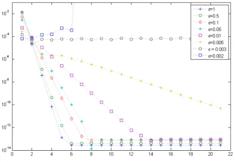
This is then extended to a full SDC predictor-corrector scheme and run for different values of to time t = 1. Figure 3.3 shows the error, compared to the exact solution g(t), and it is clear that as the stiffness of an ODE increases, more SDC iterations are

necessary for full convergence, if it will converge at all.

There are a two key points that this example illustrates. First, that order of conver-gence for SDC methods applied to stiff problems is a function of the number of iterations and the stiffness of the problem. Second, that this dependence on stiffness appears to be on a continuum, i.e. the stiffer the problem, the more SDC iterations needed for convergence, if it will converge at all.

Additionally, it should be noted that this issue was addressed by Huanget. al., where GMRES Krylov subspace methods were employed to successfully accelerate the conver-gence of SDC, giving near full order under certain conditions [51]. The order is still reduced, because the problem is stiff, however it is not an artifact of the treatement of the method [45]. Although this technique is not used here, a more robust picture of

(40)

Figure 3.3. Number of SDC correction sweeps vs. error, solving (3.34)

with different ’s

(41)

CHAPTER 4

Spatial Splitting in BPM

As previously discussed, the source of stiffness for both IBM and BPM is due to the presence of fiber forces. The force itself is local to the fiber and although the projection of the force is a global function, most of the magnitude of _Pfff is near the fiber. Thus the effects of _Pfff away from the fiber is not as large. Overall, the locally spatial behavior of the projection of the forces lends itself to the idea of splitting up the spatial field. This can be done with BPM, unlike IBM, since _Pfff can be analytically defined everywhere. This chapter will present a spatial splitting of _Pfff, with the intention that the local, stiff part will be evaluated with a different technique than that used for the non-stiff, non-local part.

4.1. Splitting _Pfff

In order to decompose how _Pfff effects the FSI equations, a quantitative metric for stiffness from this term is necessary. Here, spring forces and bending forces are used, as have been seen in application [21, 68]. The dependence of stiffness is linked to the spring constant, and in turn the spring constant scales directly with both the magnitude of

(42)

Figure 4.1. Scaling ofPfff and ∇Pfff with the spring constant k

The splitting discussed in this section will be of the spatial domain (Γ∪ Ω, with definitions on both Γ and Ω, and will consist of two domains, the near fieldandfar field. The near field is taken as the compact area near the boundary and designed to capture most of the stiffness. The far field is a smooth representation of _Pfff on Ω near Γ and away from it does not change rapidly, thus can be considered non-stuff. Thus, _Pfff is decomposed into

(4.1) _Pfff =nf+ff,

with

near field : nf =_Pfff −HR(r),

(4.2)

far field : ff =_Pfff −nf =HR(r),

(4.3)

whereHR(r) is an approximation function and R is the radius of the near field in terms

of δ. That is, for a near field defined as the area within 3δ of each fiber point, R = 3 and the corresponding approximation function is denoted, HR=3(r). Note that both the near and far field are defined with the choice of HR(r), thus this term will be examined

(43)

(a) p1(r) (b)p2(r)

Figure 4.2. The two radially symmetric terms ofPfff, for a fixedδ

4.1.1. Defining HR(r). There are two main constraints that guide the construction of

the near field. First, this quantity should capture the majority of the stiffness. Second, when it is used to construct the far field, ff = _Pfff −nf, the subtraction of the local nf

from the global_Pfff, should not leave any analytic discontinuities.

As discussed in section 2.3, BPM analytically defines_Pfff at any arbitrary pointxxx on the grid, using the following sum over theNΓLagrangian fiber points, with corresponding position XXX. This is given here again for reference, for a fiber XXX ∈ _R2 _or _X_X_X _∈

R3with forcefff ∈_R3

Pfff =

NΓ

X

γ=0

r_F0(r)−_F(r) 2πr2

fff_γ∆l−

r_F0(r)−2_F(r) 2πr2

ˆ x x

xγ(fffγ∆l·xxˆxγ),

(4.4)

where _F(r) = 2π Z r

0

sBδ(s)ds, r =|xxx−XXXγ|, xxˆx= (xxx−XXXγ)/r.

To define HR(r), first denote each radially symmetric term in (4.4), as p1(r) and p2(r), where

Pfff =

NΓ

X

γ=0

p1(r)fffγ∆l−p2(r)ˆxxxγ(fffγ∆l·xxˆxγ),

(44)

and

(4.5) p1(r) =

r_F0(r)−_F(r)

2πr2 , p2(r) =

r_F0(r)−2_F(r) 2πr2 .

These are shown in Fig. 4.2 and gives the following general form ofHR(r):

(4.6) HR(r) =

      

H1(r)fffγ∆l−H2(r)ˆxxxγ(fffγ∆l·xxxˆk) if r_δ >R,

Pfff if rδ ≤ R.

We choose H1(r) and H2(r) to be fourth degree polynomials of form

H1,2(r) = a1,2+b1,2

r δ

2

−(R)2

+c1,2

r δ

2

−(R)2 2

, (4.7)

with coefficients a1,2, b1,2, c1,2 for H1(r) and H2(r) respectively. These are constructed by the polynomial approximation technique of matching conditions. H1(r) will be con-structed matching the conditions of p1(r) and H2(r) matchingp2(r), which are given in detail in the following sections. This definition ofHR(r) gives the following definition of

the near field, which is indeed compact and local.

(4.8) nf =

      

Pfff −HR(r) if r_δ ≤ R,

0 if r_δ >R.

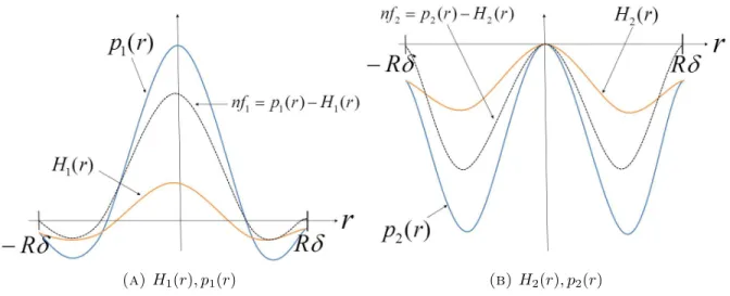
An example of H1(r), p1(r), H2(r), p1(r), p2(r) and their the resulting near field components are depicted in Figure 4.3.

4.1.2. Polynomial Approximation. To ensure that the near field is local, the match-ing value

(45)

(a) H1(r), p1(r) (b)H2(r), p2(r)

Figure 4.3. Components of the splitting function

is always used. To define the other matching conditions, the following parameters are needed for both H1(r) and H2(r)

R : the ratio of the radius of the near field andδ from each point on Γ, (4.10)

α1 : matching point where H1,2(α1) = p1,2(α1),respectively,

(4.11)

α2 : matching point where H10,2(α2) = p01,2(α2),respectively. (4.12)

To explore this parameter space, a Mathematica program was created, where R, α1 andα2 were variables. The range forα1andα2 was from 0 toRδ, stepping by increments of ₁₀1Rδ and for visual purposesδ= 1/100 was used to howα1 andα2 effected the scaling of the nf. Figures 4.4 - 4.5 show the result of this program with R= 1. In these figures, the orange line represents H1,2(r), the blue line is p1,2(r) and the dotted line is the resulting near field component nf₁_,₂. Additional figures for different cases of R can be found in the Appendix.

The dependence of the computational cost of the near field on R should be noted. The near field each is evaluated at each point defining Γ, XXX_γ, where the contribution from the pointsXXX_γ_˜, such that

||XXX_γ−XXX_˜_γ|| ≤ Rδ.

(46)

As R increases, a larger percentage of pointsXXX_γ_˜/NΓ contributes to this sum, thus the computational cost increases. This is revisited later when talking about specific tech-niques, but should be mentioned in context of an analysis of the near field.

(a) α1= 0 and α2= 0 (b)α1= 0.3δandα2= 0.6δ

Figure 4.4. H1(r) with R= 1 and labeled matching conditions

For eachR, four sets of matching conditions were chosen to compare. The choice was made for those values of α1 and α2 that captured the majority of the magnitude of the near field, while reducing the magnitude of the far field. These new values, as well as the coefficients a1,2, b1,2, c1,2 are given in Tables 4.1 and 4.2 and graphs of these conditions with R = 1 are given in Figures 4.6 and 4.7. Graphs of R = 2,3 with the conditions listed in Tables 4.1 and 4.2, respectively, can be found in the Appendix.

(47)

(a) α1=δandα2= 0.4δ (b)α1= 0.2δandα2= 5δ

Figure 4.5. H2(r) with R= 1 and labeled matching conditions

Initially the ellipse, immersed in a fluid at rest, is defined by the parametrization

(4.13) XXX(θ) = (r(θ) cos(θ−θ0), r(θ) sin(θ−θ0)),

where

r2(θ) = a2cos2(θ) +b2sin(θ) +

−4

3e

−3(θ−π)2

−e−5(θ−θ1)2 ₊_e−8(θ−θ2)2

.

The parameters used area= 0.2, b= 0.25, = 0.012, θ0 =π/3, θ1 = 4π/5, andθ2 = 2π/3. The grid is subdivided into Nx = Ny = 128 grid cells and the immersed boundary is

discretized by NΓ = 400 points, unless otherwise noted. Forces are defined by linear springs, with resting length zero and spring constant ks = 1010, attaching each point on

the immersed boundary.

SDC is used to preform the time integration withK = 3 SDC sweeps andM = 5 SDC nodes. The time step used is ∆tn= 0.00006, and the simulation evolves toT = 0.0006s.

The choice of time scale and ks are arbitrary, as using a smaller spring constant and

(48)

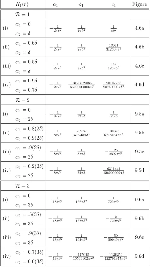
Table 4.1. Coefficients forH1(r)

H1(r) a1 b1 c1 Figure

R= 1

(i) α1 = 0 − 1

2πδ2

1 2πδ2

1

πδ2 4.6a

α2 =δ

(ii) α1 = 0.6δ − 1 2πδ2

1 2πδ2

13031

31250πδ2 4.6b

α2 =δ

(iii) α1 = 0.5δ − 1 2πδ2

1 2πδ2

149

128πδ2 4.6c

α2 =δ

(iv) α1 = 0.9δ − 1 2πδ2

13170879083 16600000000πδ2

20107253

20750000πδ2 4.6d

α2 = 0.7δ

R= 2

(i) α1 = 0 − 1

8πδ2

1 32πδ

1

64πδ 9.5a

α2 = 2δ

(ii) α1 = 0.8(2δ) − 1 8πδ2

26275 373248πδ2

100625

6718464πδ2 9.5b

α2 = 0.9(2δ)

(iii) α1 =.9(2δ) − 1 8πδ2

1

32πδ −

25

2592πδ2 9.5c

α2 = 2δ

(iv) α1 = 0.2(2δ) − 1 8πδ2

1 32πδ

6311441

128000000πδ 9.5d

α2 = 2δ

R= 3

(i) α1 = 0 − 1

18πδ2 ₁₆₂1_πδ2 ₇₂₉1_πδ2 9.6a

α2 = 3δ

(ii) α1 =.5(3δ) − 1 18πδ2

1

162πδ2 −

2

729πδ2 9.6b

α2 = 3δ

(iii) α1 =.9(3δ) − 1 18πδ2

1

162πδ2 −

50

59049πδ2 9.6c

α2 = 3δ

(iv) α1 = 0.7(3δ) − 1 18πδ2 −

175025 16503102πδ2 −

1126250

222791877πδ2 9.6d

(49)

(a) (b)

(c) (d)

Figure 4.6. H1(r) with R= 1 and matching conditions (i)-(iv), given in Table 4.1

longer time scale would produce the same problem. The initial configuration and the motion captured at T = 0.0006s later are shown in Figure 4.8.

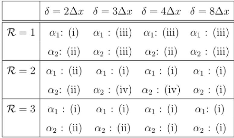
Two examples of the coefficient comparison tests are shown in Figures 4.9 and 4.10, more are seen in the Appendix. In these figures, the x axis is an index given by the condition case,C, such that if the cases forH1(r) are notatedc1 = 1,2,3,4,corresponding to cases i,ii,iii,iv, and similarly for H2(r), c2 = 1,2,3,4, then C = c2 + 4(c1 −1). The optimal coefficients, those that produce the largest ratio of |_Pfff|/|ff| and |∇_Pfff|/|∇ff|, are reported in Tables 4.3 - 4.6 for different cases, where ∆x is the grid size.

Tables 4.3 and 4.4 show that α1 does not vary with change in grid size, and does not vary acrossRat all, with the exception ofδ = 2∆xon a 256 grid. This is not an unusual case to see a difference because a blob radius of that size is more singular and not well

(50)

Table 4.2. Coefficients forH2(r)

H2(r) a2 b2 c2 Figure

R= 1

(i) α1 = 0 − 1

πδ2

1

πδ2

2

πδ2 4.7a

α2 =δ

(ii ) α1 = 0.3δ − 1

πδ2

1

πδ2

205951

200000πδ2 4.7b

α2 =δ

(iii) α1 = 0.3δ − 1

πδ2 −

3903971

5781250πδ2 −

6002981

7400000πδ2 4.7c

α2 = 0.6δ

(iv) α1 = 0.4δ − 1

πδ2

1

πδ2

1306

3125πδ2 4.7d

α2 =δ

R= 2

(i) α1 = 0 − 1 4πδ2

1 16πδ2

1

32πδ2 9.7a

α2 = 2δ

(ii) α1 = 0.9(2δ) − 1 4πδ2

1

16πδ2 −

25

1296πδ2 9.7b

α2 =δ

(iii) α1 = 0.5(2δ) − 1

4πδ2 −

1

2πδ2 −

1

4πδ2 9.7c

α2 = 0.5(2δ)

(iv) α1 = 0.1(2δ) − 1 4πδ2 −

38964269 142656250πδ2 −

997349

11412500πδ2 9.7d

α2 = 0.3(2δ)

R= 3

(i) α1 = 0 − 1 9πδ

1

81πδ2 ₇₂₉2_πδ2 9.8a

α2 = 3δ

(ii) α1 = 0.9(3δ) − 1 9πδ

1

81πδ2 −

100

59049πδ2 9.8b

α2 = 3δ

(iii) α1 = 0.5(3δ) − 1

9πδ −

8

81πδ2 −

16

729πδ2 9.8c

α2 = 0.5(3δ)

(iv) α1 = 0.7(3δ) − 1 9πδ −

200

194481πδ2 −

10000

1750329πδ2 9.8d

(51)

(a) (b)

(c) (d)

Figure 4.7. H2(r) with R= 1 and matching conditions (i)-(iv), given in Table 4.2

(a) t= 0 (b) t= 0.0006

Figure 4.8. Perturbed Ellipse.

(52)

resolved. For the case of α2, it has less uniform behavior. With large near field areas, such as R= 2 and δ= 4∆x on a 128×128 grid, orR= 3 and δ= 4∆x on a 256×256 grid, the optimal α2 almost always condition (i).

Figure 4.9. Coefficients with 128×128 grid, NΓ = 400 with δ= 4/128, and R= 1

Tables 4.5 and 4.6 show different grid sizes vs. gain from the optimal coefficients, measured by the ratio of |_Pfff /ff| and |∇_Pfff /∇ff|, with a δ that varied with grid size (Table 4.5), and with fixed δ= 4/128 (Table 4.6). Table 4.5 shows that the blob radius does not have a large effect on the on the gain from the splitting. Conversely, Table 4.12 shows that the gain achieved is proportional to the near field size, which would mean it

(53)

Table 4.3. Optimal coefficients for H1(r), H2(r) on a 128 x 128 grid

δ = 2∆x δ= 3∆x δ = 4∆x δ= 8∆x

R= 1 α1: (iii) α1 : (iii) α1: (iii) α1 : (iii) α2: (iii) α2 : (i) α2: (i) α2 : (i)

R= 2 α1 : (i) α1 : (i) α1 : (i) α1 : (i) α2: (iv) α2 : (iv) α2 : (i) α2 : (i)

R= 3 α1 : (i) α1 : (i) α1 : (i) α1: (i) α2 : (ii) α2 : (i) α2 : (i) α2 : (i)

Table 4.4. Optimal coefficients for H1(r), H2(r) on a 256 x 256 grid

δ = 2∆x δ= 3∆x δ = 4∆x δ= 8∆x

R= 1 α1: (i) α1 : (iii) α1: (iii) α1 : (iii) α2: (ii) α2 : (iii) α2: (ii) α2 : (iii)

R= 2 α1 : (ii) α1 : (i) α1 : (i) α1 : (i) α2: (ii) α2 : (iv) α2 : (iv) α2 : (i)

R= 3 α1 : (i) α1 : (i) α1 : (i) α1: (i) α2 : (ii) α2 : (ii) α2 : (i) α2 : (i)

does depend onR. This is to expected since a larger near field captures more effect from