umi-unc-2892.pdf

A M

etropolis

-H

astings

R

obbins

-M

onro

A

lgorithm for

M

aximum

L

ikelihood

N

onlinear

L

atent

S

tructure

A

nalysis with a

C

omprehensive

M

easurement

M

odel

Li Cai

A dissertation submitted to the faculty of the University of North Carolina at Chapel Hill in partial fulfillment of the requirements for the degree of Doctor of Philosophy in the Department of Psychology (Quantitative).

Chapel Hill 2008

Approved by

Robert C. MacCallum, Ph.D.

David M. Thissen, Ph.D.

Daniel J. Bauer, Ph.D.

Stephen H. C. du Toit, Ph.D.

c 2008

Li Cai

ABSTRACT

Li Cai: A Metropolis-Hastings Robbins-Monro Algorithm for Maximum Likelihood Nonlinear Latent Structure Analysis with a Comprehensive Measurement Model

(Under the direction of Robert C. MacCallum and David M. Thissen)

ACKNOWLEDGEMENTS

First and foremost, I would like to thank my advisors, Drs. Robert MacCallum and David Thissen, for their unwavering support and guidance over the years, and I thank members of my committee for the many stimulating discussions and sugges-tions that led to a much improved research project.

I thank my friends and colleagues at the Thurstone Psychometric Lab. I also thank Dr. Michael Edwards for kindly sharing his MultiNorm program and data sets. I am indebted to the many mathematicians and statisticians that worked on the theories of stochastic processes and optimization, and to computer scientists who helped create TEX, LA_{TEX, and C++. I would not have come this far intellectually}

without your insights.

Generous financial support from the Educational Testing Service (in the form of a Harold Gulliksen Psychometric Research Fellowship) and the National Science Foundation (Grant # SES-0717941) is gratefully acknowledged.

TABLE OF CONTENTS

List of Tables . . . ix

List of Figures . . . x

CHAPTER

1.1 Background . . . 2

1.1.1 Limited-information Categorical Factor Analysis . . . 4

1.1.2 Full-information Item Factor Analysis . . . 6

1.1.3 Random-Effects, Mixtures, and Latent Variables . . . 8

1.2 Numerical Integration in FIML . . . 10

1.2.1 Laplace Approximation . . . 11

1.2.2 Adaptive Quadrature . . . 11

1.2.3 Monte Carlo EM . . . 12

1.2.4 Simulated Maximum Likelihood and Variants . . . 13

1.2.5 Fully Bayesian MCMC . . . 14

1.3 Stochastic Approximation Algorithms . . . 15

2 A Latent Structure Model . . . 17

2.1 Latent Structural Models . . . 17

2.1.1 Linear Structural Model . . . 18

2.1.2 Nonlinear Structural Model . . . 18

2.2 Measurement Models . . . 19

2.2.2 Graded Response . . . 20

2.2.3 Nominal Response . . . 21

2.2.4 Continuous Response . . . 23

2.3 Observed and Complete Data Likelihoods . . . 23

2.3.1 Observed Data Likelihood . . . 23

2.3.2 Complete Data Likelihood . . . 24

3 A Metropolis-Hastings Robbins-Monro Algorithm . . . 26

3.1 The EM Algorithm and Fisher’s Identity . . . 26

3.2 MH-RM as a Generalized RM Algorithm . . . 27

3.3 Relation of MH-RM to Existing Algorithms . . . 30

3.4 The Convergence of MH-RM . . . 31

3.5 Approximating the Information Matrix . . . 32

4 Implementation of MH-RM . . . 34

4.1 A Metropolis-Hastings Sampler . . . 34

4.2 Complete Data Models and Derivatives . . . 37

4.2.1 Linear Latent Structure . . . 38

4.2.2 Nonlinear Latent Structure . . . 39

4.2.3 Dichotomous Response with Guessing Effect . . . 40

4.2.4 Graded Response . . . 42

4.2.5 Nominal Response . . . 43

4.2.6 Continuous Response . . . 45

4.3 Acceleration and Convergence . . . 45

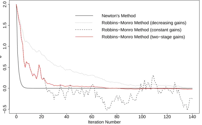
4.3.1 Adaptive Gain Constants . . . 45

4.3.2 Multi-stage Gain Constants . . . 46

4.3.3 Convergence Check . . . 47

5 Applications of MH-RM . . . 49

5.1 One-Parameter Logistic IRT Model for LSAT6 Data . . . 49

5.3 Four-Dimensional Confirmatory Item Factor Analysis . . . 51

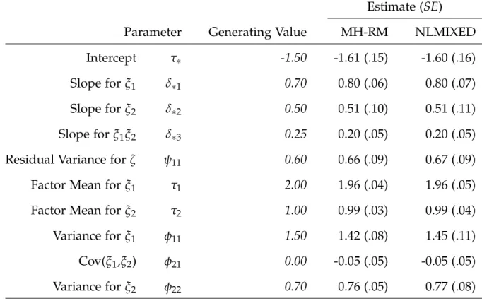
5.4 Latent Variable Interaction Analysis . . . 52

5.5 Latent Mediated Regression with Dichotomous Indicators . . . 54

5.6 Full-information Estimation of Tetrachoric Correlations . . . 58

5.6.1 An Approach Using Underlying Response Variates . . . 59

5.6.2 An Approach Using Logistic Approximation . . . 62

5.6.3 An Example . . . 63

6 Preliminary Sampling Experiments with MH-RM . . . 72

6.1 A Unidimensional Model . . . 72

6.2 A Constrained Multidimensional Nominal Model . . . 78

6.3 A Bifactor Type Model for Graded Responses . . . 80

7 Discussions and Future Directions . . . 94

7.1 Discussions . . . 94

7.2 Future Directions . . . 95

LIST OF TABLES

5.1 LSAT6 One-Parameter Logistic Model Estimates . . . 65

5.2 LSAT6 Three-Parameter Logistic Model Estimates . . . 65

5.3 Four-Dimensional Item Factor Analysis: Factor Correlation Estimates . . . 65

5.4 Four-Dimensional Item Factor Analysis: Item Parameter Estimates . . . 66

5.5 Latent Variable Interaction: Structural Model Estimates . . . 67

5.6 Latent Variable Interaction: Measurement Model Estimates . . . 68

5.7 Latent Mediated Regression: Measurement Intercept Generating Values . . 68

5.8 Latent Mediated Regression: Measurement Slope Generating Values . . . . 69

5.9 Latent Mediated Regression: Structural Model Estimates . . . 69

5.10 Generating Tetrachoric Correlations and Thresholds . . . 70

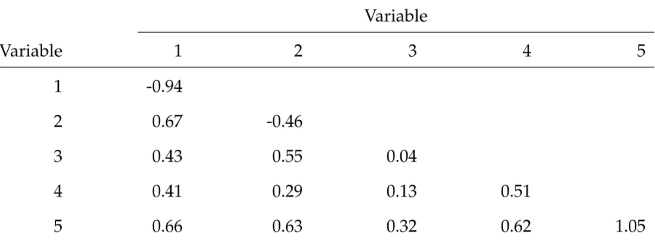
5.11 Means and Pearson Correlations of the Underlying Response Variables . . 70

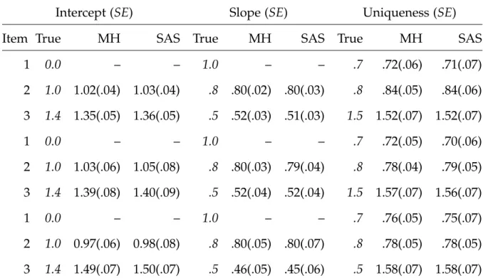
5.12 Comparison of Three Estimation Methods for Tetrachoric Correlations . . . 71

6.1 Timing the MH-RM for Unidimensional IRT Simulation . . . 84

6.2 Unidimensional IRT Model (N =200) . . . 85

6.3 Unidimensional IRT Model (N =1000) . . . 86

6.4 Unidimensional IRT Model (N =3000) . . . 87

6.5 Multidimensional Nominal Model: Slopes . . . 88

6.6 Multidimensional Nominal Model: Factor Correlations . . . 89

6.7 Multidimensional Nominal Model: αand γ Estimate and Bias . . . 90

6.8 Multidimensional Nominal Model: αand γ Standard Errors . . . 91

6.9 Generating Parameter Values for the Bifactor Type Model: Items 1–23 . . . 92

LIST OF FIGURES

4.1 The Effect of Gain Constants on the Robbins-Monro Iterations . . . 48

5.1 Path Diagram for Confirmatory Item Factor Analysis . . . 51

5.2 Path Diagram for Latent Variable Interaction . . . 54

5.3 Path Diagram for Latent Mediated Regression . . . 56

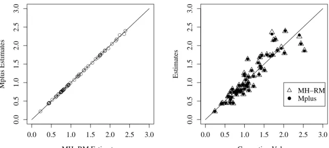
5.4 Latent Mediated Regression: Intercept Estimates . . . 57

5.5 Latent Mediated Regression: Slope Estimates . . . 57

6.1 Unidimensional IRT Model (N =200): Intercepts . . . 75

6.2 Unidimensional IRT Model (N =200): Slopes . . . 75

6.3 Unidimensional IRT Model (N =1000): Intercepts . . . 76

6.4 Unidimensional IRT Model (N =1000): Slopes . . . 76

6.5 Unidimensional IRT Model (N =3000): Intercepts . . . 77

6.6 Unidimensional IRT Model (N =3000): Slopes . . . 77

6.7 Path Diagram for A Constrained Multidimensional Nominal Model . . . . 78

6.8 Path Diagram for a Bifactor Type Model for Graded Responses . . . 80

6.9 Bifactor Type Model: Intercepts . . . 82

6.10 Bifactor Type Model: Slopes for the Primary Dimension . . . 83

CHAPTER 1

Introduction

In the present research, latent structure model refers to a class of parametric sta-tistical models that specify linear or nonlinear relations among a set of continuous latent variables. The term is admittedly influenced by Lazarsfeld’s (1950) chapter on latent structure analysis, although only continuous latent traits will be consid-ered in the sequel. The observed variables become indicators of the latent variables via a comprehensive measurement model such that an arbitrary mixture of metric and non-metric variables is permitted at the manifest level, including e.g., dichotomous, ordered polytomous, and nominal responses.

For a variety of technical reasons, it is a preferable practice that all parameters in the latent structure model be jointly estimated using full-information maximum likelihood (FIML). However, the likelihood function of the latent structure model involves intractable high dimensional integrals that present serious numerical chal-lenges. For standard Gaussian quadrature based methods, the amount of computa-tion increases exponentially as a funccomputa-tion of the number of latent variables. This is known in the literature as the “curse of dimensionality.” Existing Monte Carlo based methods also become cumbersome when both the number of latent variables and the number of observed variables are large.

2006) and apply it to solve the parameter estimation problem in maximum likeli-hood latent structure modelling. The MH-RM algorithm combines the Metropolis-Hastings (MH; Metropolis-Hastings, 1970; Metropolis, Rosenbluth, Rosenbluth, Teller, & Teller, 1953) algorithm and the Robbins-Monro (RM; Robbins & Monro, 1951) stochastic ap-proximation (SA; see e.g., Kushner & Yin, 1997) algorithm. The MH-RM algorithm was initially proposed by Cai (2006) for exploratory item factor analysis. A general convergence proof has been worked out and MH-RM performed satisfactorily in pre-liminary comparisons against leading item factor analysis software packages. MH-RM can handle large-scale analysis with many items, many factors, and thousands of respondents. It is flexible enough to seamlessly incorporate the mixing of different item response models, missing data, and multiple groups. It is well-suited to gen-eral computer programming for confirmatory analysis with arbitrary user-defined constraints. It is efficient in the use of Monte Carlo and unlike the EM algorithm it also produces an estimate of the parameter information matrix as an automatic by-product.

MH-RM has the potential of becoming a general and self-adaptive algorithm for arbitrarily high dimensional latent trait analysis. While the use of MH-RM is novel in its own right, a significant by-product of the present research is the integration of research on the parametrization and estimation of complex nonlinear latent variable models. To that end, a review of relevant background information is in order.

1.1 Background

1966; Bollen, 1989; J ¨oreskog, 1970), and item response theory (Lord & Novick, 1968; Thissen & Wainer, 2001). To the applied statistician, latent structure models are de-scribed in a distinctly modern statistical language, using the general framework of hierarchical models (see e.g., Bartholomew & Knott, 1999). These models offer fertile new ground for interesting applications of modern statistical and computational the-ory (see e.g. Dunson, 2000 for a statistician’s view on latent variable models). To the statistical software programmers, the advent of a general modelling framework per-mits the development of general software packages that combine features of existing software such as Lisrel (J ¨oreskog & S ¨orbom, 2001), Testfact (Bock et al., 2003), and Multilog (Thissen, 2003). To administrators of testing programs and ultimately test users, latent structure models provide essential tools for item analysis, test assembly, and score reporting. For instance, as noted by von Davier and Sinharray (2004), the reporting methods used in NAEP rely on a special multidimensional item response model with covariate effects.

Latent structure models have been invented (and reinvented) under many differ-ent names. However, three main currdiffer-ents of research can be iddiffer-entified:

1. the extension of factor analysis and structural equation modelling to categorical indicators,

2. the growth of multidimensional item response theory (IRT), especially full-information item factor analysis (FIFA), and

3. the infusion of statistical concepts such as hierarchical models, mixture models, and mixed-effects models into psychometrics.

1.1.1 Limited-information Categorical Factor Analysis

Limited-information methods have a long tradition in psychometrics. This line of work began with the now classical treatment of factor analysis of categorical data by Christoffersson (1975) and Muth´en (1978). It was soon realized that Muth´en’s (1978) approach could handle far richer structural models than the common factor model. Indeed, Muth´en (1984) showed later that J ¨oreskog’s (1970) linear structural model could be generalized to the case of mixed continuous and ordinal outcomes.

Building upon the equivalence of the “underlying response” formulation and the IRT formulation of categorical factor analysis (Takane & de Leeuw, 1987), several multi-stage estimators based on univariate and bivariate (hence limited) informa-tion have been proposed (e.g., Lee, Poon, & Bentler, 1992, 1995a, 1995b; Muth´en & Muth´en, 2007), and they compared favorably in empirical research against optimal but more computationally demanding estimators such as full information maximum likelihood (see e.g., Bolt, 2005; Knol & Berger, 1991). These estimators share the com-mon feature that estimates of the category thresholds and polychoric correlations are obtained in the first one or two stages, as well as the asymptotic covariance matrix of these estimates. In the final stage, the remaining structural parameters are estimated using generalized least squares (GLS).

As far as statistical theory is concerned, these GLS-based estimators are grounded on sound principles. Furthermore, they have important ties to Browne’s (1984) asymptotically distribution free method for moment structures, also known as the method of estimating equations in the statistical literature (Godambe, 1960) and the generalized method of moments in the econometric literature (Hansen, 1982). The concept of limited-information has also motivated recent development of goodness-of-fit indices for categorical data models (e.g., Bartholomew & Leung, 2002; Cai, Maydeu-Olivares, Coffman, & Thissen, 2006; Maydeu-Olivares & Joe, 2005).

polychoric/polyserial correlations, so the resulting polychoric correlation matrix may not be positive definite. It is interesting to note that the dependence on pair-wise es-timation is also a consequence of the “curse of dimensionality.” Obtaining a full polychoric/polyserial correlation matrix by maximum likelihood requires as many dimensions of numerical integration as the number of observed variables, which is typically large. In addition, if the sample size is not too large, the asymptotic covari-ance matrix of the polychoric correlations cannot be determined accurately, which may adversely affect the GLS estimation of structural parameters. Although remedies such as the diagonally weighted least squares estimator appear to work in practice (see e.g., Flora & Curran, 2004 for recent simulation results), current implementa-tions of these estimators often require ad hoc corrections for zero cell-counts in the marginal contingency tables. Furthermore, computation can become intense if the number of observed variables is large. To a psychometrician, the main drawback of GLS-based methods is the complete lack of support of other (more interesting) types of measurement models, such as the nominal model (Bock, 1972), not to mention the awkwardness when missing responses are present. Finally, due to the multi-stage nature of the estimation procedure, a fully Bayesian analysis is cumbersome. A no-table exception to the above criticism is the Monte Carlo EM method for estimating polychoric correlations due to Song and Lee (2003), but this method is based on FIML so that one might as well estimate the structural parameters directly, with even lower dimensional integrals to solve.

would be well over 1000 parameters to be jointly estimated. As will be shown, joint optimization of all parameters is unnecessary, but the current UBN formulation does not shed light on how the problem may be justifiably reduced to lower dimensions.

It should be noted that McDonald’s (1967) treatise on nonlinear factor analysis and the associated NOHARM software (Fraser & McDonald, 1988) for parameter es-timation can also be classified as using limited-information. However, the NOHARM method is based on ordinary least squares, and it is not even efficient among the class of limited-information estimators. This method has also seen limited practical use.

General latent structure models have taken preliminary shape within the limited-information approach. The GLS-based estimation method has enjoyed a high degree of popularity among practitioners over the past decades partly because of the ex-istence of successful software programs such as Lisrel or Mplus. Many interesting applications ensued, but it can be concluded from examining the trend of recent re-search that traditional GLS-based estimation methods have failed to keep up with the ever-increasing complexity of measurement and structural models.

1.1.2 Full-information Item Factor Analysis

Occurring around the same period as Muth´en (1978) proposed the GLS estimator, Bock and colleagues popularized the maximum marginal likelihood (MML) estimator in the field of IRT (Bock & Aitkin, 1981; Bock & Lieberman, 1970; Thissen, 1982). This estimator uses full-information and circumvents many problems associated with the limited-information approach. It eventually led to active research on FIFA (Bock, Gibbons, & Muraki, 1988; Gibbons et al., 2007; Meng & Schilling, 1996; Mislevy, 1986; Muraki & Carlson, 1995; Schilling & Bock, 2005). Wirth and Edwards (2007) provide a recent overview of FIFA.

It provides a wealth of information about scale dimensionality and item appropriate-ness, and it has also been used widely as a tool for modelling local dependence, e.g., testlets (Wainer & Kiely, 1987).

While standard IRT models are unidimensional in the sense that only one fac-tor is in the model, recent applications of IRT in domains such as personality and health outcomes (see e.g., Bjorner, Chang, Thissen, & Reeve, 2007; Reeve et al., 2007; Reise, Ainsworth, & Haviland, 2003; Thissen, Reeve, Bjorner, & Chang, 2007) have prompted the increasing use of FIFA. However, the MML method leads to analyti-cally intractable high dimensional integrals in the likelihood function, which is al-ready nonlinear. The difficult nonlinear optimization problem is further complicated by the fact that there are typically many items and many respondents in applica-tions of FIFA. Thus the use of standard Newton-type algorithms for maximizing the FIFA log-likelihood, e.g., Bock and Lieberman (1970), does not generalize well to real psychological and educational testing situations.

A break-through was made when Bock and Aitkin (1981) proposed a quadrature based EM algorithm. The main idea of Bock and Aitkin (1981) is remarkably simple: in step one, “make up” artificial data by conditioning on provisional estimates and observed data; step two, estimate parameters and go back to step one and repeat until parameters do not change further. This paper not only made important contributions to the computational methods of the day and established the de facto standard of parameter estimation method in the IRT field for the next two and half decades, but it was also profoundly influential in helping shape psychometricians’ view on latent variable models. Evidence of its lasting impact is provided by over 400 citations since its publication, in fields ranging from education and psychology to biostatistics and medicine.

instance, their empirical characterization of the latent ability distribution is at the crossroads of latent trait models and latent class models. The model for structured item parameters is effectively a Multiple-Indicator Multiple-Cause (MIMIC; see e.g., Bollen, 1989) model, widely known in the structural equation modelling community. Because of the IRT orientation of FIFA, the kinds of structural models in widespread use are usually not as rich as those seen in the categorical factor analysis and structural equation modelling domain. The difference can be attributed to the difficulty of numerically evaluating high dimensional integrals in the EM algorithm for FIFA. The so-called “curse of dimensionality” is partially alleviated with recent development in statistical computing, especially Markov chain Monte Carlo (MCMC; see e.g., Tierney, 1994).

A clear trend that began with Albert’s (1992) Bayesian analysis of the two-parameter normal ogive IRT model has been the wider acceptance of MCMC-based estimation algorithms in FIFA (B´eguin & Glas, 2001; Edwards, 2005; Meng & Schilling, 1996; Patz & Junker, 1999a, 1999b; Segall, 1998; Shi & Lee, 1998). These developments blurred the boundaries between traditional domains of psychometrics such as IRT and structural equation modelling. Equipped with powerful modern computational methods and converging theories on latent variables models, general latent structure models have finally come to fruition.

1.1.3 Random-Effects, Mixtures, and Latent Variables

instance, in a series of papers, Fox and colleagues have developed a multilevel IRT model (Fox, 2003, 2005; Fox & Glas, 2001) that is a synthesis of IRT and random effects regression models.

The literature has reached a consensus that latent variables are synonymous with random coefficients, factors, random effects, missing data, counterfactuals, unob-served heterogeneities, hidden volatilities, disturbances, errors, etc. The fact that they are known by different names is mostly a disciplinary terminology issue rather than real difference in their nature. In addition, it is not useful to classify models based on the type of observed variables. For a vector of observed variables, say,

y = (y1, . . . ,yn)0 that possesses density f(y), all latent variable models can be

ex-pressed as (cf. Bartholomew & Knott, 1999): f(y) =

Z

f(y|x)h(x)dx, (1.1) where x = (x1, . . . ,xp)0 is a p-dimensional vector of latent variables, f(y|x) the

con-ditional density of observed variables given latent variables, and h(x) the density of the latent variables. The y’s need not be all continuous, and neither must all the x’s be so. The p-fold integral over x can also be a mixture of integration and sum-mation, as dictated by the type of random variables. Note that the term density is used generically to refer to either the probability density function of an absolutely continuous random variable or the probability mass function of a discrete random variable. One need not distinguish between the two because conceptually they are both Radon-Nikodym derivatives of probability measures.

Equation (1.1) is of fundamental importance so comments are in order. First, the latent variable model is not uniquely determined. Any arbitrary transformation of x

of the exponential family while restricting x to have an absolutely continuous mul-tivariate distribution. This specification affords enough flexibility (as far as the role of latent traits in mental test theory is concerned) and translates into easily inter-pretable parameters. Second, f(y)is of the form of a mixture distribution, where the conditional density f(y|x) is mixed over h(x). This implies that unless f(y|x) and h(x) form conjugate pairs, the resulting integral does not have closed-form solution and must be approximated numerically. Third, Equation (1.1) has a hierarchical in-terpretation, wherein h(x) may be conceived of as a “prior” density that completes the specification of a Bayesian two-level model. In a similar vein, the x’s can also be thought of as nuisance parameters or random effects that must be integrated out to arrive at a genuine likelihood. This is the statistical basis for MML estimation. Finally, as the third point suggests, all inferences about x should be based on the posterior distribution f(x|y). For instance, the best mean square predictor ofxis the posterior mean, a fact well-utilized in normal theory linear mixed models (Harville, 1977) and IRT scoring (Thissen & Wainer, 2001).

The historical circle that began with Thurstone (1947), Lazarsfeld (1950), and Lord and Novick (1968) is finally complete. Now that Equation (1.1) provides a general setup for latent variable models and the role of maximum likelihood estimation, the immediate central issue becomes one of computation, especially methods for evaluating multidimensional integrals.

1.2 Numerical Integration in FIML

into five classes, with a gradation from deterministic to stochastic.

1.2.1 Laplace Approximation

This class of methods is characterized by the use of Laplace approximation (Tierney & Kadane, 1986). Psychometric applications of this method can be found in Kass and Steffey (1989) and Thomas (1993). The Laplace method is fast (see e.g., Raudenbush, Yang, & Yosef, 2000, in a slightly different application), but a notable feature of this method is that the error of approximation decreases only as the number of observed variables increases. When few items are administered to each examinee, such as in an adaptive test design, or when there are relatively few items loading on a factor, such as in the presence of testlets (Wainer & Kiely, 1987), the degree of imprecision in approximation can be substantial and may lead to biased param-eter estimates. Raudenbush et al. (2000) argue for the use of higher-order Laplace approximation, but the complexity of software implementation grows dramatically as the order of approximation increases. In addition, the truncation point in the asymptotic series expansion (6th-degree in their paper) of the integrand function is essentially arbitrary. Furthermore, from the perspective of random effects models, it is well known that if the error of approximation depends on cluster size (which is the same as the number of observed variables in this context), the standard Laplace method cannot be applied to models with crossed random effects (e.g., Kuk, 1999).

1.2.2 Adaptive Quadrature

quadrature rules do not accurately capture its mass. With care in implementation, pointwise convergence of the estimates to a local maximum of the likelihood func-tion can be obtained when an efficient quadrature rule is used in conjuncfunc-tion with either a Newton-type algorithm or the EM algorithm. Because of over two decades of success of Gaussian quadrature in IRT, it is often considered a gold standard against which other methods are compared. However, quadrature-based algorithms, e.g., those implemented in Testfact (Bock et al., 2003) or Gllamm (Rabe-Hesketh, Skron-dal, & Pickles, 2004), are still quite limited in the number of factors that they can handle simply because the number of quadrature points must grow exponentially as the dimensionality of the latent traits increases. In addition, because the EM al-gorithm does not provide information on sampling variability upon convergence, Testfact does not provide standard errors.

1.2.3 Monte Carlo EM

This class of methods is intimately related to Wei and Tanner’s (1990) MCEM algorithm, wherein Monte Carlo integration replaces numerical quadrature in the E-step (e.g., Meng & Schilling, 1996; Song & Lee, 2005). The latent variables are treated as missing data, and their plausible values are multiply imputed from the posterior predictive distribution f(x|y)of the missing data given the observed data and provi-sional estimates. As it will become clear in section 3, the connection between MCEM and likelihood-based approaches to missing data (e.g., Little & Rubin, 1987; Schafer, 1997) provides a strong motivation for the MH-RM algorithm.

As far as estimation is concerned, MCEM is inefficient in the use of simulated data because a new set of random draws are generated at each E-step, discarding all previous draws. Experience with the design of IRT estimation software that imple-ments the EM algorithm such as Multilog (Thissen, 2003) suggests that the E-step is usually much more time consuming than the M-step due to expensive exponential function calls and nested loop operations over both N and n. It is therefore not sur-prising that the E-step simulations in MCEM should take much more time than any other step. Discarding random draws appears to waste much needed computational resources and is clearly undesirable.

1.2.4 Simulated Maximum Likelihood and Variants

While quadrature-based EM and MCEM work on the log of the marginal like-lihood function, Geyer and Thompson’s (1992) simulated maximum likelike-lihood ap-proach seeks a direct Monte Carlo approximation to the marginal likelihood using importance sampling. The simulated likelihood is then optimized using standard numerical techniques such as Newton-Raphson. The appeal of simulated maximum likelihood is that in theory simulation is done only once, at the beginning of the es-timation algorithm. However, the resulting estimates become sensitive to the initial approximation to the likelihood, especially the choice of the importance sampling distribution. This leads to alternative, doubly-iterative procedures in which param-eters of the importance sampling distribution are updated after each optimization step. McCulloch and Searle (2001) advise caution on the implementation of simu-lated maximum likelihood, and Jank (2004) show that simusimu-lated maximum likeli-hood tends to be less efficient than MCEM. The details are too intricate and beyond the scope of the present research but briefly, one must pay close attention to the bal-ance of simulation size and the updating of the importbal-ance sampling distribution to ensure convergence (Capp´e, Douc, Moulines, & Robert, 2002).

Sample Average Approximation (SAA) method. SAA is not doubly-iterative. Return-ing to the log of the likelihood function, SAA exploits the structures of some latent variable models and uses Monte Carlo or quasi-Monte Carlo sampling from h(x) to directly approximate the log-likelihood. For instance, Qian and Shapiro (2006) con-sidered exploratory FIFA of dichotomous items. SAA is relatively new and holds promise for a class of relatively simple latent variable models wherein the mixing density h(x) does not contain parameters. However, for more general models the performance of SAA is unknown. It is also subject to the same criticism as the UBN approach (J ¨oreskog & Moustaki, 2001) in the sense that the size of the optimization problem in SAA can become unnecessarily large (if n is large) because SAA fails to exploit the conditional independence structure often encountered in models aris-ing out of test theory. Furthermore, SAA (in its original form in Qian & Shapiro, 2006) obscures the important connection between missing data imputation and latent variable modelling as the integration is taken with respect toh(x)instead of f(x|y).

1.2.5 Fully Bayesian MCMC

implementa-tions have not been entirely settled (see e.g., Edwards, 2005). In addition, great care and experience are needed to handle the numerical results because the chains only converge weakly and the use of convergence diagnostics can be cumbersome with models having both largen and p.

1.3 Stochastic Approximation Algorithms

From the preceding discussion, it seems clear that a flexible and efficient algo-rithm that converges pointwise to the the maximum likelihood estimate is much de-sired for high dimensional latent structural analysis. Indeed, in the research reported here, the MH-RM algorithm is suggested to address most of the afore-mentioned dif-ficulties. The MH-RM algorithm was initially proposed by Cai (2006) for exploratory FIFA and it compared favorably against leading IRT parameter estimation software packages in preliminary investigations.

The MH-RM algorithm is well-suited to general computer programming for high dimensional analysis with large n, p, and N. It is efficient in the use of Monte Carlo because the simulation size is fixed and usually small throughout the iterations. In addition, it also produces an estimate of the parameter information matrix as a by-product that can be used subsequently for standard error estimation and goodness-of-fit testing (e.g., Cai et al., 2006).

CHAPTER 2

A Latent Structure Model

Consistent with the review of historical background in Chapter 1, the latent struc-ture model considered here can be regarded either as a generalization of categorical structural equation models or as an extension of multidimensional IRT models. As a structural equation model, it not only incorporates a full Lisrel-type latent regres-sion model, but also permits nonlinear latent regresregres-sions such that polynomial and interaction effects between latent variables can be assessed. However, it differs from Arminger and Muth´en’s (1998) and Lee and Zhu’s (2000) nonlinear models in that the measurement part is developed directly from multidimensional IRT. For instance, the current framework includes a dichotomous IRT model with respondent guessing ef-fect, as well as a multidimensional nominal model (Thissen, Cai, & Bock, 2006). Both models are rarely discussed in the categorical factor analysis and structural equation modelling literature.

2.1 Latent Structural Models

Recall that there are N independent respondents,n observed variables or items, and p latent variables. Let the vector of latent variables for respondent i be denoted as xi. For convenience, the p-dimensional vector xi is further partitioned into two

sub-vectors: ξ_i (p1×1) and η_i (p2×1), such that xi = (ξ0_i,η0_i)0 and p = p1+p2. As

2.1.1 Linear Structural Model

A linear structure is assumed forξ_i:

ξ_i =τ+∆ξ_i+εi, (2.1)

whereτ is a p1×1 vector of latent variable means,∆is a p1×p1matrix of regression

coefficients, and εi is a p1×1 vector of multivariate normally distributed error terms

with zero means and covariance matrix Φ. Equation (2.1) represents a standard sys-tem of linear equations amongξ_i. It is further assumed that (Ip₁−∆) is nonsingular so thatξ_i can be expressed as

ξ_i = (Ip1 −∆)

−1₍

τ+εi). (2.2)

Upon defining A = (Ip1 −∆)

−1_{, Equation (2.2) implies that the distribution of ξ}

i is

p1-variate normal with meanAτ and covariance matrix AΦA0:

ξ_i ∼ Np1(Aτ,AΦA0) (2.3)

2.1.2 Nonlinear Structural Model

The latent variables inη_i are endogenous and are assumed to follow a nonlinear regression equation:

η_i =τ∗+∆∗g(ξ_i) +ζ_i, (2.4) where g(·) is a continuous vector-valued nonlinear function that maps the p1

-dimensional vector ξ_i into a q-dimensional vector g(ξ_i), and τ∗ is a p2×1 vector

of intercepts,∆∗ a p2×q matrix of regression coefficients. Finallyζ_i is a p2×1 vector

of normally distributed error terms that is uncorrelated with εi and has zero means

and covariance matrixΨ:

ζ_i ∼ Np2(0,Ψ). (2.5)

For computational reasons, it is convenient to define

Π =



 

τ0∗

∆0 ∗





, ξ∗i = 

 

1 g(ξ_i)





 (2.6)

and rewrite Equation (2.4) as:

η_i =Π0ξ_∗i+ζ_i. (2.7) Equation (2.7) implies that conditional on ξ∗i, the distribution of ηi is p2-variate

nor-mal with meanΠ0ξ∗i and covariance matrixΨ:

η_i|ξ_∗i ∼ Np2(Π

0

ξ_∗i,Ψ). (2.8)

2.2 Measurement Models

The measurement models are developed as multidimensional IRT models. The basic principle of conditional independence (Lord & Novick, 1968) is assumed. De-note the ith respondent’s vector of responses to the set of n observed variables as

y_i = (yi1, . . . ,yij, . . . ,yin)0. The conditional independence assumption states that

con-ditional on the respondent’s latent trait level x_i, the yij’s are mutually independent.

Therefore, it is sufficient in the sequel to consider measurement models for a single response yij to a generic item j. Before embarking on model development, it is also

useful to define an indicator function for categorical response models

χk(y) =

(

1, ify =k, 0, otherwise,

(2.9)

for nonnegative integerk ∈ {0, 1, 2, . . .}.

2.2.1 Dichotomous Response with Guessing Effect

This model is a generalization of the so-called 3-parameter logistic model (3PL) in unidimensional IRT. Givenxi, the conditional probability of observing yij =1 is

P(yij =1|xi,θj) =c(κj) + 1

−c(κj)

1+exp[−(γj+β0_jxi)]

where θj = (γj,β0_j,κj)0 is a(p+2)×1 vector of parameters with γj being the

inter-cept, β_j the p×1 vector of slopes, and c(κj) the so-called guessing parameter, where κj is the logit of guessing:

c(κj) =

1

1+exp(−κj). (2.11)

The logit reparametrization transforms a bounded parameter space to an unbounded one, and is customarily done in standard IRT software packages, e.g., Multilog (Thissen, 2003). Given Equation (2.10), the conditional probability of observing yij =0 is equal to

P(yij =0|xi,θj) =1−P(yij =1|xi;θj). (2.12)

The conditional density foryij is that of a Bernoulli variable:

f(yij|xi,θj) = P(yij =1|xi,θj)yijP(yij =0|xi,θj)1−yij. (2.13)

2.2.2 Graded Response

This model is the multidimensional counterpart of Samejima’s (1969) graded re-sponse model. Let yij ∈ {0, 1, 2, . . . ,Kj−1} be the response from respondent i to

item j in Kj ordered categories. The development starts from defining the following

logistic conditional cumulative response probabilities for each category:

P(yij ≥0|xi,θj) = 1,

P(yij ≥1|xi,θj) =

1

1+exp[−(γ1,j+β0_jxi)]

,

P(yij ≥2|xi,θj) =

1

1+exp[−(γ2,j+β0jxi)]

, ..

.

P(yij ≥Kj−1|xi,θj) = 1

1+exp[−(γKj−1,j+β

0

jxi)]

, (2.14)

where θj = (γ0_j,β0_j)0 is a (p +Kj − 1) ×1 vector of parameters, and γ_j =

implies that the category response probability is the difference between two adjacent cumulative probabilities:

P(yij =k|xi,θj) = P(yij ≥k|xi,θj)−P(yij ≥k+1|xi,θj), (2.15)

where P(yij ≥ Kj|xi,θj) is identically equal to zero to ensure Equation (2.15) is

well-defined for k = 0, 1, 2, . . . ,Kj−1. With the indicator function defined in Equation

(2.9), the conditional density foryij is a multinomial with trial size 1 inKj categories:

f(yij|xi,θj) =

Kj−1

∏

k=0

P(yij =k|xi,θj)χk(yij). (2.16)

2.2.3 Nominal Response

This model is a recent reparametrization of Bock’s (1972) original nominal model (Thissen et al., 2006). Let yij ∈ {0, 1, 2, . . . ,Kj−1} be the response from respondent

i to item j in Kj nominal (unordered) categories. Conditional on xi, the category

response probability for category kis defined as

P(yij =k|xi,θj) =

exp[ak(αj)β_j0xi+ck(γ_j)]

∑Kj−1

m=0 exp[am(αj)β0_jxi+cm(γ_j)]

, (2.17)

whereθj = (α0_j,β0_j,γ0_j)0 is a vector of parameters withβ_j being a p-vector of slopes, αj

a (Kj−2)×1 vector that defines the “ordering” of categories, and γ_j a (Kj−1)×1

vector of intercepts. The scalar parametersak(αj)andck(γ_j)in Equation (2.17) are the elements of Kj-dimensional vectors a(αj) andc(γ_j), respectively, who are themselves linear functions ofαj and γ_j, as defined below:

a(αj) =

     

a0(αj)

.. . aKj−1(αj)

     

=F(Kj)

   1 αj  

, (2.18)

and

c(γ_j) =      

c0(αj)

.. . cKj−1(αj)

     

whereF(Kj)is a Kj×(Kj−1)linear-Fourier basis matrix:

F(Kj) =



           

0 0 · · · 0

1 f2,2 · · · f2,(Kj−1)

2 f3,2 · · · f3,(Kj−1)

..

. ... ... Kj−1 0 · · · 0



           

, (2.20)

and a typical element fk,m for k = 1, 2, . . . ,Kj and m =1, 2, . . . ,Kj−1 takes its value

from a Fourier sine-series:

fk,m =sin

(

π(k−1)(m−1)

Kj−1

) .

Again making use of the indicator function defined in Equation (2.9), the conditional density foryij under the nominal response model is

f(yij|xi,θj) =

Kj−1

∏

k=0

P(yij =k|xi,θj)χk(yij). (2.21)

Note that Equation (2.16) and Equation (2.21) are identical in form.

The seemingly complicated reparametrization achieves several goals. First, the category response probability, defined in Equation (2.17) using the multinominal logit, is invariant under arbitrary affine transformation of the logits. Therefore, the following restrictions must be in place for identification (see Thissen et al., 2006):

a0(αj) =0, aKj−1(αj) =Kj−1, c0(γj) = 0.

2.2.4 Continuous Response

This model corresponds to the conditionally normal model assumed in common factor analysis. Specifically, yij is no longer an integer, but rather a number on the

real line that has a conditional normal density:

f(yij|xi,θj) =

1 q

2πσ_j2

exp (

−(yij−αj−β

0

jxi)2

2σ2_j

)

, (2.22)

where θj = (αj,β0_j,σj) is a (p+2)-dimensional vector of parameters, with αj being

the measurement intercept, β_j the slopes and σjthe unique variance. 2.3 Observed and Complete Data Likelihoods

2.3.1 Observed Data Likelihood

Invoking the conditional independence assumption, let the conditional density for the observed vector of responses yi = (yi1, . . . ,yin)0 be

f(yi|xi,θ) =

n

∏

j=1

f(yij|xi,θj) (2.23)

whereθ = (θ₁0, . . . ,θ0_n)0 is a vector of measurement model parameters. By definition (see section 2.1 and Equation 2.7),

xi =



 

ξ_i

η_i 

 =



 

ξ_i

Π0

ξ_∗i+ζ_i 

 ,

so one can rewrite Equation (2.23) as

f(yi|xi,θ) = f(yi|ξ_i,Π0ξ_∗i+ζ_i,θ). (2.24)

LetHp(·|µ,Σ)denote thep-variate normal distribution function with mean vector µ and covariance matrixΣ. Equation (2.24) implies that marginal density of yi is

f(yi|ω) = f(yi|θ,τ,∆,Φ,Π,Ψ) (2.25)

=

Z Z

f(y_i|ξ,Π0ξ_∗i+ζ,θ)Hp1(dξ|Aτ,AΦA

0₎

where the integrals above are Lebesgue-Stieltjes integrals overRp1 _and Rp2 _with

re-spect to the distribution functions of ξ and ζ, respectively (see Equations 2.3 and 2.5), and ω ∈ Ω ⊂ Rd is defined as a d-dimensional vector containing all free pa-rameters in θ, τ, ∆, Φ, Π, and Ψ. Recall that A = (Ip1 −∆)

−1 _{(see Equation 2.2).}

Let Y = (y0₁, . . . ,y0_N)0 be an N×n matrix of observed responses. The observed data likelihood is simply

L(ω|Y) =

N

∏

i=1

f(yi|ω). (2.26)

Note that L(ω|Y)contains N integrals of p dimensions, which makes its direct opti-mization extremely challenging.

2.3.2 Complete Data Likelihood

It is clear from the treatment in section 2.3.1 that the ξ’s and ζ’s are treated as missing data that are integrated out to arrive at the marginal likelihood. Had they been observed, the complete data likelihood would simplify considerably. Equiva-lently stated, if an imputation scheme produces values of the xi’s, the optimization

of the complete data likelihood would become easy, because xi is completely

deter-mined by ξ_i andζ_i. Let X= (x₁0, . . . ,x0_N)0 be an N×pmatrix of missing data, so that complete data may be written asZ= (Y,X).

Lethp(·|µ,Σ)be the density of thep-variate normal distribution with mean vector µ and covariance matrix Σ. It follows from Equation (2.8) that the complete data likelihood is:

L(ω|Z) =

N

∏

i=1

n

∏

j=1

f(yij|xi,θj)hp1(ξi|Aτ,AΦA0)hp2(ηi|Π0ξ∗i,Ψ). (2.27)

The complete data likelihood is of a factored form. To further simplify the analysis, a restriction is placed on ω to partition it into three independent sub-vectors ω =

(ω0₁,ω0₂,ω0₃)0, where:

2. ω2 contains linear structural parameters inτ, ∆, and Φ, and

3. ω3 contains nonlinear structural parameters inΠand Ψ.

It is assumed that ω1, ω2, and ω3 are not linked via parameter space restrictions

and/or hyperparameters.

Let Ξ = (ξ0₁, . . . ,ξ0_N)0 be an N×p1 matrix and H = (η0₁, . . . ,η0_N)0 be an N×p2

matrix such that X = (Ξ,H). Rearrangement of the individual terms in Equation (2.27) leads to the following alternative expression of the complete data likelihood as the product of three independent parts:

L(ω|Z) = L(ω1|Z)L(ω2|Ξ)L(ω3|X), (2.28)

where

L(ω1|Z) =

n

∏

i=1

N

∏

j=1

f(yij|xi,θj) (2.29)

is the measurement model complete data likelihood, and

L(ω2|Ξ) =

N

∏

j=1

hp1(ξi|Aτ,AΦA0) (2.30)

is the linear structural model complete data likelihood, and

L(ω3|X) =

N

∏

j=1

hp2(η_i|Π0ξ_∗i,Ψ) (2.31)

CHAPTER 3

A Metropolis-Hastings Robbins-Monro Algorithm

3.1 The EM Algorithm and Fisher’s Identity

Using the notation of Chapter 2, where Z = (Y,X), and the complete data like-lihood is L(ω|Z) for a d-dimensional parameter vector ω ∈ Ω, and suppose X ∈ E, where E is some sample space. The task is to compute the MLE ωˆ based on the

observed data likelihood L(ω|Y).

Let l(ω|Y) = logL(ω|Y) and l(ω|Z) = logL(ω|Z). Instead of maximizing l(ω|Y) directly, Dempster, Laird, and Rubin (1977) transformed the observed data estimation problem into a sequence of complete data estimation problems by it-eratively maximizing the conditional expectation of l(ω|Z) over F(X|Y,ω), where F(X|Y,ω) denotes the conditional distribution of missing data given observed data. Let the current estimate beω∗. One iteration of the EM algorithm consists of: (a) the E(xpectation) step, in which the expected complete-data log-likelihood

Q(ω|ω∗) = Z

E l(ω|Z)F(dX|Y,ω ∗₎

, (3.1)

is computed, and (b) the M(aximization)-step, in which Q(ω|ω∗) is maximized to yield an updated estimate. Let

s(ω|Z) = ∇ωl(ω|Z) (3.2)

scalar-valued function. By Fisher’s identity (Fisher, 1925), the conditional expectation of

s(ω|Z) equals the gradient ofl(ω|Y):

∇ωl(ω|Y) =

Z

Es(ω|Z)F(dX|Y,ω). (3.3) Equation (3.3) is the key to the entire EM machinery, and the MH-RM algorithm is strongly motivated by this equality.

3.2 MH-RM as a Generalized RM Algorithm

Robbins and Monro’s (1951) algorithm is a root-finding algorithm for noise-corrupted regression functions. In the simplest case, letρ(·)be a real-valued function

of a real variableθ. If ρ(·) were known and continuously differentiable, one can use

Newton’s procedure

θk+1 =θk+ [−∇θρ(θk)]

−1

ρ(θk)

to find the root. Alternatively, if differentiability cannot be assumed, one can use the following successive approximation

θk+1 =θk+eρ(θk)

in a neighborhood of the root if e is sufficiently small. If ρ(·) is unknown, but noisy

observations can be taken at levels of θat one’s discretion, one can use the following

RM recursive filter

θk+1 =θk+ekrk, (3.4)

where rk is a noisy estimate of ρ(θk) and {ek;k ≥ 1} is a sequence of decaying gain

constantssuch that:

ek ∈ (0, 1], ∞

∑

k=1

ek =∞, and ∞

∑

k=1

e2_k <∞. (3.5)

Taken together, the three conditions above ensures that the gain constants decrease slowly to zero. The intuitive appeal of this algorithm is that rk does not have to be

from the root, taking a large number of observations to compute a good estimate of

ρ(θk) is inefficient because rk is useful only insofar as it provides the right direction

for the next move. The decaying gain constants eventually eliminate the noise effect so that the mean path of the sequence of estimates converges to the root.

The MH-RM algorithm is an extension of the basic algorithm in Equation (3.4) to multi-parameter problems that involve stochastic augmentation of missing data. Let

J(ω|Z) =−∂

2_l(

ω|Z)

∂ω∂ω0 (3.6)

be the complete data information matrix, and letK(·,A|ω,Y)be a Markov transition kernel such that for any ω ∈ Ω and any measurable set A ∈ E, it generates a uniformly ergodic chain satisfying

Z

AF(dX|Y,ω) =

Z

E F(dX|Y,ω)K(X,A|ω,Y). (3.7) In practice, it is often useful to exploit the relationF(X|Y,ω) ∝ L(Z|ω)and construct a Metropolis-Hastings sampler that has the desired target distribution.

Let initial values be (ω(0),Γ0), where Γ0 is a d×d symmetric positive definite

matrix. Let ω(k) be the parameter estimate at the end of iteration k. The (k+1)th iteration of the MH-RM algorithm consists of:

1. Stochastic Imputation:

Draw mk sets of missing data

n

X(_jk);j =1, . . . ,mk

o

from the transition kernel

K(·,A|ω(k),Y) to formmk sets of complete data

n

Z(_jk) = (Y,X_j(k));j =1, . . . ,mk

o

. (3.8)

2. Stochastic Approximation: Using the relation in Equation (3.3), compute a Monte Carlo approximation to∇ωl(ω|Y) as

˜

sk =

1 mk

mk

∑

j=1

and a recursive stochastic approximation of the conditional expectation of the information matrix of the complete data log-likelihood as:

Γk =Γk−1+ek

( 1 mk

mk

∑

j=1

J(ω(k)|Z(_jk))−Γk−1

)

. (3.10)

3. Robbins-Monro Update: Set the new parameter estimate to:

ω(k+1) =ω(k)+ekΓ−_k1s˜k. (3.11)

The iterations are terminated when the estimates converge (see section 4.3.3 for de-tails on convergence analysis). In practice, ek may be taken as 1/k, in which case the

choice of Γ0 becomes arbitrary. Though the simulation size mk is allowed to depend

on the iteration numberk, it is by no means required. In fact, the algorithm converges with a fixed and relatively small simulation size.

The MH-RM for maximum likelihood estimation is not too different from the engineering application of the RM algorithm for the identification and control of a dynamical system with observational noise. Finding the MLE amounts to finding the root of ∇ωl(ω|Y), but because of missing data,∇ωl(ω|Y) is difficult to evaluate

directly. In contrast, the gradient of the complete data log-likelihoods(ω|Z)is much simpler. Making use of Fisher’s identity in Equation (3.3), the conditional expectation of s(ω|Z) is equal to ∇ωl(ω|Y), so if one can augment missing data by sampling

from a Markov chain having F(X|Y,ω) as its target, ∇ωl(ω|Y) can be approximated

via Monte Carlo integration. This is the logic behind Equation (3.9), and the key to understanding the asymptotic (in time) behavior of MH-RM.

In Equation (3.11), MH-RM proceeds by using the same recursive filter as Equation (3.4) to average out the effect of the simulation noise on parameter estimates, so that the sequence of estimates converges to the root of∇ωl(ω|Y).

3.3 Relation of MH-RM to Existing Algorithms

Cai (2006) showed that when the complete data log-likelihood corresponds to that of the generalized linear model for exponential family outcomes, the MH-RM algorithm can be derived as an extension of the SAEM algorithm by the same lin-earization argument that leads to the iteratively reweighted least squares algorithm (IRLS; McCullagh & Nelder, 1989) for maximum likelihood estimation in generalized linear models. Cai’s (2006) result also implies that if the complete data model is or-dinary multiple linear regression for Gaussian outcomes, the SAEM algorithm and the MH-RM algorithm are numerically equivalent. In other cases when this finite-time numeric equivalence does not hold, Delyon et al. (1999) showed that the SAEM algorithm has the same asymptotic (in time) behavior as the stochastic gradient al-gorithm. Equation (3.11) makes it clear that the MH-RM algorithm is an elaborated stochastic gradient algorithm that takes second derivative information into account. This implies that the MH-RM algorithm and the SAEM algorithm share the same asymptotic dynamics.

MH-RM is closely related to Titterington’s (1984) algorithm in that both algo-rithms use the conditional expectation of the information matrix of the complete data log-likelihood. It becomes Gu and Kong’s (1998) stochastic approximation Newton-Raphson algorithm if Γk is replaced by an estimate of the information matrix of

be important because the latent structure model considered here has a factored com-plete data likelihood (see Equation 2.27).

If one sets ek to be identically equal to unity throughout the iterations and mk

to some relatively large number, the MH-RM algorithm becomes a Monte Carlo Newton-Raphson algorithm (MCNR; McCulloch & Searle, 2001). Unlike MCEM, there is no explicit maximization step in the MH-RM algorithm, so the MH-RM is not transparently related with MCEM. However, if ek ≡ 1, the Robbins-Monro

Up-date step can be thought of as a single iteration of maximization, in the same spirit as Lange’s (1995) algorithm with a single iteration of Newton-Raphson in the M-step, which is locally equivalent to the EM.

In addition to ek being unity, if the number of random draws is also equal to

one, i.e., mk ≡ 1 for all k, the MH-RM algorithm becomes a close relative of Diebolt

and Ip’s (1996) stochastic EM (SEM) algorithm. The sequence of estimates produced by the SEM algorithm forms a time-homogeneous stationary Markov chain. The mean of its invariant distribution is close to the MLE, and the variance reflects loss of information due to missing data. In psychometric models similar to FIFA, the SEM algorithm is found to converge quickly to a close vicinity of the MLE (see e.g., Fox, 2003). Thus, the version of MH-RM similar to the SEM algorithm leads to a simple and effective method for computing start values for the subsequent MH-RM iterations with decreasing gain constants.

3.4 The Convergence of MH-RM

Recall that Z = (Y,X). Reference to Y will be suppressed in this section because it is fixed once observed. To avoid intricate notation, it is sufficient to considermk =1

for all k. First define the following expectations:

¯

J(ω) = Z

E J(ω|Z)F(dX|ω), and ¯s(ω) = Z

Due to the similarity of Equation (3.11) and Gu and Kong’s (1998) Equation (5), it can be verified that the following ordinary differential equation (ODE) governs the asymptotic (in time) behavior of MH-RM:



 

˙

ω(t)

˙

Γ(t)



 =



 

Γ(t)−1s¯(ω(t)) ¯

J(ω(t))−Γ(t) 

 ,



 

ω(0)

Γ(0)



 =



 

ω

Γ





, (3.12)

where ω˙(t) and Γ˙(t) use Newton’s notation for time derivatives. Consider the

so-lution (ω(t),Γ(t)), for t ≥ 0. A point (ω∗,Γ∗) is a stability point if the above ODE admits the only solutionω(t) =ω∗, ¯J(ω(t)) =Γ∗,t≥0 whenω(0) = ω∗, Γ(0) =Γ∗. A set D is called a domain of attraction of a stability point (ω∗,Γ∗)if the solution of the above ODE with(ω(0),Γ(0))∈ D remains inD indefinitely and converges to the stability point (ω∗,Γ∗). Clearly, for MLE ωˆ, the point (ωˆ, ¯J(ωˆ))is a stability point.

The same regularity conditions as Gu and Kong’s (1998) theorem 1 are assumed to hold. These conditions guarantee (a) the integrability, convergence, and continuity of the Markov transition kernel, (b) the continuity and the existence of sufficient mo-ments for functions J(ω|Z) and s(ω|Z). If the process {(ω(k),Γk),k ≥ 1} as defined

by Equation (3.11) is a bounded sequence, then

ω(k) →ωˆ, almost surely as k→ ∞, (3.13)

provided that the following recurrence condition also holds: {(ω(k),Γk),k ≥ 1}

belongs to a compact subset of the domain of attraction D of the stability point

(ωˆ, ¯J(ωˆ)). This result is a direct consequence of Gu and Kong’s (1998) theorem 1, which is in turn based on results in Benveniste, M´etivier, and Priouret (1990).

3.5 Approximating the Information Matrix

Fisher’s identity in Equation (3.3) suggests the following procedure to recursively approximate the score vector:

where ˜s_k is a Monte Carlo estimate of the observed data score function as defined in Equation (3.9).

Following Louis’s (1982) derivations, the information matrix of the observed data log-likelihood is

−∂

2_l(

ω|Y)

∂ω∂ω0 = Z

E

J(ω|Z)−s(ω|Z)[s(ω|Z)]0F(dX|Y,ω) (3.14)

+

Z

E s(ω|Z)F(dX|Y,ω) Z

E[s(ω|Z)] 0

F(dX|Y,ω).

This is a direct consequence of Orchard and Woodbury’s (1972) missing information principle. Let

˜

G_k = 1

mk

m_k

∑

j=1

h

J(ω(k)|Z_j(k))−s(ω(k)|Z(_jk))[s(ω(k)|Z(_jk))]0 i

.

be a Monte Carlo estimate of the first conditional expectation in Equation (3.14). This estimate is too noisy, so a better recursive SA estimate is

ˆ

Gk =Gˆk−1+ekG˜k−Gˆk−1 .

Putting the pieces together, the observed data information matrix can be approxi-mated as

I_k =Gˆ_k+ˆs_kˆs0_k. (3.15)

Provided that the log-likelihood is smooth, the almost sure convergence ofω(k) →ωˆ in Equation (3.13) implies that

I_k → −∂

2_l(ω|Y)

∂ω∂ω0 , almost surely ask →∞.

CHAPTER 4

Implementation of MH-RM

This chapter focuses on the details of implementing the MH-RM algorithm for the latent structural model. For the majority of the applications described in Chapter 5, the random-walk Metropolis sampler developed in section 4.1 is the most convenient choice under full generality. Section 5.6 will describe an alternative special-purpose formulation of the MH-RM algorithm for full-information maximum likelihood es-timation of the tetrachoric correlation matrix that relies on a data augmented Gibbs sampler – a special case of the Metropolis-Hastings algorithm with 100 percent ac-ceptance rate (see e.g., Chib & Greenberg, 1995 for a discussion of the connection between the Gibbs sampler and the Metropolis-Hastings algorithm). The alterna-tive sampler, however, requires switching the measurement part of the latent struc-ture model to multidimensional normal ogive models, which do not readily support nominal responses. That restriction, in addition to the numerical complexities of the normal cumulative distribution functions significantly undermines the purpose of the present research, i.e., to develop a fully general framework for modelling and pa-rameter estimation. Thus, the special-purpose MH-RM algorithm will be relegated to section 5.6.

4.1 A Metropolis-Hastings Sampler

Let f(x_i|x₁, . . . ,x_i−1,xi+1, . . . ,xN,Y,ω) be the full conditional density for xi, and let x_il be the value ofx_iin thelth iteration of a Gibbs sampler with the following steps:

Draw xl₁ ∼ f(x₁|x₂l−1, . . . ,xl_N−1,Y,ω) Draw xl₂ ∼ f(x2|xl1,xl3−1, . . . ,x

l−1

N ,Y,ω)

.. .

Drawxl_i ∼ f(xi|xl1, . . . ,xli−1,xli+−11, . . . ,x

l−1

N ,Y,ω)

.. .

Draw xl_N ∼ f(xN|xl1, . . . ,xlN−1,Y,ω) (4.1)

Let the transition kernel defined by this Gibbs sampler be K(X,A|θ,Y). Standard results (e.g., Gelfand & Smith, 1990; Geman & Geman, 1984) ensure that it satisfies the invariance condition in Equation (3.7). Hence if X_l ={xl_i;i =1, . . . ,N}, the sequence

{X_l;l ≥ 0} converges in distribution to F(X|Y,ω). It is also easy to recognize that the full conditional densities on the right hand side of (4.1) do not depend on past updates. Thus the coordinates can be sampled independently of each other.

The full conditionals are still difficult to sample directly from, but they are spec-ified up to a proportionality constant, i.e.,

f(xi|x1, . . . ,xi−1,xi+1, . . . ,xN,Y,ω) ∝ L(ω|Z)

∝ f(y_i|x_i,θ)hp1(ξi|Aτ,AΦA

0₎

hp2(ηi|Π

0

ξ_∗i,Ψ). This suggests coupling the Gibbs sampler with the MH algorithm. Let

α(xi,x∗i|ω,yi)

= min

f(yi|x_i∗,θ)hp1(ξ

∗

i|Aτ,AΦA0)hp2(η∗_i|Π0ξ∗_∗i,Ψ)q(x∗_i,xi)

f(y_i|x_i,θ)hp1(ξi|Aτ,AΦA

0_)h

p2(ηi|Π

0

ξ∗i,Ψ)q(xi,x∗_i)

, 1

(4.2)

be the acceptance probability of moving from state xi to x∗_i, where ξ∗_∗i = (1,g(ξ∗_i)0)0 takes the same form as Equation (2.6). To draw each xi, the following MH transition

kernel is used: