Scalable performance measurement and analysis

(1)

Scalable Performance Measurement and Analysis

Todd Gamblin

A dissertation submitted to the faculty of the University of North Carolina at Chapel Hill in partial fulfillment of the requirements for the degree of Doctor of Philosophy in the Depart-ment of Computer Science.

Chapel Hill 2009

Approved by:

Daniel A. Reed, Advisor

Robert J. Fowler, Reader

Bronis R. de Supinski, Reader

Jan F. Prins, Committee Member

(2)

c

2009

(3)

ABSTRACT

TODD GAMBLIN: Scalable Performance Measurement and Analysis. (Under the direction of Daniel A. Reed.)

Concurrency levels in large-scale, distributed-memory supercomputers are rising expo-nentially. Modern machines may contain 100,000 or more microprocessor cores, and the largest of these, IBM’s Blue Gene/L, contains over 200,000 cores. Future systems are ex-pected to support millions of concurrent tasks. In this dissertation, we focus on efficient techniques for measuring and analyzing the performance of applications running on very large parallel machines.

Tuning the performance of large-scale applications can be a subtle and time-consuming task because application developers must measure and interpret data from many independent processes. While the volume of the raw data scales linearly with the number of tasks in the running system, the number of tasks is growing exponentially, and data for even small systems quickly becomes unmanageable. Transporting performance data from so many pro-cesses over a network can perturb application performance and make measurements inaccu-rate, and storing such data would require a prohibitive amount of space. Moreover, even if it were stored, analyzing the data would be extremely time-consuming.

(4)

(5)

ACKNOWLEDGMENTS

Completing a Ph.D. can be an excruciatingly lonely process. I have been lucky enough to have the guidance and support of many people along the way. This section is my attempt to those without whom this dissertation would not have been possible.

I would like to thank, first and foremost, my parents, who taught me how to learn, al-ways encouraged me to pursue my interests and never failed to support me in any endeavor. Without the values that they, along with my grandparents, instilled in me, I would not be the person I am today.

Thanks to Dan Reed, my advisor, for sticking with me to the end, even at times when I was unsure whether I would finish. Despite his busy schedule, he was available for advice when I needed it. Even if our typical meetings were short, the advice Dan provided was always excellent, and his well-timed words of encouragement kept me going even when I was on the brink of ditching this whole Ph.D. gig.

Thanks to Rob Fowler for his constant advice while I was at RENCI. His extensive input on my papers and on this dissertation has been invaluable. Thanks also to Niki Fowler for her assistance in proofreading my final draft, and to Allan Porterfield for the many useful technical discussions we had at RENCI.

(6)

Special thanks to Bronis for his advice as a committee member and for his tough but always positive mentoring.

I thank Jan Prins for six years of excellent academic advice and for agreeing to be on my committee. Jan, along with Diane Pozefsky, provided me with exceptional research ad-vice and helped me through the many gray areas of being a graduate student at UNC while working primarily at RENCI. They allowed me to stay connected with the Computer Science Department despite my unconventional circumstances.

Thanks to Frank Mueller at North Carolina State University for providing a parallelizing compilers course when no such course was offered at UNC. Thanks also to Frank for his help as part of my committee, and for the opportunity to collaborate with his group on ScalaTrace. Thanks to Montek Singh, my research advisor during my first year of graduate school. He has been unfailingly supportive, and he championed my Ph.D. candidacy even when I was no longer his student. Thanks also to Prasun Dewan for his encouragement, for always speaking well of me, and for his excellent Operating Systems course.

The staff at the various institutions where I have worked deserve special thanks for help-ing with numerous administrative and technical issues. In particular, I would like to thank Margaret Buedel and Brad Viviano at RENCI, Janet Jones at UNC, and Clea Marples, Shilo Smith, and the entire DEG group at Livermore.

I also offer thanks all the friends and colleagues who simply made my life better. To Cory Quammen and Sasa Junuzovic for being supportive friends at UNC. To Steve Biller and Charlie Doret, my friends from college, for keeping in touch throughout graduate school and for all the great times in Menlo Park and Cambridge. To Lisa Jong, for encouraging me to go back to school in the first place. And to Elanor Taylor, for so many great discussions that lifted my spirits when things looked bleak.

(7)

LIST OF TABLES

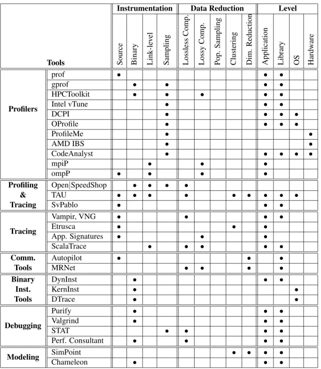
2.1 Comparison of techniques used in performance tools. . . 36

(15)

LIST OF FIGURES

1.1 Supercomputers: early and modern. . . 3

(a) ENIAC, 1946 . . . 3

(b) Cray 1, 1978 . . . 3

(c) IBM BlueGene/L, 2008 . . . 3

(d) Cray XT5 “Jaguar”, 2008 . . . 3

1.2 Concurrency levels of the top 100 supercomputers. . . 5

2.1 Computer system abstraction layers. . . 18

3.1 Multiscale decomposition for our levelL2-D wavelet transform . . . 59

3.2 Dynamic identification of effort regions. . . 64

3.3 Parallel compression architecture. . . 65

3.4 Data consolidation algorithm . . . 68

3.5 Tool overhead for Raptor and ParaDiS . . . 71

3.6 Compression and I/O times for 1024-timestep traces . . . 72

(a) Raptor on Blue Gene/L . . . 72

(b) ParaDiS on Blue Gene/L . . . 72

3.7 Blue Gene/P system architecture at Argonne National Laboratory . . . 73

3.8 Wavelet merge time for S3D on BG/P . . . 75

(a) Virtual-Node Mode . . . 75

(b) Dual Mode . . . 75

(c) SMP Mode . . . 75

3.9 Stand-alone merge performance, VN mode . . . 79

(16)

(b) 32 rows per process . . . 79

(c) 64 rows per process . . . 79

(d) 128 rows per process . . . 79

(e) 256 rows per process . . . 79

(f) 512 rows per process . . . 79

3.10 Stand-alone merge performance, dual mode . . . 80

(a) 16 rows per process . . . 80

3.11 Stand-alone merge performance, SMP mode . . . 81

(a) 16 rows per process . . . 81

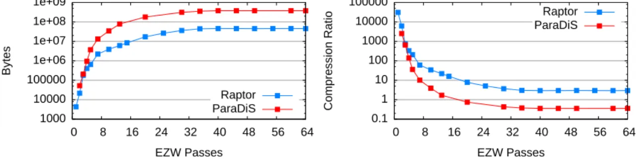
3.12 Varying EZW passes . . . 82

(a) Compressed size vs. encoded passes . . . 82

(b) Compression ratio vs. encoded passes . . . 82

3.13 Total data volume and compression ratios . . . 82

(a) Compression ratio vs. processes (Raptor) . . . 82

(b) Compression ratio vs. processes (ParaDiS) . . . 82

(17)

(d) Total compressed size vs. processes (ParaDiS) . . . 82

3.14 Embedding of the MPI rank space in S3D’s process topology . . . 83

3.15 S3D compressed data volume with standard and alternative topologies . . . . 84

(a) Data volume . . . 84

(b) Percent change with alternate topology . . . 84

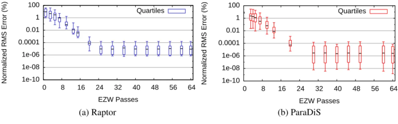
3.16 Error vs. encoded EZW passes . . . 85

(a) Raptor . . . 85

(b) ParaDiS . . . 85

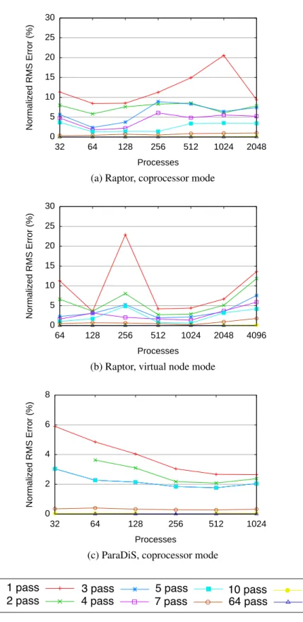
3.17 Median normalized RMS error vs. system size on BG/L . . . 86

(a) Raptor, coprocessor mode . . . 86

(b) Raptor, virtual node mode . . . 86

(c) ParaDiS, coprocessor mode . . . 86

3.18 Progressively refined reconstructions of the remesh phase in ParaDiS . . . 87

(a) 1 pass . . . 87

(b) 2 passes . . . 87

(c) 3 passes . . . 87

(d) 4 passes . . . 87

(e) 5 passes . . . 87

(f) 7 passes . . . 87

(g) 15 passes . . . 87

(h) Exact . . . 87

3.19 Exact and reconstructed effort plots for phases of ParaDiS . . . 90

(a) Force Computation, Exact . . . 90

(b) Force Computation, Reconstructed . . . 90

(c) Collision computation, Exact . . . 90

(18)

(e) Checkpoint, Exact . . . 90

(f) Checkpoint, Reconstructed . . . 90

(g) Remesh, Exact . . . 90

(h) Remesh, Reconstructed . . . 90

4.1 Minimum sample size vs. population size . . . 97

4.2 Run-time sampling in AMPL . . . 101

4.3 AMPL Software Architecture . . . 103

4.4 Update mechanisms in AMPL . . . 105

(a) Global . . . 105

(b) Subset . . . 105

4.5 AMPL configuration file . . . 106

4.6 Running sPPM with exhaustive monitoring . . . 110

(a) Timings. . . 110

(b) Data volume. . . 110

4.7 Mean (black) and sample mean (blue) traces for two seconds of a run of sPPM 112 4.8 AMPL trace overhead, varying confidence and error bounds . . . 113

(a) Percent execution time with TAU tracing . . . 113

(b) Percent execution time with effort tracing . . . 113

(c) Output data volume with TAU tracing . . . 113

(d) Output data volume with effort tracing . . . 113

4.9 Absolute and proportional sample size, varying system size . . . 119

(a) Data volume for ADCIRC on BlueGene/L . . . 119

(b) Data volume for Chombo on a Linux cluster . . . 119

(c) Data volume for ParaDiS on BlueGene/P . . . 119

(d) Data volume for S3D on BlueGene/P . . . 119

(19)

4.10 Data volume in stratified ADCIRC traces . . . 120

(a) Data overhead and average total sample size . . . 120

(b) Percent total execution time . . . 120

5.1 Structure of aggregated effort data. . . 126

5.2 Transposing Effort data. . . 127

5.3 Structure of coefficients after applications of the inverse wavelet transform . 135 (a) LevelLtransform . . . 135

(b) Level 3 approximation . . . 135

(c) Level 2 approximation . . . 135

(d) Level 1 approximation . . . 135

(e) Full reconstruction . . . 135

5.4 Modified EZW traversals for generating approximation matrices. . . 137

(a) Morton scan. . . 137

(b) Depth-first traversal. . . 137

5.5 On-line stratification framework. . . 141

5.6 Time and error in clustering effort regions with approximations. . . 144

(a) Time required to cluster approximations. . . 144

(b) Error compared to exhaustive data. . . 144

5.7 Using CLARA and PAM on effort data . . . 147

(a) Time for clustering operations, varying system size . . . 147

(b) Normalized error of CLARA vs. PAM . . . 147

5.8 Using wavelet approximations to cluster neighborhoods of points . . . 149

(a) Decompression time varying approximation level . . . 149

(b) Time to run CLARA varying approximation level . . . 149

5.9 Unified and stratified sample sizes for S3D . . . 151

(20)

(b) 2048 Processes . . . 151

(c) 4096 Processes . . . 151

(d) 8192 Processes . . . 151

(e) 16384 Processes . . . 151

5.10 Unified and stratified sample sizes for S3D using approximate data . . . 152

(a) 1024 Processes . . . 152

(b) 2048 Processes . . . 152

(c) 4096 Processes . . . 152

(d) 8192 Processes . . . 152

(e) 16384 Processes . . . 152

6.1 Libra software architecture . . . 156

6.2 Screenshot from a Libra client session. . . 160

6.3 Libra’s effort region browser . . . 161

6.4 Libra’s source viewer . . . 161

6.5 Most time-consuming call sites and load-balance plots for S3D . . . 162

(a) 4,096 processes . . . 162

(b) 8,192 processes . . . 162

(21)

LIST OF ABBREVIATIONS

AMPL Adaptive Monitoring and Profiling Library

API Application Programming Interface

BBV Basic Block Vector

BSP Bulk Synchronous Processing

CPU Central Processing Unit

DCT Discrete Cosine Transform

DCPI Digital Continuous Profiling Infrastructure

ENIAC Electronic Numerical Integrator and Computer

FFT Fast Fourier Transform

FPGA Field-Programmable Gate Array

GPU Graphics Processing Unit

GUI Graphical User Interface

HPM Hardware Performance Monitors

IBM International Business Machines Corporation

ILP Instruction Level Parallelism

I/O Input/Output

IP Internet Protocol

ISA Instruction Set Architecture

LINPACK Linear Algebra Package

LLNL Lawrence Livermore National Laboratory

LoF List of Figures

LoT List of Tables

(22)

MPI Message Passing Interface

MRNet Multicast-Reduction Network

NUMA Non-Uniform Memory Access

OS Operating System

OTF Open Trace Format

PAPI Performance API

PC Program Counter

PCA Principal Component Analysis

RAM Random Access Memory

RLE Run-Length Encoding

SIMD Single Instruction, Multiple Data

SISD Single Instruction, Single Data

SMP Symmetric Multiprocessing

SPMD Single Program, Multiple Data

SPRNG Simple Parallel Random Number Generator

STAT Stack Trace Analysis Tool

SWIG Simple Wrapper Interface Generator

SVD Singular Value Decomposition

TAU Tuning and Analysis Utilities

TCP Transmission Control Protocol

TLB Translation Lookaside Buffer

ToC Table of Contents

(23)

Chapter 1 Introduction

The first computers were created to solve mathematical problems faster and more accurately than humans. The Electronic Numerical Integrator and Computer (ENIAC), one of the ear-liest general-purpose programmable machines, was unveiled in 1946 and computed forty operations per second. This enabled engineers to calculate the trajectories of artillery shells thousands of times faster than was previously possible.

Today, predictive computer simulations are used to drive innovation and scientific discov-ery across a wide range of fields. Industrial designers use computer simulations to model the emissions of planes (Ball, 2008) and the mixing properties of shampoo (Spicka and Grald, 2004). Medical applications simulate blood flow and the behavior of cells (Pivkin et al., 2005; Pivkin et al., 2006; Richardson et al., 2008), and scientists simulate many natural phe-nomena, from weather systems (Michalakes, 2002) to quantum physics and the origins of the universe (on behalf of the USQCD Collaboration, 2008). The computing power required for any one these simulations dwarfs the simple computations performed on the ENIAC, and to-day’s fastest computers can compute over a quadrillion (1015_{) operations per second (Barker}

et al., 2008).

(24)

possible on 1946 hardware; the same calculation would have taken centuries. Increased performance also allows more detailed simulations, e.g., by increasing the resolution of a mesh, refining a model incrementally where needed, or running the simulation on a larger data set. This enables simulations to mirror reality more closely.

In this dissertation, we present techniques that can be used to measure and to improve the performance of scientific simulations. In particular, we focus on techniques for collecting and analyzing performance data from simulations on modern supercomputers that have large numbers of processors.

Tuning application performance for computer hardware has always been a painstaking and subtle process, but several factors of large-scale system design interact to make this more difficult today. In the following sections, we describe these factors in detail.

1.1 Evolution of Supercomputer Design

(25)

(a) ENIAC at the Army Ballistic Research Center, Maryland, 1946. (40 operations/sec.)

(b) Cray 1 at Lawrence Livermore National Laboratory, 1978. (8×107operations/sec.)

(c) IBM BlueGene/L at Lawrence Livermore Na-tional Laboratory, 2008. (4.78 × 1014

opera-tions/sec.)

(d) Cray XT5 “Jaguar” at Oak Ridge National Lab-oratory, 2008. (1015_{operations/sec.)}

(26)

Supercomputers have evolved since the vector era. Modern machines exploit parallelism at many levels. At a high level, they integrate large numbers of commodity processors so that multiple instances of a single program may operate on different parts of a partitioned prob-lem domain. This model of computation is called Single Program, Multiple Data (SPMD) parallelism (Darema-Rodgers et al., 1984; Darema, 2001). Within each processor, super-computers may also support vector instructions (Ramanathan, 2006). Alternately, they may employ a co-processor, such as a Graphics Processing Unit (GPU) or a Field-Programmable Gate Array (FPGA), that supports vector computation (Endo and Matsuoka, 2008). Today, these instructions are implemented using multiple functional units, and the execution of sep-arate operations within a vector instruction can proceed in parallel. This is called Single Instruction, Multiple Data (SIMD) (Flynn, 1972) parallelism. Within each operation, func-tional units themselves are pipelined. Finally, modern processors may support Instruction Level Parallelism (ILP), where instructions from a sequential stream are processed out of their original order, allowing more instructions to execute concurrently.

(27)

1 10 100 1000 10000 100000 1e+06

1992 1994 1996 1998 2000 2002 2004 2006 2008 2010

Number of Processors

Mean Max Min

Figure 1.2: Concurrency levels of the top 100 supercomputers (Meuer et al., 2009).

sufficient size for larger systems cannot be built affordably.

Scaling problems with large shared memories led to distributed-memory parallel com-puters. In distributed-memory systems, each processor has a local memory, but it is not instruction-accessible from other processors. Processes running on distributed memory sys-tems communicate by passing messages over a network. Syssys-tems built with this architecture have come to be calledclusters. They may be simple networks of commodity PCs connected by commodity network links, or thousands of sophisticated, custom-built processors with very fast, proprietary interconnects.

Clusters have been built with far more processors than can be attached to a single shared memory, and it is this scalability that has led to their widespread adoption. In 1998, fewer than 20 of the fastest 500 machines were clusters,1_{and as of November, 2007, 410 of the 500} fastest machines (82%) employed this architecture.

Figure 1.2 shows concurrency levels over time for the top 100 supercomputers since 1993. Cluster sizes have increased exponentially over the years, which has led to the creation of ex-tremely large systems. The largest distributed-memory system in 2000 had slightly fewer than 10,000 processors, but the largest in 2008, the International Business Machines Cor-1_{According to performance on on the Linear Algebra Package (LINPACK) (Dongarra, 1987) benchmark, as}

(28)

poration (IBM) Blue Gene/L system at Lawrence Livermore National Laboratory (LLNL) contains 212,992 processors, over twenty times as many. The current rate of growth is accel-erating, and systems with millions of processors are expected to emerge within the next five years.

1.2 Multicore Systems

The number of nodes in large clusters is not the only source of increased concurrency in mod-ern systems. Recent trends in the microprocessor industry have led to concurrency increases at the single-chip level, as well.

Gordon Moore first observed in 1965 that the transistors per unit area on processor dies roughly doubled every year:

The complexity for minimum component costs has increased at a rate of roughly a factor of two per year . . . Certainly over the short term this rate can be expected to continue, if not to increase. Over the longer term, the rate of increase is a bit more uncertain, although there is no reason to believe it will not remain nearly constant for at least 10 years. That means by 1975, the number of components per integrated circuit for minimum cost will be 65,000. I believe that such a large circuit can be built on a single wafer. (Moore, 1965)

Transistor counts have continued to increase at roughly the same rate since Moore’s observa-tion, and the trend is now commonly called Moore’s Law.

Until recently, hardware designers used the extra transistors to improve sequential per-formance by exploiting ILP. Clock speed has also increased, along with miniaturization of chip components. However, chipmakers have reached physical limitations on pipeline depth and power dissipation2_{, and the returns of sequential performance improvements have} dimin-2_{Technically, engineers have reached the limits of power dissipation acceptable}_{for consumer parts}_.

(29)

ished.

Additional transistors are now used to fit more independent processors, orcoreson a sin-gle chip, but this has several consequences for programmers. While Moore’s Law translated to improved sequential performance, few changes were required for old code to take advan-tage of new hardware, and application developers could expect the peak performance of their programs to double in speed every 18 months as microprocessors became faster. Multicore chips have the potential to provide similar speed improvements, but now programmers must engineer their code explicitly to take advantage of task-level parallelism.

Multicore consumer chips have ramifications for scientific application developers at the high end, as commodity technologies are typically used in the nodes of large clusters. Par-allel application developers now face clusters of multicore nodes communicating via shared memory among processors on the same node and through a fast interconnection network among nodes.

1.3 Challenges for Performance Tuning

Extreme concurrency poses serious challenges for developers tuning large-scale applications. The higher the number of concurrent tasks, the more difficult it is for programmers to exploit available parallelism.

1.3.1 Amdahl’s Law

Amdahl’s law (Amdahl, 1967) tells us the maximum overall speed improvement we can expect when part of an algorithm is improved. If we can speed up a percentageP of a system by a factor ofS, the expected speedup is:

1

(30)

The numerator here is the normalized running time of the original algorithm, and the denom-inator is the normalized running time of the modified algorithm.(1−P)gives us the running time of the unmodified portion of the original algorithm, andP/S is the expected running time of the improved fraction. For parallelization, we can rewrite this formula as follows:

1

(1−P) + P_N (1.2)

P now represents the percentage of the original algorithm to be parallelized, and N is the number of processors to be used, or the peak parallel speedup3_{. Clearly, no matter how large} N becomes, speedup is limited by the sequential component of the algorithm,(1−P). For example, if we can parallelize 96% of an algorithm, then we can expect it to speed up by no more than a factor of 25.

1.3.2 Single-node Performance Problems

Performance tuning is the process of making an application perform well for specific hard-ware. In large supercomputers, this can refer to problems either at the single node level, or it may refer to problems arising from inefficient interactions between processes. The full range of single-node performance problems is beyond the scope of this dissertation, but we give a brief overview of the main concerns here.

On a single node, performance is dictated by several factors. First, problems may arise if an application does not make efficient use of the local memory hierarchy. Modern machines make extensive use ofcaches(Hennessy and Patterson, 2006a): small, fast memories with faster instruction access time than main memory. If all of the data used by an algorithm does not fit into cache at once, the processor must access main memory more frequently, which can lead to significant slowdowns.

(31)

Second, applications must take advantage of the specific instructions available on local processors to achieve maximum performance. As mentioned, modern processors often sup-port vector instructions, and if algorithms can be structured so as to perform several similar operations at once, these may be fused into a smaller number of SIMD instructions. Alter-nately, processors may be able to issue many different types of instructions at the same time (ILP), and algorithms can be tailored to take advantage of this functionality (Hennessy and Patterson, 2006b).

Finally, in the presence of shared memory and multithreading, node-local performance may depend on the efficient synchronization of concurrent threads. This may depend strongly on the speed of the memory hierarchy if threads use in-memory locking.

1.3.3 Inter-node Communication

Inter-node performance problems in large clusters arise from inefficiencies in communication and synchronization among processes in parallel applications. Because modern clusters are

distributed-memory machines, they must employ interconnect fabrics to connect the

(32)

To develop distributed-memory parallel applications, application programmers do not have to deal with high-speed networking protocols directly. Instead, they typically use a li-brary to handle synchronization and message passing between processes. Currently, Message Passing Interface (MPI) (MPI Forum, 1994) is thede-factoparadigm for large-scale parallel computation, and it defines a set of operations for communication between two processes

(point-to-point communication) and among groups of processes (collective communication).

Programs written with MPI make wide use of synchronous constructs, per the Bulk Syn-chronous Processing (BSP) model of parallel computation (Valiant, 1990). In the BSP model, computation is organized into coarse-grained, alternating phases of computation and com-munication. In computational phases, there is little or no inter-process communication, and processes work on locally serial portions of a larger parallel problem. Once all processes have completed a computation phase, state is exchanged in bulk during a communication phase, and computation resumes.

The specifics of network operations are determined by the MPI implementor. Implemen-tations can be designed to exploit the host machine’s native network architecture, but a poor MPI implementation can be a source of serious performance problems in large-scale appli-cations. For example, even on a high-bandwidth InfiniBand network, an implementation of collective operations such as multicast must avoid congestion to achieve good perfor-mance (Kumar and Kale, 2004).

(33)

1.3.4 Load Imbalance

Harnessing the full power of a machine with millions of processors requires developers to balance computational load by dividing the problem domain into units of equal (or approxi-mately equal) amounts of work. Load balance is particularly important in synchronous sys-tems because all members of a group of processes must complete a unit of work before any process can continue. This implies that if one process takes more time to complete a particu-lar task, all others must wait for it. In particu-large systems, this may mean that a hundred thousand tasks or more must idle.

Depending on the application, eliminating load imbalance may be trivial or it may prove very difficult. Some problems are easily partitioned, and per-node behavior is static over the course of a full run. However, the behavior of many modern applications can change over time. For example, adaptive mesh refinement methods may increase the resolution of their grids on some processes but not on others (Greenough et al., 2003; Colella et al., 2003b), leading to more work for processes with refinement. Collisions between model elements and other infrequent events in the simulation domain may give rise to transient computation.

Many applications employ dynamic load-balancing schemes to redistribute work among processes at runtime, but these rely on precise data about the application’s work distribution. As machines scale, this type of information becomes more difficult to collect, and load-balance schemes may not scale efficiently.

1.3.5 Measurement

(34)

mentation, or modifications to source or binary code. By measuring, we modify the system we observe. If we do not measure carefully, we may perturb the system’s behavior signifi-cantly. Instrumentation code takes time to run and to record observations, and if it is executed too frequently, the application may take much longer to run.

On large distributed-memory systems, measurement tools need a mechanism to store ob-served performance data. The largest supercomputers increasingly use diskless nodes (Gara et al., 2005; Vetter et al., 2006), so there may be no local storage on which to archive ob-served data. Large machines typically are connected to a high-performance Input/Output (I/O) system, but compute nodes typically communicate with the I/O system through the same network used by applications. Perturbation becomes a problem when performance data transport interferes with an application’s communication.

(35)

1.4 Summary of Contributions

To exploit the full computational power of future parallel machines, detailed measurements are needed to guide design decisions around the obstacles outlined above. A system-wide approach to measurement and optimization is needed; tools must collect enough data to cap-ture the increasing complexities of on-node performance issues and to distribute work in a large system effectively, but not so much data that I/O and networks are saturated or that measurements are perturbed.

This dissertation details and evaluates novel techniques for measuring and analyzing per-formance data on large-scale supercomputers. We apply these techniques to large-scale sci-entific applications to illustrate their effectiveness, but the techniques themselves are more generally useful. Parallel compiler developers, run-time authors, and application developers alike may apply our monitoring techniques to understand and tune the performance of their software on large machines.

The key contributions of this dissertation are as follows:

Scalable Load-balance Measurement. We present a novel technique for collecting two di-mensional load-balance data in parallel applications across processes and over time. This method draws on wavelet analysis from signal processing to compress system-wide, time-varying load-balance data to manageable size. Results show that compres-sion time is nearly invariant with system size on current I/O systems.

(36)

re-duced by one to two orders of magnitude for the system sizes tested. We also show that clustering can stratify a heterogeneous set of nodes into homogenous groups, further reducing trace overhead.

Combined Approach We combine the wavelet-compression and sampling approaches to reduce load-balance monitoring overhead further. We use the data collected by our scalable load-balance tool to guide on-line stratification of processes into performance equivalence classes. We then use this information to reduce the sample size required to monitor an entire system using our sampled tracing techniques.

Libra: An Integrated Analysis Tool. We have integrated our monitoring techniques into a

set of runtime tools and a GUI client for application developers. We show how the data collected using our techniques can be used to diagnose a load-imbalance problem in a large-scale combustion simulation. We further show that mining data collected using Libra is feasible on a single-node system.

1.5 Organization of This Dissertation

The rest of this dissertation is organized as follows:

In Chapter 2, we give an overview of the fundamentals of performance measurement, and we outline a framework for understanding different types of measurement and different types of data. We then summarize previous work in performance measurement in the context of this framework, and we summarize the limitations of existing tools and techniques.

Chapter 6 describes Libra, a scalable load-balance analysis tool. Libra makes use of the

Effort Model to represent load-balance data. We present the Effort Model and describe its

notions of absolute units of progress toward application goals and variable units of effort

(37)

architecture and its components.

In Chapter 3, we give a detailed description of Libra’s system-wide load-balance mea-surement component. This component makes use of wavelet compression and is inspired by techniques drawn from imaging and signal processing. To motivate the approach, we give an introduction to wavelet analysis, and we show that the wavelet representation is particularly effective for storing effort model data. Finally, we detail results of using this data collection component to measure load-balance information for large-scale scientific applications. Re-sults show that the method can achieve two to three orders of magnitude of compression with modest error, and that the approach is scalable enough to measure very large systems.

In Chapter 4, we introduce techniques for sampled tracing, and we show how these can be used for parallel performance analysis. To motivate this technique, we ground our approach in statistical sampling theory, and we describe the scaling properties that uniquely suit it to large systems. We then describe the architecture of Libra’s sampling component, and we detail the results of using it with several large-scale applications. We also apply a technique calledstratified sampling, and we show that it can be used to further reduce trace overhead in a sampled system.

Chapter 5 combines the ideas in Chapters 3 and 4 to adaptively stratify a running ap-plication into performance equivalence classes. We use data from our wavelet compression technique with scalable clustering algorithms to show that clusters produced can be used to adaptively stratify traces on-line. We further show that dynamic stratification reduces the sample size required to monitor a large system by up to 60% over a unified sampling ap-proach.

(38)

Chapter 2 Background

2.1 Measurement and Optimization

Performance optimization is the process of making code run faster and more efficiently on a specific system implementation. Modern systems can be tremendously complex, and op-timization is difficult because it requires detailed knowledge of the components of these systems and how they interact. It is not always apparent where in a system a performance problem may lie, and detailed measurements are required to locate problemsbefore optimiza-tion is applied.

Choosing exactly what to measure requires that programmers understand the design of computer systems. Modern systems are organized into vertical layers ofabstraction. Each layer hides implementation details of the layer below and provides a simplified interface to the layer above. Programmers insert measurements at different levels in this hierarchy to measure different aspects of a system’s functionality, and this process is called instrumenta-tion.

Raw performance measurements can be copious, and to gain insight into application per-formance, programmers must compile these measurements into more concise performance

(39)

step to focus on key observations in the set of measurements. Depending on the type of characterization to be created, data reduction may involve discarding observations or it may simply transform the observations into a representation more amenable to analysis.

In this chapter, we detail fundamental techniques for performance measurement and char-acterization. To provide context,§2.2 describes the hierarchy ofabstraction layersfound in modern computer systems and the interfaces used to connect them.§2.4 details fundamental instrumentation techniques in the context of the abstraction hierarchy. We describe the types of performance characterizations that may be produced from such measurements in§2.5, and we detail generic techniques for data reduction in §2.6. Finally, §2.7 enumerates existing performance tools and describes how they implement the techniques described here.

2.2 Abstraction

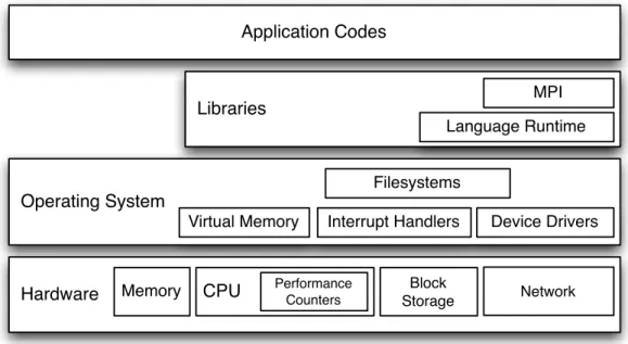
Modern computers are tremendously complex. The fastest microprocessors contain hundreds of millions of individual transistors (Bright et al., 2005), and the operating systems that run on them can contain millions of lines of code (Wheeler, 2002). Applications run on these operating systems can contain further millions of lines of code and may make use of libraries that contain millions more.

Integration at this scale is possible because software and hardware designers make exten-sive use ofabstraction: the process of factoring details from large problems and simplifying them into general concepts. Each piece in a large system has a well defined interface for its core behaviors, enabling other parts of the system to interact with it without concern for the details of its design.

(40)

Application Codes

Libraries

Language Runtime MPI

Hardware Block Network

Storage

CPU Performance _Counters Memory

Operating System

Filesystems

Device Drivers Interrupt Handlers

Virtual Memory

Figure 2.1: Computer system abstraction layers.

statically or dynamically, depending on the linkage mechanisms supported by the host Oper-ating System (OS).

Libraries and applications can interact with the host OS through system calls. To the user, system calls appear as ordinary functions, but beneath this abstraction they implement a control transfer from user code to the underlying OS kernel. The control transfer allows potentially unsafe operations to be encapsulated within the operating system, and prevents applications from interfering with each other. Operating systems usually provide an inter-mediary library to handle details of system call implementation; on UNIX-like operating systems, the C language runtime library handles this task.

System calls can incur more overhead than other library function calls, as the control transfer may require hardware interrupts and parameter data may need to be copied from user space to kernel space. This is not true of all machines. Some high-performance ma-chines (Gara et al., 2005) trade strict separation of memory between the OS and applications for performance.

(41)

in-cludes process control and managing access to shared hardware resources. Such resources are exposed to the user through abstractions. For example, when users make system calls to manipulate a local filesystem, the OS translates these calls to block storage commands and communicates with a disk drive on the caller’s behalf. Alternately, filesystem calls may be translated to network requests to access storage on a remote machine.

The operating system may allow users to register interrupt handlers to respond to asyn-chronous events. This enables applications to execute user code at a predetermined interval using a timer interrupt. On systems with more extensive hardware support, interrupt handlers may also be registered for performance-counter-related events.

2.3 Scalability

For large parallel scientific codes, the ability of an application to make efficient use of its interconnection network plays a large role in performance. Running a code on increasingly larger systems is calledscaling, and a code’s ability to communicate efficiently as the number of nodes in a system increases is referred to asscalability.

The scaling behavior of scientific applications is typically defined in terms of the relation-ship between the size of a computing system and the size of the problem on which it operates. In scientific simulations, the problem size is generally given as the number of model elements being simulated. For example, in a molecular dynamics simulation, the amount of compu-tation necessary to simulate a fixed amount of time depends on the number of molecules simulated. Alternately, a gas dynamics simulation might model a volume of gas as a dis-cretized mesh, in which case problem size is defined by the number of mesh elements in the simulation.

There are two primary scaling behaviors for parallel applications:

(42)

the problem size fixed. With ideal strong scaling, execution time will decrease propor-tionally to processor count as more processors are added to a system. Strong scaling inefficiencies arise when communication costs increase as more processors are added, or when model granularity is too small to allow even partitioning across all processes in the system. Amdahl’s law dictates that, in the limit, execution time will be dominated by the sequential components of computation in such systems.

Weak Scaling refers to increasing problem size proportionally with system size as more processors are added to a system. With perfect weak scaling, execution time remains constant as system size is increased. Adding more processors to a weak scaling system increases the problem size that can be calculated in the same amount of time. This is useful when more detail or more elements are needed to simulate large physical sys-tems accurately, as opposed to allowing fixed-size problems to be solved more quickly, as in strong scaling.

2.4 Instrumentation

Code or hardware added to a system to record measurements is calledinstrumentation. In-strumentation can be applied at any level of the abstraction hierarchy, depending on what is to be measured. This section discusses fundamental techniques for instrumentation and the trade-offs associated with each of them.

2.4.1 Hardware Instrumentation

(43)

low-level hardware events accurately. Most systems therefore include higher-resolution timing registers to measure tighter intervals in terms of elapsed CPU cycles. Depending on the access method, such interval timers can offer precision in the microsecond or nanosecond regime.

Depending on the system, more extensive hardware counters may be available. Many modern processors provide a configurable set of registers called Hardware Performance Mon-itors (HPM) that can record counts of hardware events. Events themselves are monitored through special detectors integrated into the processor itself. Inputs from detectors are multi-plexed and connected to registers, and users can configure the registers to count events such as memory references, cache misses, Translation Lookaside Buffer (TLB) misses, branch mispredictions, instructions and network operations.

2.4.2 Trace Instrumentation

To use hardware instrumentation, and to take measurements while a program is running, instructions for measurement must somehow be inserted into the control flow of a running system. One method of doing this is to insert instructions in the control flow of an application or library itself, so that those instructions will be performed in the course of the application’s normal execution. Instrumentation routines inserted this way may measure intervals with the timers described above, or they may simply record the occurrence of some software event. Such techniques are calledtracing.

Source Code Instrumentation

A straightforward way to make sure that instructions are executed at certain points in a pro-gram’s control flow is to insert calls to instrumentation routines directly into the source code and compile them along with the program itself. This is calledsource code implementation.

(44)

code when they add statements to output data to the screen or to a file. This allows program-mers to observe the order of events at runtime as they occur. However, inserting source code instrumentation by hand may be tedious if a large number of routines in a program are to be measured. In such cases, a parser may be used to insert calls to measurement routines into source code automatically. The modified source code then can be compiled and run to take measurements and to record events.

Source code instrumentation can be applied to any software, including applications, li-braries, and operating systems, provided that the source code is available. On some systems, instrumenting at lower levels of abstraction may be difficult, depending on what rights the user has on a system. For example, it may be difficult and time-consuming to instrument, re-compile, and install a new operating system on a production machine. Likewise, proprietary library source code may be unavailable to the end user.

Source code instrumentation is astatictechnique. When measurement code is compiled with an application, the application is perturbed slightly when the instrumentation is exe-cuted. The amount of perturbation depends on what specific actions the instrumentation performs and how frequently it is executed in the course of a run. Guard statements can be placed around instrumentation code to effect dynamic enablement and disablement of the ac-tual measurements. Even if instrumentation is disabled, guard statements still require a small amount of time to execute, so there is no way to avoid this probe effect completely.

Binary Instrumentation

Another technique for inserting instrumentation into a system’s control flow is to modify its object code. This is calledbinary instrumentation. Like source code instrumentation, binary instrumentation adds instructions that are executed along with those of the program.

(45)

Typically, an instruction at the beginning of an instrumentation point is replaced with an unconditional jump, which transfers control to special instrumentation code called a

trampo-line function. The trampoline then runs to completion and jumps back to just after the point

where control was diverted. Binary instrumentation may be performed statically before an executable runs, or it may be performed by modifying a running process’s memory through a debugger interface.

One advantage of binary instrumentation is that there is no probe effect when it is not enabled because the instrumentation is never executed. In addition, it can be applied to unmodified object code without recompiling, but the object code must be modifiable by the instrumentor. Thus, it may be impractical in production systems to instrument system code or kernel routines using this technique, but some operating systems support adding limited dynamic instrumentation to kernel routines.

Link-level Instrumentation

We have discussed techniques for inserting trace instrumentation by modifying source code, binaries, and running processes. A final mechanism for injecting instrumentation in an ap-plication’s control flow is to use the linker.

If an application makes use of a particular library, its calls to those libraries must be resolved by either a static linker or a dynamic loader. Programmers can make a custom library that implements wrappers for function calls of the measured library. If the application is linked with the modified library, its library calls will resolve to instrumentation routines, and the unmodified application code can run with an instrumented version of the library.

Link-levelinstrumentation is useful for measuring the interactions of an application with

(46)

after executing instrumentation.

Link-level instrumentation is convenient for the programmer in that it does not require that the measured application be recompiled. If only static linking is available, it is necessary

tore-linkan application. With dynamically linked libraries, this may not be necessary. Many

operating systems support for forcing an instrumentation library to be loaded at the start of runtime (e.g. via the LD PRELOAD environment variable in Linux). Loading a library at this point forces library calls to resolve to routines in the instrumentation library, even if the original library is also loaded.

2.4.3 Sampling

We have discussed several techniques for trace instrumentation. In addition to tracing, we may also elect to usesamplingto measure computer systems and applications.

Samplingis a form of asynchronous instrumentation. Instead of embedding instructions

directly into an application’s control flow, as in tracing, we take periodic measurements, or

samples,asynchronously. Depending on how samples are taken, they can be used determine

where an application is spending its time or where it consumes a particular resource.

Typically, sampling is implemented by registering interrupt handlers with the operating system. Most systems support periodic timer interrupts, where execution is interrupted at a regular interval over time. Depending on hardware support, there may be other, finer-grained interrupt mechanisms for tools to use. For example, many systems allow users to register interrupt handlers to be called after a certain number of CPU cycles. For systems with HPM counters, many systems also allow hardware counter interrupts, such that code can be sampled periodically according to instances of particular hardware events.

(47)

depending on the particular installation. For application and library code, however, at least timer interrupts are supported on most current platforms.

2.4.4 Trade-offs

Sampling and tracing are complementary techniques. Tracing allows the programmer to observe events as they happen at runtime, since instrumentation is embedded directly into a system’s control flow. This allows for more complete coverage. With trace instrumentation, an instrumented function is guaranteed to be observed each time control passes to it, and we know that the events recorded are exactly those that occurred at runtime. With sampling, there is no such guarantee.

Trace instrumentation can incur significant probe effects if the routines instrumented are executed frequently, which may make very fine-grained traces of applications cumbersome or infeasible. If a tight loop is instrumented with costly trace instrumentation, an application can take many times its original running time to finish, which may distort performance mea-surements. Some tools take a complementary approach and measure only particular routines so that trace instrumentation is sparse and the application is unperturbed.

The cost of sampling is a trade-off between overhead and sampling error. If the sampling rate is too low, infrequent events can escape observation. If the sampling rate is too high, an application can be perturbed severely. Typically, sampling tools take the middle ground here, using a sampling rate that incurs little overhead but still achieves reasonable code coverage.

2.5 Performance Characterization

(48)

selected guides the type of instrumentation used for measurement.

2.5.1 Profiling

Profiling is a technique used to map regions of source or object code to the amount of a partic-ular resource they consume. In the most common case, the resource measured is cumulative time, but profiles may also be generated from HPM measurements.

There are two general types of profiles. Flat profiles are direct mappings from static code regions to the time they consume. This type of mapping does not take dynamic calling context into account, so the time attributed to a particular region in a flat profile is the time spent in that region regardless of where it was called. Call-path profiles attribute time to particular calling contexts. This can be useful if selected functions are called from multiple places within an application. For example, if a given solver is used for two phases of a complex physics code, a call-path profile can provide insight into which context takes the most time to solve.

Both types of profiles may be generated either from trace measurements or from sam-pling. For a full call-path profile to be generated with trace instrumentation, all function entry and exit points must be instrumented. Excessive perturbation can result if some func-tions are called too frequently.

Sampling can be used to generate statistical call-path profiles if facilities are available to unwind a program’s call stack. This can be a costly operation, and in the presence of optimization (e.g., from compilers), it may be difficult or impossible to unwind the stack completely. Sampled flat profiles are simpler to generate in that they require only that the Program Counter (PC) be recorded.

(49)

PCs are mapped to statements in source code or to particular functions, giving a higher-level view of where a program spends its time. The granularity of profiles generated from trace data depends on the granularity of the trace instrumentation itself.

2.5.2 Tracing

Atraceis a performance characterization generated from observations of performance events

(e.g., those recorded by trace instrumentation) over time. Unlike profiles, which discard time information, a trace can capture the full sequence of events in a program’s execution.

Traces can be useful in determining evolutionary behavior in simulations. For example, model data in a parallel simulation may change significantly as the simulation progresses. After some time, more work may be required on some processes than others, and aggregating results over time may discard such potentially useful information. Likewise, traces can be useful for analyzing the correctness of a program’s execution, because they give a precise ordering of events. This is difficult with profiles, because timing information, and thus insight into causality, is discarded.

The added information present in traces comes at a price in terms of space. Whereas single-process profiles are relatively compact (their size is a function of static code size), traces grow with the length of a run. This can consume very large amounts of disk space.

2.5.3 Phased Profiling

Profiling and tracing are complementary techniques, and attempts have been made to com-bine them inphased profiling. Phased profiling records profiles for predefined time windows over the course of an application’s execution. This allows application developers to see the behavior of their applications evolve over time, yet it can consume considerably less space than a full trace, depending on the window size used.

(50)

has ended and that another has begun. Techniques have also been developed to detect phases in code automatically. These techniques use statistical analyses on performance metrics to differentiate the behavior of the code at different times during execution. Such tools have applications to performance monitoring for phased profile analysis. They also have been applied to the computer-architecture design process in the SimPoint (Perelman et al., 2006) tool. This tool is described in more detail in§2.7.7.

2.5.4 Performance Modeling

Profiles and traces are not the only forms of performance characterization, but they are two of the most widely used in the field of performance analysis. Other techniques have been developed topredictthe performance of future runs of applications based on historical data. This section describes some of these techniques.

Compile-time Scalability Analysis

Mendes and Reed (Mendes and Reed, 1998) present a methodology for assessing the scal-ability of applications based on information gathered at compile time. Specifically, they modified a Fortran D95 compiler (Adve et al., 1994; Wang et al., 1995) to convert all loops in a program to symbolic expressions in terms of problem size and number of processors. The compiler also gathers information on the instruction distribution within loops. Costs of in-structions as well as of send and receive operations are evaluated offline by machine-specific meta-benchmarks. A sum of loop send, receive, and instruction breakdowns weighted by these costs is used to predict upper and lower bounds for total program execution time.

(51)

dominate execution time. This information can guide performance engineers to places in the code that need optimization.

Convolution-based Performance Prediction

Snavely et al. demonstrate that application performance can be modeled locally by exam-ining memory hierarchy behavior, since the ability of a code to manage memory effectively dominates local performance (Snavely et al., 2001). However, modern architectures use in-creasingly complex hierarchies of caches, and it is unlikely that an application that has a certain memory performance on one architecture will have similar performance on another.

Snavely et al. use a benchmark to evaluate sustained load and store performance for a sin-gle processor with various memory access patterns. Based on the results of this benchmark, they create a mapping from access parameters to benchmark performance.

The authors then use a simulator to generate basic block profiles of scientific codes. The simulator can be configured to reflect the memory hierarchy of arbitrary architectures, and it gives cache-miss rates for each basic block in the simulated code.

Convolution is applied to combine the miss rate profile for basic blocks with the memory profile, and the result can be used to predict the execution time of applications. The authors profile sequential kernels from the NAS Parallel Benchmarks (NPB) (Bailey et al., 1991), and their method predicts execution times within 4% error. When extended to predict the time of parallel codes, it is accurate to within 20%.

(52)

2.6 Data Reduction

Because computer systems are complex, the space of potential performance measurements is large and many-dimensional. A single process can generate more data than is convenient for humans to digest, and a large parallel machine can produce far more than this.

Because of this complexity, we must be judicious in choosing the measurements that we take and in deciding how much data to record. Ideally, we would record just enough perfor-mance data to diagnose a problem, but we may not know on which processes or in which parts of a run a performance problem may arise. Recordingall available performance data can be impossible, as in the case of HPM counters, where not all values may be monitored at once; or impractical, as in the case of large traces, where disk space and data-mining capacity comes at a steep cost.

Performance tools make use of a variety of techniques for data reduction. In this section, we describe these techniques and the trade-offs involved in each.

2.6.1 Data Compression

Data compression is any technique that reduces the number ofbitsneeded to store informa-tion. Data converted to such a representation isencoded, and when it has been returned to its original representation, it isdecoded.

Lossless Compression

Lossless compression refers to compression after which the original representation can be

reconstructedexactly from the encoded representation. Lossless compression relies on the fact that most real-world data has at least some statistical redundancy.

(53)

on how compactly data can be represented using such techniques.

Entropy encodingis one of the most common forms of lossless compression. Two

exam-ples of entropy coding are Huffman coding (Huffman, 1952) and arithmetic coding (Rissanen and G. G. Langdon, 1979). These techniques both rely on the higher probability of encoun-tering some symbols than others in the input data. More frequently occurring input symbols are are represented with smaller output symbols and less frequently occurring symbols with larger output symbols, thus reducing the size of the representation.

Other lossless compression algorithms may use statistical models or dictionaries to record frequently occurring patterns in the input data. The simplest example of such an encoding is Run-Length Encoding (RLE), which stores contiguousrunsof a symbol in the input data as the symbol and an associated number of repetitions. Other encoding schemes use more so-phisticated dictionary lookup schemes, as in Lempel-Ziv-Welch (LZW) (Welch, 1984) cod-ing.

Lossy Compression

As mentioned, Shannon entropy bounds the compression that can be achieved if an input representation is to be compressed and then reconstructed exactly. However,lossy compres-sioncan allow for much greater reductions in data volume, if the user is willing to accept an approximate reconstruction of the original data.

(54)

Lossy compression techniques offer a trade-off between data volume and accuracy. The more data that an encoder writes to disk, the more closely the output representation can be reconstructed to mirror the original inputs, and vice versa. Users of lossy compression schemes can typically set acompression levelto control the trade-off.

Lossy techniques have been applied widely to process image, video, and audio signal data. The popular JPEG image compression format, the MPEG video compression format, and the MP3 audio compression format all use a Discrete Cosine Transform (DCT) coupled with lossy encoding to reduce the size of media files significantly. Similarly, the JPEG-2000 (Adams, 2002) image format uses a discrete wavelet transform coupled with lossy coding techniques.

Lossy compression also may be employed for performance tracing. Lu and Reed present

theapplication signature (Lu and Reed, 2002), a technique that represents numerical trace

data concisely. Given a time-ordered sequence of metric values gathered at runtime, its signature is a piecewise-polynomial approximation of this sequence.

Signatures are constructed dynamically, and programmers can adjust an error threshold to modulate recorded trace size. Larger error thresholds will cause the fitting algorithm to generate a more compact signature at the expense of accuracy. Likewise, smaller error thresholds lead to larger, more accurate signatures. An exhaustive trace is a signature with error threshold of zero.

(55)

2.6.2 Population Sampling

Population sampling is a technique for estimating the behavior of a set by observing only

a fraction, or sample, of its elements. Traditionally used in polling and survey research, sampling is useful because it can reduce the cost of data collection significantly if collecting observations is expensive. Because it reduces the number of observations that need to be made, sampling is also useful for reducing data volume.

The minimum sample size for a population with constant variance scales more slowly than the population itself, allowing one to sample comparatively small numbers of nodes for accurate estimates of very large populations. Notably, forN monitored processes, fixed error boundd, and desired deviations from the estimator meanzα, a sample size ofnis required,

wherensatisfies:

n ≥N

"

1 +N

d zαS

2#−1

(2.1)

Typically, confidence and accuracy of sample surveys are computed after the survey is complete, from the size of the sample taken. Equation 2.1 can be applied to reverse this process. The user specifies desired confidence and error bounds, and the required minimum sample size for meeting these bounds is computed. The user then has a probabilistic guar-antee that his estimation will be accurate. Furthermore, sampling scales very well to large quantities of nodes. Note that as N increases, n approaches (zαS/d)2. This implies that

sample size is proportionally smaller for very large numbers of processes.

(56)

8% error while only sampling 1.5% of the total number of machines.

Since collected data volume is proportional to the number of processes, this technique can reduce monitoring overhead in large clusters substantially.

2.6.3 Cluster Analysis

Cluster analysisrefers to a number of statistical algorithms for finding homogeneous groups,

or clusters, within data. Like other techniques described here, clustering relies heavily on

statistical redundancy in input data. While typically not described as a data reduction tech-niqueper se, clustering can be useful for data reduction because it allows large data sets to be described in terms of a smaller number of clusters.

Two widely used techniques for clustering arehierarchical, oragglomerative, clustering algorithms (Kaufman and Rousseeuw, 2005a), andpartitionalclustering algorithms (Kauf-man and Rousseeuw, 2005b; Kauf(Kauf-man and Rousseeuw, 2005c; Forgy, 1965; Hartigan and Wong, 1979; Lloyd, 1982). Users of both of these algorithms define adistance measureon the input data, which is used by the algorithms to determine the similarity of pairs of objects in the input data. In hierarchical clustering algorithms, groups of objects are merged recur-sively, producing a hierarchical tree of clusters with increasing granularity. In partitioning algorithms, the number of clusters,k, is specified in advance, and the algorithm attempts to find a group that fully or nearly minimizes the distance between objects in k clusters. We describe techniques for cluster analysis in more detail in§5.2.2.

Scalable performance measurement and analysis