STATISTICAL METHODS FOR CORRELATED DATA FROM OBSERVATIONAL STUDIES
Hongtao Zhang
A dissertation submitted to the faculty of the University of North Carolina at Chapel Hill in partial fulfillment of the requirements for the degree of Doctor of Philosophy in the
Department of Biostatistics.
Chapel Hill 2015
c
2015
ABSTRACT
Hongtao Zhang: Statistical Methods for Correlated Data From Observational Studies (Under the direction of Jianwen Cai and Haibo Zhou)
First, we consider case-cohort studies with multiple disease outcomes. To investigate the effect of a risk factor on different diseases, multiple case-cohort studies are usually conducted. To compare the effect of a risk factor on different types of diseases, times to different disease events need to be modeled simultaneously. Existing case-cohort es-timators for multiple disease outcomes utilize only the relevant covariate information in cases and subcohort controls, though many covariates are measured for everyone in the full cohort. Intuitively, making full use of the relevant covariate information can improve efficiency. To this end, we consider a class of doubly-weighted estimators for both regular and generalized case-cohort studies with multiple disease outcomes. The asymptotic prop-erties of the proposed estimators are derived and our simulation studies show that a gain in efficiency can be achieved with a properly chosen weight function. We illustrate the proposed method with a data set from Atherosclerosis Risk in Communities (ARIC) study. Second, we investigate marginal structural Cox model for clusters of correlated failure time observations. In many studies, subjects in the same community form natural clusters and are thus correlated. We formulate marginal structural Cox model for this type of data and prove the consistency and asymptotic normality of the estimator. Simulation studies show that marginal structural Cox model perform properly by yielding unbiased estimate and satisfactory confidence interval coverage. The proposed method is implemented using a claim data assessing the effectiveness of INSPIRIS home visiting health care program.
TABLE OF CONTENTS
CHAPTER 1: INTRODUCTION . . . 1
CHAPTER 2: LITERATURE REVIEW . . . 5
2.1 Marginal Structural Cox Model . . . 5
2.1.1 Cox Model and Extension to Multivariate Case . . . 5
2.1.2 Marginal Structural Cox Model . . . 7
2.2 Statistical Methods for Biased Sampling Designs . . . 9
2.3 Statistical Methods for Case-cohort Design . . . 16
2.3.1 Univariate Case-cohort Design . . . 16
2.3.2 Multivariate Case-cohort Design . . . 27
CHAPTER 3: MORE EFFICIENT CASE-COHORT ESTIMATORS . . . 33
3.1 Introduction . . . 33
3.2 Model and Estimation . . . 35
3.2.1 Notations and Model Definition . . . 35
3.2.2 Estimation . . . 36
3.3 Asymptotic Properties of General Doubly Weighted Estimator . . . 40
3.3.1 Asymptotic Results . . . 40
3.3.2 Generalization to Arbitrary Second Level Weight . . . 43
3.3.3 Generalization to Stratified Sampling Design . . . 44
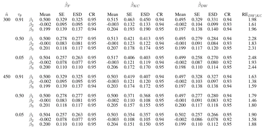
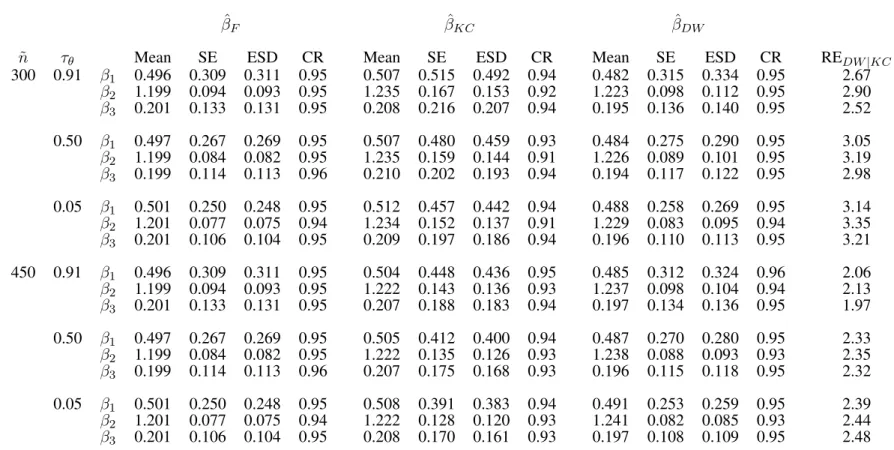
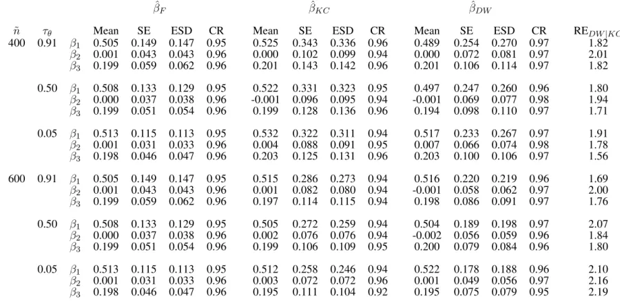
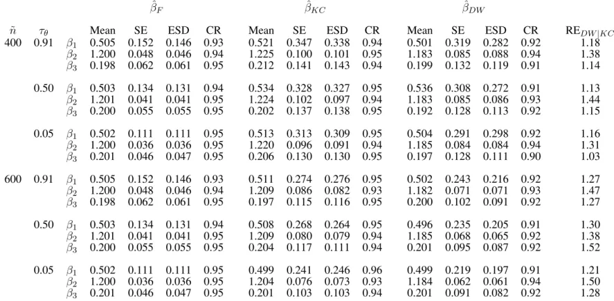
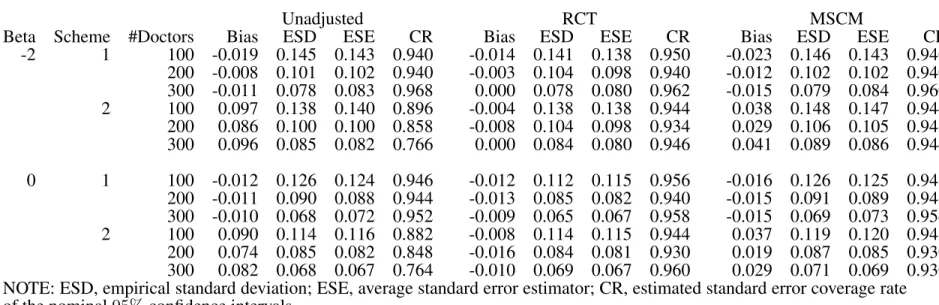
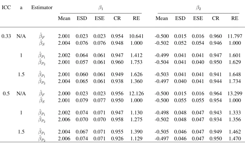
3.4 Simulation Studies . . . 46
3.4.1 Traditional Case-cohort Design . . . 47
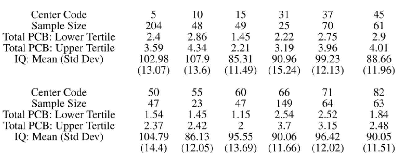
3.5 Data Analysis . . . 49
3.6 Concluding Remarks . . . 51
3.7 Explicit Form ofDDW(β) . . . 52
3.8 Proof of Theorem 3.3.1 . . . 53
CHAPTER 4: MSCM FOR CLUSTERED FAILURE TIMES . . . 73
4.1 Introduction . . . 73
4.2 Statistical Framework . . . 76
4.3 Estimation and Inference . . . 77
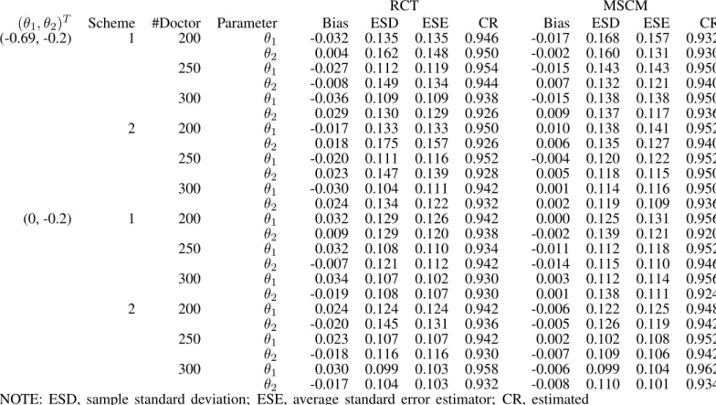
4.4 Simulation . . . 90
4.4.1 Covariates and Correlated Failure Time . . . 90
4.4.2 Binary Time-independent Treatment . . . 92
4.4.3 Primary Treatment, with a Possibility of Secondary Treatment . . 95
4.5 Data Analysis . . . 98
4.6 Discussion . . . 100
CHAPTER 5: MIXED EFFECT MODEL FOR CLUSTER-BASED PDS . . . 105
5.1 Introduction . . . 105
5.2 Design and Semiparametric Inference . . . 108
5.2.1 Design and Data Structure . . . 108
5.2.2 Estimation and Asymptotic Results . . . 109
5.3 Simulation . . . 114
5.4 CPP Data Analysis . . . 116
5.5 Discussion . . . 118
5.6 Proof of Theorems . . . 119
CHAPTER 6: SUMMARY AND FUTURE RESEARCH . . . 130
CHAPTER 1: INTRODUCTION
In medical studies, multivariate data may occur on various occasions. For example, one subject may experience multiple outcomes of interest. On the other hand, subjects sharing similar characteristics can form intrinsically correlated clusters. Proper methods are needed to analyze such data. This dissertation concentrates on multivariate statistical methods in observation studies, possibly with biased sampling schemes.
Using Full Cohort Information to Improve the Efficiency of Multivariate Marginal Hazard Model for Case-Cohort Studies
As all studies are conducted with a limited budget, the maximum study sizes are often restricted by the cost of the exposure ascertainment. Cost-effective sampling designs have long been desired and play an important role in success of many biological studies.
of the first-phase covariate data. For example, the Atherosclerosis Risk in Communities (ARIC) study is a large cohort study that involves 15,792 participants. One important aim of ARIC study was to assess lipoprotein-associated phospholipase A2(Lp-PLA2) as poten-tial risk factor of atherosclerosis and its sequelae, so that physicians may consider making Lp-PLA2 a complementary risk factor beyond the traditional ones. Given the large cohort size and funding limitation, measuring Lp-PLA2 in labs for all the participants would be infeasible. Alternatively, case-cohort studies were carried out: Lp-PLA2 were obtained only for patients suffering cardiovascular heart disease (CHD) or stroke, together with a random subcohort that were event-free. Investigators (Ballantyne et al. 2004, 2005) stud-ied candidate biomarkers of inflammation as possible risk factors. However, the first-phase covariate information such as LDL/HDL cholesterol level was not fully utilized. Another feature of ARIC study is that multiple disease (e.g CHD and incident stroke) outcomes were monitored simultaneously. Kang and Cai (2009) proposed a weighted estimating equation approach to fit a marginal proportional hazard model with multiple diseases. Kim et al. (2013) used a modified weight function that was empirically shown to improve the ef-ficiency over Kang and Cai (2009) model. In the first topic, we consider a doubly-weighted approach that utilizes all covariate information to improve the efficiency.
Marginal Structural Cox Models
Randomized clinical trials are generally considered the ‘gold standard’ in establishing causal relationship due to its ability to balance distributions of subject characteristics across treatment groups. Since the treatment assignment is not confounded with the patient’s baseline characteristics, treatment effect can be estimated simply by comparing outcomes between treated and untreated groups.
be-tween exposure and outcome. One major challenge in analyzing data from observational studies is confounding by indication, which is introduced if prognostic factor(s) can be re-lated to both treatment history and outcome. Recent years have seen increasing interests in observational comparative effective research (CER), mainly due to the growing adoption of electronic medical record (EMR) database.
Mixed Effect Model for Probability-dependent Sampling Design
There are numerous situations where the outcome of interest is measured continuously. Outcome-dependent sampling (ODS) scheme (Zhou et al. 2002, Weaver and Zhou 2005) was a two-stage sampling procedure proposed to obtain a more informative sample by over-represent the two distributional tails ofX, the exposure that is expensive to ascertain. ODS design is a popular choice for studies that values of outcomeY are known for all subjects, but the exposure variableXmay be expensive or difficult to ascertain. The data structure of the ODS sample consists of a first-phase simple random sample (SRS) and a second-phase simple random sample from two tails ofY. ODS scheme is useful when the investigators have some knowledge about the relationship betweenY and X. For example, ifY has a linear relationship withX, subjects sampled from two tails ofY distribution are more likely to have X-value that falls in its two distributional tails. However, such prior knowledge is not always feasible. To this end, probability-dependent sampling (PDS) scheme (Zhou et al. 2014) allows investigators to over-sample the two tails of X distribution without having knowledge ofX in advance. In some studies, e.g. Collaborative Perinatal Project, participants in the same clinic form natural clusters and are potentially correlated. The third topic of this dissertation is to extend PDS design to cluster-based studies.
CHAPTER 2: LITERATURE REVIEW
2.1. Marginal Structural Cox Model
2.1.1 Cox Model and Extension to Multivariate Case
Cox proportional hazard model (Cox 1972) is the most popular class of model used to analyze time-to-event data. For n independent subjects, the Cox model can be expressed as:
λ(t) = λ0(t)exp{βTX(t)},
where λ0(t) is the unspecified nonparametric baseline hazard function and β is the un-known parameters associated with the vector of possibly time-dependent covariatesX(t). Estimation of Cox model is based on partial likelihood (Cox 1975). The maximum partial likelihood estimate (MPLE)β, maximizes the partial likelihood functionˆ
L(β) = n
Y
i=1 Y
t≥0
{ e
βTXi(t) Pn
j=1Yj(t)eβ
TXi(t)} ∆Ni(t)
,
where Y(t) is the at-risk process and ∆Ni(t) = 1 if the ith subject has event of
inter-est (fails) at time t and 0 otherwise. Andersen and Gill (1982) investigated the asymp-totic properties of MPLEβˆusing martingale theory. Under mild regularity conditions, the MPLEβˆis consistent for the true parameterβ0and is asymptotically normal
n1/2( ˆβ−β0)→d N(0,I1(β0)−1),
In many studies, subjects may be intrinsically correlated. For example, patients that are treated in the same medical clinic form clusters and are likely to be correlated. Another example is that multiple diseases may be monitored simultaneously for one subject. Either example leads to the multivariate survival analysis scenario. Currently, there are in general two classes of models to analyze multivariate time-to-event data. One class is known as the frailty models (Hougaard 1995). We use subscriptk = 1, . . . , K to index the clusters andi = 1, . . . , n0 to index patients or observations within a cluster. Frailty models have the form
λki(t|Qk) =Qkλ0(t)exp{βTXki(t)},
in which the cluster-specific random effectQk is assumed to follow a known distribution.
Qk resembles a random effect in linear mixed effect models and it is commonly assumed
to follow Gamma distribution (Clayton and Cuzick 1985) or positive stable distribution (Hougaard 1986).
The other class is the marginal models. Marginal models leaves the nature of depen-dence structure completely unspecified, rendering them more robust. Marginal models are usually of greater interest when the dependence structure is not of interest. Wei et al. (1989) suggested fitting a marginal Cox proportional hazard model that can be formulated as
λki(t) =λ0k(t)exp{βkTXki(t)}. (2.1)
Each cluster k has a distinct baseline hazard function, which suits well with the multi-ple disease situation. Model (2.1) can be immulti-plemented using standard software packages. Asymptotic results also confirm that the MPLE is a consistent estimator whose variance can be approximated by a robust estimator that is in the sandwich form.
hazard function across all clusters:
λki(t) = λ0(t)exp{βTXki(t)}. (2.2)
The asymptotic results were similar to those of model (2.1).
2.1.2 Marginal Structural Cox Model
Marginal structural models (Robins et al. 2000, Hernan et al. 2001) are a class of mod-els used in causal inference. Such modmod-els handle the issue of time-dependent confounding in evaluation of the efficacy of interventions by inverse probability weighting for receipt of treatment. Marginal structural Cox model (Hernan et al. 2000) for time-to-event data is an important extension. It takes a form that resembles the regular Cox model, but is formulated using counterfactual arguments. Consider an observational study where the outcome of interest is survival time T. Let A(t) indicate the observed treatment(s) re-ceived which can take various forms. For example, it could be an indicator of treatment initiated at baseline, an arbitrary function of dose level, or a time-dependent indicator of treatment received at time t. Let L(t) denote a vector of covariates and L(0) repre-sents baseline covariates. Use overbars to represent history up to timet (tincluded) such that A(t) = {A(u) : 0 ≤ u ≤ t}. L(t) is defined analogously. Let a be any treat-ment, potentially contrary to what was observed, that a subject could receive. Specifically, a ={a(t) : 0≤ t ≤ τ}, where τ is the duration of the study. Observed treatment history A(t) can be considered a particular realization of a(t). There will be a failure time Ta
We need the following three assumptions that are needed for marginal structural models
Assumption 2.1.1. T =Tafor anyasuch thata(t) =A(t), t≤T
Assumption 2.1.2. pr(A(t)|A(t−), L(t−))>0, for anyt ∈[0, τ]such that
pr(A(t−), L(t−))>0
Assumption 2.1.3. Ta ⊥⊥A(t)|A(t−), L(t−), for anya
Assumptions 2.1.1 and 2.1.2 are usually referred to as consistency and positivity as-sumptions, respectively (Hernan and Robins 2006, Cole and Frangakis 2009). Assumption 2.1.1 states that an individual’s observed failure time T is precisely the potential failure timeTaunder a certain observed exposure historya. Assumption 2.1.2 states that the
prob-ability of receiving any particular treatment at timet, given treatment and covariate history up to t, is greater than zero. Assumption 2.1.3 is known as no unmeasured confounding (Hernan et al. 2000). In practice, only assumption 2.1.2 is testable.
We consider the marginal structural Cox model for the hazard of failure at timet had the subject received treatmenta
λTa(t) = λ0(t)exp{β
T
0a(t)}, (2.3)
whereλ0(t)is an unspecified baseline hazard function and β0 is the unknown parameter vector. exp{β0}will have the interpretation of average treatment hazard ratio.
Estimation of parameters in model (2.3) is carried out via inverse probability weighting technique. Before proceeding to likelihood, we need to discretize the study duration[0, τ]
so that weight functions can be defined. Let0≤t1 < t2 <· · ·< tD ≤τbeDdistinct time
visits. Define
W(t) = Y td≤t
1
pr[A(td)|A(t−d), L(td)]
. (2.4)
At any given time t, the subject is inversely weighted by the probability of receiving the observed history of treatment up to that moment. By inverse probability weighting, we create a hypothetical pseudo-population whereL(t)⊥⊥A(t)|A(t−)holds at timet.
When L(t) contains confounders that are strongly correlated to treatment A(t), the estimate weight Wˆ(t) can vary drastically, resulting in high sampling variability in βˆW.
As a remedy, Robins et al. (2000) and Hernan et al. (2000) suggested using a stabilized version ofW(t)
w(t) = Y td≤t
pr[A(td)|A(t−d)]
pr[A(td)|A(t−d), L(td)]
. (2.5)
In (2.5), the excessive contribution of W(t) can be offset by the probability conditional on treatment history solely on the numerator. Using either W(t)or w(t) will result in a weighted partial likelihood function that can be maximized using Newton-Raphson itera-tive algorithm. In her dissertation, Lee (2013) proved the asymptotic properties of marginal structural Cox model for the case-cohort design when subjects are independent.
2.2. Statistical Methods for Biased Sampling Designs
response is intrinsically binary, case-control designs (Prentice and Pyke 1979) are often preferred. The idea of case-control design is to over-sample cases that are believed to be more informative. Ordinary analysis can then be performed on the case-control sample.
On the other hand, there are numerous situations where the outcome of interest is measured continuously. Case-control design cannot be naturally extended to continu-ous outcome setting. In practice, investigators often dichotomize the outcome based on whether the outcome is above or below a certain cutoff (potentially subjective). How-ever, it is obvious that doing so will discard the information in the continuous outcome. Also, the results may be sensitive to the choice of cutoff. Zhou et al. (2002) proposed an outcome-dependent sampling (ODS) scheme to address this issue. To fix notation, let Y denote the continuous outcome variable andX the vector of covariates. Assume that Y can be partitioned intoK mutually exclusive and exhaustive strata by known constants −∞ = a0 < a1 < · · · < aK−1 < aK = ∞ and let the kth stratum be represented
by Ck = (ak−1, ak], k = 1, . . . , K. The data structure of the ODS sample consists of
an overall simple random sample (SRS) of size n0 and a simple random sample of size n1, . . . , nK from each of the K strata. The latter is referred to as ‘supplemental sample’.
Let nV = PKk=0nk be the total size of the ODS sample and N be the sample size in
the population. Borrowing terms from the measurement error literature, we refer to the ODS sample as the ‘validation sample’, and refer to the restnV¯ = N −nV observation
as the non-validation sample. LetV represent the index set of all observations in the val-idation sample, and letV¯ represent the index set of all observations in the non-validation sample. Their corresponding partitions Vk and V¯k are also defined. Although response
Y is observed for all observations, complete covariate information X is measured only in the validation sample. Zhou et al. (2002) utilized only the validation sample. Let GX
F(u) =pr(Y ≤u)andF(u|x) = pr(Y ≤u|x). Then the validation sample likelihood is
L(β, GX) =
n0 Y
i=1
fβ(y0i|x0i)gX(x0i)
× K Y k=1 nk Y j=1
fβ(ykj, xkj|ykj ∈Ck)
=
n0 Y
i=1
fβ(y0i|x0i)× K Y k=1 nk Y j=1
fβ(ykj|xkj)
F(ak|xkj)−F(ak−1|xkj)
× n0
Y
i=1
gX(x0i)× K Y k=1 nk Y j=1
gX(xkj)[F(ak|xkj)−F(ak−1|xkj)]
F(ak)−F(ak−1)
=L1(β)×L2(β, GX). (2.6)
The second component in (2.6), L2(β, GX), is a function of β because the
condi-tional distribution function F(·|x) depends upon β. Without specifying GX, inference
about β can be obtained by maximizing L1(β) with respect to β. Zhou et al. (2002) elected to leaveGX unspecified, making it an infinite-dimension nuisance parameter, and
used Lagrange multiplier arguments to derive a semiparametric empirical likelihood func-tion. Their discussion focused on partitioning Y into 3 strata and over-sample its two tails C1, C3. They profiled L2(β, GX) by fixing β and obtaining the empirical
likeli-hood function ofGX over all distributions whose support contains the observedX values.
During the process, four more parameters were introduced η = (π1, π3, ν1, ν3)T where π1 =F(a1), π3 = ¯F(a3) = 1−F(a3)andν1, ν3 were Lagrange multipliers. The param-eter estimator forθ = (βT, ηT)T can be obtained iteratively via Newton-Raphson method
and its asymptotic properties were derived.
Weaver and Zhou (2005) made attempt to utilize the information in the non-validation sample. It was assumed that, in addition to the complete observations in the ODS, in-formation regarding stratum membership would be retained for the observations in the non-validation sample. Clearly, this assumption would be satisfied as long as continuous responseY is measured for allN observations. LetfY(Yj;β) =
R
the unspecified marginal density ofY. The full sample likelihood is proportional to
LF(β, GX) =
Y
i∈V
fβ(Yi|Xi)
×
Y
i∈V
dGX(Xi)
×
Y
j∈V¯
fY(Yj;β)
. (2.7)
Denote the number of observations in the SRS that belong to the kth stratum asn0,k.
Nkis defined likewise for the population. Weaver and Zhou (2005) proposed to substitute
the unspecifiedGX with its consistent empirical estimator, that is,
ˆ
GX(x) = K
X
k=1 Nk
N Gˆk(x),whereGˆk(x) = X
i∈Vk
I{Xi ≤x}
nk+n0,k
.
The resultant unbiased estimator forfY(Yj;β)is then
ˆ
fY(Yj;β) = K
X
k=1
Nk
N(nk+n0,k)
X
i∈Vk
fβ(Yj|Xi). (2.8)
Substituting (2.8) into (2.7) and applying the log-transformation, one can obtain the estimated log-likelihood
ˆ
lF(β) =
X
i∈V
logfβ(Yi|Xi)
+
X
j∈V¯
log
K
X
k=1
Nk
N(nk+n0,k)
X
i∈Vk
fβ(Yj|Xi)
.
Consistent estimator is again found using Newton-Raphson method.
W provides no additional information about Y when X and Z are known. Zhou et al. (2011b) considered an outcome-auxiliary-dependent sampling (OADS) scheme. In addi-tion to theK partitions ofY, assume thatW can be partitioned intoJ mutually exclusive and exhaustive strata by known constants −∞ = b0 < b1 < · · · < bJ−1 < bJ = ∞
and let thejth stratum be represented by Bj = (bj−1, bj], j = 1, . . . , J. Then the
popula-tion can be partipopula-tioned into T = K ×J strata on the domain of Y ×W. For notational simplicity, use ∆t, t = 1, . . . , T to denote the strata. V,V¯ and corresponding partitions
Vt,V¯tare defined analogously. The outcome-auxiliary-dependent sample also consists of
two components: an overall SRS and a supplemental sample of size nt fromtth stratum.
These two components make up the validation sample, whose complement is referred to as non-validation sample. Using similar arguments as in Weaver and Zhou (2005), the full sample with likelihood
LF(β) =
T Y
t=0 Y
i∈Vt
fβ(Yi|Zi, Xi)dG(Xi|Zi, Wi)
× T
Y
t=0 Y
i∈V¯t Z
X
fβ(Yi|Zi, x)dG(x|Zi, Wi)
. (2.9)
G(X|Z, W) is again estimated non-parametrically. Let S denote thed−dimensional information components of(Z, W)in the sense thatG(X|Z, W) = G(X|S)almost surely. Zhou et al. (2011b) proposed to estimateG(x|s)via kernel smoothing. Specifically,
ˆ
G(x|s) = T
X
t=1
ˆ
πt(s) ˆGt(x|s),
where
ˆ
πt(s) =
PN
i=1I{(Yi, Wi)∈∆t}φh(Si−s) PN
i=1φh(Si−s)
,Gˆt(x|s) =
P
i∈VtI{Xi ≤xφh(Si−s)} P
φh(·)here is ad−dimensional kernel function with bandwidthh. SubstitutingGˆ(x|s)into
(2.9) to obtain the estimated likelihood function, then one can employ Newton-Raphson method to obtain the estimate ofβand consequently make inferences. In some studies, ob-servations may be intrinsically clustered (e.g. within medical clinics) and statistical meth-ods need to account for the cluster-level random effect. Xu and Zhou (2012) investigated cluster-based OADS. They postulated a linear mixed effect model forfβ(y|x, z)
Ymti =β0+β1Xmti+β2Zmti+um+emti (2.10)
The additional subscriptm = 1, . . . , M indexes the clusters. um ∼ N(0, σ2u), emti ∼
N(0, σ2) andu
m ⊥⊥ emti. Their likelihood function had a similar form as in Zhou et al.
(2011b). However, numerical integration technique was implemented to address the com-plexity introduced by the cluster-level random effectum. Wang and Zhou (2010)
consid-ered the OADS design with categorical response variable. Estimation and inference were carried out based on an estimated likelihood function.
So far in this section, the mean model linking the response to the exposure of interestX and covariatesZ was assumed to be linear. Specifically, the linear model isE(Y|X, Z) =
βTX +γTZ, whereβ and γ are unknown regression parameters. In many studies, it is
Recently, a probability-dependent sampling (PDS) scheme has been proposed (Zhou et al. 2014). Assume that the domain of the exposureXis partitioned into three mutually exclusive intervals: (−∞, xL]∪ (xL, xU]∪(xU,∞). Like ODS, an SRS is drawn from
the population at the first stage. Before supplemental sampling, a model forE(X|Y, Z)is fitted using the first-phase SRS. On the basis of this model, the chances of a new subject’s X conditional onY = y andZ = z, will be in (−∞, xL]and (xU,∞)are predicted by
ˆ
φ1(y, z) = ˆpr(X < xL|Y, Z)andφˆ3(y, z) = ˆpr(X > xU|Y, Z)respectively. Then
supple-mental samples are drawn from those whoseX are more likely to fall on the distributional tails ofX. For example, random samples can be drawn from those withφˆ1(y, z) > c1 or withφˆ3(y, z) > c3, wherec1 andc3 are thresholds. Assume thatfβ(y|x, z)has the linear
form
Y =β0+β1X+β2Z+e,
whereeis normal random error. LetG(X, Z)andg(X, Z)denote the joint CDF and PDF of(X, Z). Define
πk=pr{φk(Y, Z)≥ck} =
Z Z Z
fβ(Y|X, Z)g(X, Z)I{(Y, Z) :φk(Y, Z)≥ck}dY dXdZ.
The log-likelihood for the validation sample is
l(β,{pi}, π1, π3) =
X
i∈V
logfβ(Yi|Xi, Zi)
+
X
i∈V
log(pi)−n1log(π1)−n3log(π3)
=l1(β) +l2(β,{pi}, π1, π3), (2.11)
wherepi =g(Xi, Zi). Using Lagrange multiplier arguments, one can profiledl2 in (2.11) over{pi}by fixing(β, π1, π3)and obtaining the empirical likelihood function of{pi}over
β that maximizes the resulting semiparametric empirical log-likelihood is found using Newton-Raphson algorithm. In their simulation study, PDS estimator was shown to have improved efficiency over the ODS estimator.
We have so far focused on reviewing statistical methods for biased sampling when responseY is completely continuously measured. When the outcome of interest is time-to-event, subject to censoring, an important biased sampling design is case-cohort sampling. We review the related literature in the next section.
2.3. Statistical Methods for Case-cohort Design
2.3.1 Univariate Case-cohort Design
As an alternative design to reduce cost and achieve the same goal as a full cohort study, case-cohort design was first formally introduced in Prentice (1986). The design involves the collection of covariate data for all cases in the full study cohort and for a small random sample of sizen˜from the entire cohort called the subcohort, denoted byC. The subcohort in a given stratum constitutes the comparison set of cases occurring at a range of failure times. The subcohort also provides a basis for covariate monitoring during the course of cohort follow-up. The relative risk regression model considered had the form
λ{t:Z(u),0≤u < t}=λ0(t)r{βTZ(t)}, (2.12)
wherer(x) is a fixed function satisfyingr(0) = 1. The resultant pseudo likelihood took the form
˜
L(β) = n
Y
i=1
(rii/
X
l∈R˜(ti)
whererli =Yl(ti)r{βTZl(ti)}. Assuming no tied times, the risk setR˜(ti)contains all the
at-risk subjects in the subcohort at time ti, and the subject who experienced uncensored
failure at ti. Since (2.13) does not generally possess a partial likelihood interpretation,
it was termed pseudo likelihood. The maximum pseudo likelihood estimate β˜P satisfies
U( ˜βP) = 0, where the pseudo likelihood estimating function
U(β) = n
X
i=1
Ui(β) = n
X
i=1
∆i(cii−
X
l∈R˜(ti) bli/
X
l∈R˜(ti)
rli) (2.14)
in which bli = Yl(ti)Zl(ti)r0{βTZl(ti)}, cli = bli(r{β0Zl(ti)})−1 andr0(u) = dr(u)/du.
Under some mild regularity conditions, n−1/2U(β
0) was shown to converge to a normal variate with mean 0 and variance matrixA, where
A= n
X
i=1
[var{Ui(β)}+ 2
X
{k|tk<ti}
cov{Uk(β), Ui(β)}].
Consequently,n−1/2( ˜β
P −β0)was shown to converge in distribution to a zero mean nor-mal distribution with a sandwich type variance matrix S = Ω−1AΩ−1, which can be consistently estimated bynI( ˜βP)−1V˜( ˜βP)I( ˜βP)−1 where
˜ V(β) =
n
X
j=1
∆j{vjj+ 2 ˜∆(tj)
X
{k|tk<tj}
∆kvkj},
with
vkj = −
X
i∈R˜(tj)
(Bk+bjk−bik
Rk+rjk−rik
)0(cij −
Bj
Rj
)rijR−j1,
Rj =
X
l∈R˜(tj)
rlj, Bj =
X
l∈R˜(tj) blj,
A natural estimator of the cumulative baseline hazard function can be written
ˆ
Λ0(t) = ˜nn−1 Z t
0
X
l∈C
Yl(w)r{β˜P T
Zl(w)}
−1
dN¯(w), (2.15)
whereN¯ =N1+· · ·+Nn. It was shown that the results could be extended to a stratified
design in which a baseline covariate is used to partition the entire cohort intoQstrata and stratum-specific relative risk regression models are specified.
Self and Prentice (1988) developed the asymptotic theory for the case-cohort maximum pseudo likelihood estimator and related quantities using a combination of martingale and finite population convergence results. They considered an estimator, denoted byβ˜SP, that
maximizes the pseudo likelihood function very similar to (2.13). The pseudo log-likelihood can be written
logL˜(β, t) = X i∈C
Z t
0
log(r{βTZi(u)})dNi(u)−
Z t
0 log
X
l∈C
Yl(u)r{βTZi(u)}
dN¯(u). (2.16)
Under mild regularity conditions plus additional assumptions regarding the stability of subcohort averages,n−1/2U˜(β)was shown to converge to a zero mean normal random variable whose covariance matrix beingΣ(β0) =D(β0) +A(β0)in whichD(β0)can be consistently estimated by the information matrix generated by the pseudo log-likelihood (2.16) and the matrixA(β0)reflects the efficiency loss induced by the sampling of the sub-cohort. Following Taylor expansion arguments,n1/2( ˜βSP −β0)was shown to converge in
distribution to a zero mean Gaussian random variable with covariance matrixD(β0)−1+ D(β0)−1A(β0)D(β0)−1. An estimate of the cumulative baseline hazard function Λ0(t) has the same form of (2.15), except for substitutingβ˜P withβ˜SP.
˜
R(t): the risk set in Prentice (1986) includes all subcohort members at risk att plus any individuals who are not in the subcohort but who experienced failure at t, while the risk set in Self and Prentice (1988) only contains members in the subcohort. As a result, the two asymptotic covariance matrices are slightly different. However, it was shown thatβ˜P
and β˜SP are asymptotically equivalent provided an individual’s contributions toS(1) and
S(0) are asymptotically negligible. The covariance matrix associated with β˜P was shown
to converge toD(β0)−1+D(β0)−1A(β0)D(β0)−1.
Both variance estimators proposed by Prentice (1986) and Self and Prentice (1988) have complicated form. The application of case-cohort design was hindered partly due to the perceived difficulty in variance computation. Attempts were made to address this issue. Wacholder et al. (1989) proposed (1) a variance estimator based on superpopulation under the null hypothesisH0 :β = 0(2) a variance estimator obtained from a modified bootstrap resampling procedure. However, the drawbacks of the two estimators are obvious: the former is only valid under the null hypothesis, while the latter can be highly computational intensive when dealing with large studies. It was noted that the former estimator may be useful in predicting the power of the case-cohort design, and its efficiency, compared to the full cohort study.
A robust variance estimator was proposed in Barlow (1994), based on the influence of an individual observation on the overall score. Barlow’s estimator bypassed the explicit estimation ofA(β0)in Self and Prentice (1988) and was shown to be a jackknife variance estimator. Specifically, he considered a weighted version of pseudo likelihood function: the conditional probability of failure at timetj is given by
pi(tj) =
Yi(tj)wi(tj)ri(tj)
Pn
k=1Yk(tj)wk(tj)rk(tj) ,
current failure status is defined as
wi(t) =
1 ifdNi(t) = 1,
m(t)/m˜(t) ifdNi(t) = 0andi∈C, 0 ifdNi(t) = 0andi /∈C.
m(t)is the number of disease-free individuals in the cohort at risk at timetandm˜(t)is the number disease-free in the subcohort at timet. The time-invariant estimator ofm(t)/m˜(t)
is given byn/n. Estimation of˜ β0 follows directly from the pseudo log-likelihood function P
t
P
ilog(pi(t))dNi(t) . The estimator β˜B maximizing the pseudo log-likelihood has a
robust variance estimator given by varˆ ( ˜βB) = n−1Pni=1ˆeieˆTi where eˆi = ˜βB −β˜B(−i) is the change inβ˜B if the ith individual were deleted. To estimateeˆi, let ci(t)denote the
influence of an individual observation on the overall score for personiat timet, we have
ci(t) =
Z t
0
Yi(u)[dNi(u)−λi(u)][Zi(u)−E(u)]dN¯(u),
whereE(t)is the conditional expectation of the covariate at timet. Theneˆican be
approx-imated byI−1( ˜β
B)ˆci(t), withI−1(β)being the inverse of the information matrix generated
by the pseudo log-likelihood and
ˆ
ci(t) =
Z t
0
Yi(u)[dNi(u)−pˆi(u)][Zi(u)−Eˆ(u)]dN¯(u).
ˆ
pi(u),Eˆ(u)are corresponding estimates ofpi(u), E(u)by substitutingβwithβ˜B.
{Xi,∆i, Zi(·), H0i(·),Hi(·)}, where Zi(·) is a p-dimensional covariate vector that may
not be completely observed. H0i(t) is the subcohort indicator which equals 1 if the ith
subject is in the subcohort at time t. Hi(t) is a p× p diagonal matrix with indicator
functions{H1i(t), . . . , Hpi(t)}as diagonal elements, whereHji = 1ifZji(t)is observed
andHji = 0 otherwise(j = 1, . . . , p). H0i(t)determines whether or not the ith subject
is included in the estimation of Z¯(β, t) and Hji(t) indicates whether or not the ith
sub-ject contributes directly to the jth component of the estimating function. Under MCAR assumption, the approximate partial likelihood score function for estimating β0 can be written as
˜
UH(β) = n
X
i=1
∆iHi(Xi){Zi(Xi)−ZH(β, Xi)}
whereZH(β, t) = S
(1)
H (β, t)/S
(0)
H (β, t)and
SH(d)=n−1
n
X
i=1
H0i(t)Yi(t)exp{βTZi(t)}Zi(t)⊗d.
The APLEβ˜H is the root toU˜H(β) = 0. In addition to the common regularity conditions,
two more are required to derive the asymptotic properties ofβ˜H:
(A) All covariates have bounded total variations, that is,R0∞|dZji(t)|+|Zji(0)| ≤Kfor
someK >0and alli, j
(B) There existk0 >0andη0 >0such that forj = 0,1, . . . , pandr= 0,1,
sup
|d|≤n−k0
n−1
n
X
i=1
{Hji(t)−Hji(t+d)}
+|hj(t)−hj(t+d)|
and
sup
|d|≤n−k0
n−1
n
X
i=1
{Zi(t)−Zi(t+d)}
+ks(r)(β0, t)−s(r)(β0, t+d)k
=op(n−(1/2)−η0),
wheres(r) are the limits ofSH(r)(β, t).
Thenn1/2( ˜β
H −β0)was shown to follow a normal distribution with mean 0 and sand-wich type covariance matrixA(β0)−1B(β0)A(β0)−1where
A(β) = lim
n→∞−n
−1∂U˜H(β)
∂β ,
B(β) = E{W1(β)⊗2},
Wi(β) = ∆iHi(Xi){Zi(Xi)−zH(β, Xi)}
−
Z Xi 0
{h(t)/h0(t)}H0i(t)exp{βTZi(t)}{Zi(t)−zH(β, t)}λ0(t)dt,
and zH(β, t) = s
(1)
H (β, t)/s
(0)
H (β, t), s
(d)
H = E[S
(0)
H ], h(t) = E[Hi(t)] and hj(t) =
E[Hj1(t)].
The proposed framework incorporates many sampling designs. In particular, for case-cohort designs with time-independent covariates, it is clear that (Hi1(t), . . . , Hip(t)) are
time-invariant andh(t) ≡ (h). The covariance estimator is much easier to compute than those of Prentice (1986) and Self and Prentice (1988), especially in the presence of time-dependent covariates. Furthermore, incomplete covariate measurements on the cases are allowed. The estimator of the cumulative baseline hazard function is given byΛ( ˜ˆ βH, t)
ˆ
Λ(β, t) = n
X
i=1
I(Xi ≤t)∆iH0i(Xi)
nSH(0)( ˜βH, Xi)
Chen and Lo (1999) derived a class of estimating equations for case-cohort sampling, each depending on a different estimator of the population distribution, which lead naturally to simple estimators that improve on pseudo likelihood estimator of Prentice (1986). Their key idea that enables an improvement is that, in constructing the risk set to be used in estimating equations, the information in all case samples should be completely rather than only partially utilized. The pseudo likelihood estimating equation is given by
U(β) = n
X
i=1 Z τ
0
zi(t)−
P
j∈C∪{i}Yj(t)zj(t)eβ
Tzj(t) P
j∈C∪{i}Yj(t)eβ
Tzj(t)
dNi(t) = 0 (2.17)
The second term in (2.17) estimates m(t), the conditional mean of Z given X = t and
∆ = 1, through the identity
E[Z|X =t,∆ = 1] = E(Ze βTZ
I(X≥t)) E(eβTZ
I(X≥t))
= pE(Ze βTZ
I(X≥t)|∆ = 1) + (1−p)E(Zeβ TZ
I(X≥t)|∆ = 0) pE(eβTZ
I(X≥t)|∆ = 1) + (1−p)E(eβ TZ
I(X≥t)|∆ = 0) (2.18)
where p = pr(∆ = 1). Based on (2.18), they derived a class of estimating equations that yield different case-cohort estimators. LetN(n)be the size of the cohort (subcohort), N1(n1)andN0(n0)be the numbers of cases and controls in the cohort (subcohort), respec-tively. Also, useC1( ˜C1)andC0( ˜C0)to denote, respectively, the index sets of all cases and all controls in the cohort (subcohort). The subscript trestricts an index set to individuals at risk time t, so that the at risk indicator Yj(t) is no longer needed in (2.18).
Case 1. letnˆ1/nbe the estimator ofp. Thenβˆ1 solvesU1(β) = 0whereU1(β)is n X i=1 Z τ 0
zi(t)−
{n1/(nN1)} P
j∈C1 t zj(t)e
βTzj(t)
+ (1/n)P
j∈C˜0 t zj(t)e
βTzj(t) {n1/(nN1)}
P
j∈C1 t e
βTzj(t)
+ (1/n)P
j∈C˜0 t e
βTzj(t)
dNi(t)
Case 2. If the full cohort is well defined so thatN, N1, N0are known. Substituepwith a better estimatorpˆ=N1/N. The resultantβˆ2solvesU2(β) = 0whereU2(β)is
n X i=1 Z τ 0
zi(t)−
(1/N)P
j∈C1 t zj(t)e
βTzj(t)
+{N0/(N n0)} P
j∈C˜0 t zj(t)e
βTzj(t)
(1/N)P
j∈C1 t e
βTzj(t)
+{N0/(N n0)} P
j∈C˜0 t e
βTzj(t)
dNi(t)
Case 3. If the population case percentagepis known. Thenβˆ3solvesU3(β) = 0where U3(β)is
n X i=1 Z τ 0
zi(t)−
(p/N1)P
j∈C1 t zj(t)e
βTzj(t)
+{(1−p)/n0}P
j∈C˜0 t zj(t)e
βTzj(t)
(p/N1)Pj∈C1 t e
βTzj(t)
+{(1−p)/n0}Pj∈C˜0 t e
βTzj(t)
dNi(t)
Chen and Lo (1999) proved thatβˆ1,βˆ2,βˆ3are all consistent and their respective asymp-totic variances were derived. Their limited simulation study showed thatβˆ2 performed the best in the sense that it yielded the smallest standard error.
Borgan et al. (2000) considered stratified case-cohort sampling designs and proposed three estimator based on different ways to construct risk sets and to estimate inverse sam-pling proportion wk(t), where k = 1, . . . , K indexes strata in the full cohort based on a stratum variable that is available for everyone. Their work was extended by Samuelsen et al. (2007), who considered stratified generalized case-cohort design with surrogate vari-able that are predictive of the main exposure varivari-ables.
weighted estimating equations under stratified case-cohort design. They considered the situation when some covariates (usually covariates that are less expensive to collect, e.g., age and blood type) are available for the full cohort, while other costly covariates (e.g., genotype) are only in the case-cohort sample. The former was termed first-phase covariate data and the latter second-phase covariate data. The idea was to improve the efficiency by making fuller use of the first-phase covariate data.
Consider a cohort of n subjects who can be divided intoK mutually exclusive strata based on a discrete stratum variableV, which is available for everyone in the full cohort. Letαk = pr(ξ = 1|V = k),(k = 1, . . . , K)where ξ is the subcohort indicator. Let nk
be the number of subjects in the kth stratum and let qk ≡ pr(V = k). They proposed
so-called doubly weighted estimator so that a separate set of (time dependent) weights is used for each covariate in Cox model to estimate the sampling proportion. In specific, they definedAik(t), subject to certain regularity conditions, as a diagonal matrix withm
poten-tially different random processes on the diagonal, wherem is the number of covariates in the target Cox model with common baseline hazard. Then the quantity analogous to the subcohort sampling probabilities is given by
ˆ
αk(t) =
nk X
i=1
(1−∆ki)Aik(t)
−1 nk X
i=1
ξki(1−∆ki)Aki(t)
.
Accordingly, the time-dependent weight function has the form
%ki(t) = ∆kiIm+ (1−∆ki)ξkiαk(ˆ t)−1.
Then the at-risk covariate average is estimated by:
¯
ZKL(β, t)≡
SKL(0)(β, t)
−1
whereSKL(d)(β, t) ≡ n−1PK
k=1 Pnk
i=1%ki(t)Yki(t)exp{βTZki(t)}Zki(t)⊗d. NoteS
(1)
KL(β, t)
is anm-vector, whereasSKL(0)(β, t)is a diagonalm×mmatrix. The pseudo score function is defined as
UKL(β) = K
X
k=1
nk X
i=1 Z τ
0
{Zki(t)−Z¯KL(β, t)}dNki(t). (2.19)
Their estimator,βˆKL, solves the equationUKL(β) = 0. It was shown that
√
n( ˆβKL−β0)−→dN(0,IF−1+I
−1
F ΣKLIF−1).
Like many of its counterparts in other case-cohort estimators, the variance estimator con-sists of two parts: the variance of full-data partial likelihood estimator plus the efficiency loss due to case-cohort sampling.IF is the limiting information matrix generated by (2.19).
It is not intuitive to estimate the cumulative baseline hazard function Λ0(t)since the quantitySKL(0)(β, t)is not a scalar when dealing with more than one covariates in the Cox model. Alternatively, Kulich and Lin (2004) proposed to estimateΛ0(t)using an existing method, that is,
ˆ
Λ0(t) =n−1 Z t
0
{SΛ(0)(u,βˆΛ)}−1 X
k,i
dNki(u),
in which the footnoteΛindicates that the quantity comes from an existing method (Kulich and Lin (2004) used estimator II in Borgan et al. (2000), denoted asβˆB).
Through arguments in semiparametric efficiency, they claimed the optimal form of second level weightAki(t)is given by
Aki(t)≡diag[{Zˆki−Z¯B(t,βˆB)}exp{βˆBTZˆki}Yki(t)] (2.20)
whereZˆki equalsZki if the subject is selected in the case-cohort sample. Otherwise, the
all observed covariates. It was pointed out thatβˆKLmay not always perform well in finite
sample sizes. Hence, the authors also developed a combined doubly weighted estimator
ˆ
βCDW and derived its asymptotic properties. In their simulation, they considered the case
when a surrogate of the missing covariate is available.
2.3.2 Multivariate Case-cohort Design
Despite the progress in the methods for univariate case-cohort studies, there is a very limited collection of literature addressing the analysis of case-cohort data with multiple disease outcomes. Lu and Shih (2006) focused their discussion on large study cohort with many clusters for which the investigators seek to evaluate the effect of risk factors or the effect of an intervention program at a population average level. Assume that the full cohort consists ofnindependent clusters, and each cluster containsmi correlated individuals, for
i = 1, . . . , n. It is assumed that the individuals within the same cluster are exchange-able conditional on covariates. Due to the clustered feature of the full cohort, modified case-cohort sampling procedures are needed. Lu and Shih (2006) proposed three designs corresponding to various scenarios in the full cohort:
Design A: suppose that a complete roster of clusters is available for the full cohort,
then randomly samplerindividuals per cluster, and collect covariate data from the selected individuals and all failures from the entire cohort.
Design B: when the full cohort is large and enumeration of every cluster is impossible,
then randomly sample n˜ clusters without replacement and collect covariate data from all members of each selected cluster and all failures from the entire cohort.
Design C: Indesign B, if the cluster size is large, combine the principle ofdesign A.
cumulative baseline hazard function Λ0(t) and common regression coefficients β0 were assumed. Estimation and asymptotic inference under design A is different from those under design B and C, due to the fact that samplingn˜clusters without replacement induces correlation among then˜clusters. LetHibe the cluster indicator that takes value 1 if cluster
ibelongs to the subcohort, and 0 otherwise, andηij be the individual indicator that equals
1 if individual (i, j) is selected in the subcohort, and 0 otherwise. Under design A, the estimatorβˆsolves the estimating equationUA(β) = 0where
UA(β) = n
X
i=1
mi X
j=1
Zij(Xij)−E¯(β, Xij)
∆ij.
Here,
¯
E(β, u) = ¯S(1)(β, u)/S¯(0)(β, u),
¯
S(d)(β, u) = n−1
n
X
i=1
mi X
j=1
ηijYij(u)exp{βTZij(u)}Zij(u)
N
d.
Under mild regulatory conditions, βˆwas shown to be consistent and asymptotically nor-mal. The variance of n1/2( ˆβ −β0) is given by A(β0)−1Ω(β0)A(β0)−1, where Ω(β0) =
E{W1(β0) N
2},
W1(β) =
m
X
j=1 Z τ
0
{Zij(u)−z¯(β, u)}
×[dNij(u)−ηijYij(u)exp{βTZij(u)}/{αrs(0)(β, u)}dF(u)],
αr =
r m.
design A, except thatS¯(d)(β, u)is defined as
n−1
n
X
i=1
mi X
j=1
HiηijYij(u)exp{βTZij(u)}Zij(u)
N
d
With additional conditions, the estimator β˜ was also consistent, asymptotically normal and the variance isA(β0)−1Ω˜(β0)A(β0)−1. SinceΩ(˜ β)has a complicated expression, the authors also proposed alternative ways to estimate it, including a modified bootstrap resam-pling procedure based on Wacholder et al. (1989). Through simulation studies, they con-cluded that the statistical efficiency is improved when sampling greater n˜ clusters and/or more individuals per cluster(r).
Unlike case-cohort design with clusters, for multiple disease outcomes, the common baseline assumption is not realistic and could lead to biased estimates if the baseline hazard function is indeed different for different disease outcomes. The work by Kang and Cai (2009) addressed this issue by considering a marginal disease-specific Cox proportional hazard model
λik(t) =Yik(t)λ0k(t)eβT0Zik(t) (2.21)
in whichk = 1, . . . , K denotes different diseases andi= 1, . . . , ndenotes subjects in the full cohort. They also extended their estimation and inference procedure for generalized case-cohort designs with multiple outcomes. The design is in effect a two-stage sampling procedure. First, select a subcohort of fixed size n˜ from the cohort by simple random sampling. Useξi to denote the subcohort indicator that equals 1 if subject iis included in
the subcohort. After the sampling of a subcohort, subsequent samplings of cases outside the subcohort follow. For the kth disease, sample a fixed number of n˜c,k cases that are
outside the subcohort by simple random sampling without replacement. Let ηik be the
˜
nc,k/(nk −n˜k), where nk(˜nk)denotes the number of the kth disease cases in the cohort
(subcohort). The potentially time-varying weight function is given by
wik(t) = ∆ikξi+ (1−∆ik)ξiαˆk(t)−1+ ∆ik(1−ξi)ηikqˆk(t)−1 (2.22)
in which
ˆ
αk(t) =
Pn
i=1(1−∆ik)ξiYik(t) Pn
i=1(1−∆ik)Yik(t)
,
ˆ
qk(t) =
Pn
i=1∆ik(1−ξi)ηikYik(t)
Pn
i=1∆ik(1−ξi)Yik(t) .
Therefore, the weighted estimating equation has the form
UKC(β) = n
X
i=1
K
X
k=1 Z τ
0
wik(t){Zik(t)−Z¯k(β, t)}dNik(t). (2.23)
Note that, in original case-cohort design,wik(t)is not required in (2.23) since all cases
are sampled and each has wik(t) ≡ 1. For generalized case-cohort design, however, it
cannot be omitted due to the case sampling. Denote the resultant estimator asβˆKC, which
was shown to be consistent and asymptotically normal. The variance-covariance matrix of n1/2( ˆβKC−β0)is given byA(β0)−1Σ(β0)A(β0)−1in which
Σ(β0) = Q(β0) +
1−α˜ ˜
α V
I(β
0) + (1−α˜) X
k
pr(∆1k= 1) 1−q˜k
˜
qk
where
Q(β0) =E[ X
k
Mz,¯1k(β0)] N
2,
VI(β0) =E[ X
k
(1−∆1k)
· Z τ
0
[R1k(β0, t)−µk(t)−1Y1k(t)E[(1−∆1k)R1k(β0, t)]}]dΛ0k(t)]
N 2,
VkII(β0) =E{[M¯z,1k(β0)− Z τ
0
θk(t)−1Y1k(t)E[∆1kdM¯z,1k(β0)]] N
2|
∆1k= 1, ξ1 = 0}.
A(β0)is the information matrix generated by (2.23). Also,
˜
Zik(β, t) = Zik(t)−z¯k(β, t),
Mik(β, t) = Nik(t)−
Z t
0
Yik(u)eβ
TZik(u)
dΛ0k(u),
Mz,ik¯ (β) = Z τ
0
˜
Zik(β, t)dMik(t),
Rik(β, t) = Yik(t) ˜Zik(β, t)eβ
TZik(u) , µk(t) = E{(1−∆1k)Y1k(t)},
θk(t) = E{Y1k(t)|∆1k= 1}.
The baseline cumulative hazard functionΛ0kcan be consistently estimated by
ˆ
Λ0k( ˆβKC, t) =
Z τ
0 Pn
i=1dNik(t) nSˆ(0)( ˆβ
KC, u)
.
estimator used the weight function
ψik(t) =
1−
K
Y
j=1
(1−∆ij)
+ K
Y
j=1
(1−∆ij)ξiα˜−k1(t),
whereα˜k(t) =Pni=1ξi{QKj=1(1−∆ij)}Yik(t)/Pni=1{QKj=1(1−∆ij)}Yik(t). Their
CHAPTER 3: MORE EFFICIENT CASE-COHORT ESTIMATORS
3.1. Introduction
Case-cohort design is widely used in large cohort studies when it is prohibitively costly to assemble covariate history for all subjects in the full cohort. First introduced in Prentice (1986), case-cohort design requires a random sample in the full cohort, or ‘subcohort’. All subjects in the full cohort are followed until failure or censoring occurs, but complete covariate information is only collected for subjects who experienced failure and for those subjects selected into the subcohort. Case-cohort design is a special form of two-phase sampling design (Breslow and Wellner 2007).
improve efficiency. Both of these methods only used the covariate information collected on cases and subjects in the subcohort.
case-cohort studies. Furthermore, we will also consider generalized case-cohort designs. Generalized case-cohort designs are usually conducted when the disease is not rare, but there is limited resources in biospecimen. Under such situation, instead of taking all the cases, a random sample of cases outside the subcohort will be drawn (Cai and Zeng 2007, Kang and Cai 2009). It will be of interest to examine the doubly-weighted approach for the generalized case-cohort studies.
In this paper, we focus on the analysis of time-to-event data with multiple disease out-comes and consider a doubly-weighted approach with the aim of improving the efficiency under (generalized) case-cohort design. Section 3.2 formulates the doubly-weighted esti-mating equation framework. Asymptotic properties are presented in section 3.3. In sec-tion 3.4 we report the simulasec-tion results. ARIC study was analyzed in secsec-tion 3.5. We give some concluding remarks in section 3.6.
3.2. Model and Estimation
3.2.1 Notations and Model Definition
Suppose that there arenindependent subjects in the full cohort andKdisease outcomes of interest. Consider independent vectors of potential failure timesTi = (Ti1, . . . , TiK)T,
i = 1, . . . , n, k = 1, . . . , K. Similarly, we useCi = (Ci1, . . . , CiK)T to denote the
poten-tial right censoring time vectors. In practice, it is common to haveCi1 = . . . CiK = Ci.
The observed timeXik = Tik∧Cik. Let∆ik = I(Tik ≤ Cik)denote the event indicator,
Nik(t) = I(Xik ≤ t,∆ik = 1)the counting process, and Yik(t) = I(Xik ≥ t)the at-risk
process for disease k of subject i, respectively. Let Zik(t) be a p× 1 potentially
time-dependent covariate vector that can be decomposed into two components: ap1 ×1vector of first-phase covariates Vik(t), and a p2 ×1 vector of second-phase covariates Wik(t).
affected by the outcome processes (Kalbfleisch and Prentice 2002). We assemble all the covariates into a vectorZi = (Zi1, . . . , ZiK)T. Finally,τ is the study end time.
Suppose that potential failure time Tik arises from a Cox-type proportional marginal
hazards model (Cai and Prentice 1995)
λik(t|Zik(t)) =Yik(t)λ0k(t)eβ
T
0Zik(t), (3.1)
whereλ0k(t)is the unspecified, disease-specific baseline hazard function andβ0is ap×1 vector of fixed and unknown regression parameters. Disease-specific covariate effects can be accommodated by definingβ∗ = (βT
1, . . . , βKT)T andZik(t)∗ = (0Ti1, . . . , Zik(t)T, . . . ,0TiK)
where βk denotes the disease-k-specific effect for covariate Zik(t), k = 1, ..., K. Under
the two systems of notation, we haveβT
kZik(t) = β∗TZik(t)∗.
3.2.2 Estimation
If the data were complete, ford= 0,1,2, defineSk,F(d)(β, t) =n−1Pn
i=1Yik(t)Zik(t)
⊗deβTZik(t) , with a⊗0 = 1, a⊗1 = a, a⊗2 = aaT. The relative risk parameter β
0 can be estimated by solving the pseudo partial likelihood score equation
UF(β) = n
X
i=1
K
X
k=1 Z τ
0
{Zik(t)−Z¯k,F(β, t)}dNik(t) = 0, (3.2)
whereZ¯k,F(β, t) = S
(1)
k,F(β, t)/S
(0)
k,F(β, t). Under the case-cohort design, (3.2) cannot be
calculated because covariate vectorZik(t)is not fully observed for subjects that are neither
Assume that we sample without replacement to obtain a subcohort of sizen. Subcohort˜
sampling is followed by the sampling of non-subcohort cases, that is, for disease k, we sample mk subjects without replacement from cases that are outside the subcohort. Let
ξi be an indicator of subcohort membership which equals 1 if subject i is sampled into
the subcohort and 0 otherwise. Similarly, we defineηik as the indicator for theith subject
outside the subcohort with the kth disease being selected into the sample. For any i, the subcohort sampling probabilityα˜ =P r(ξi = 1) = ˜n/nand disease-specific case sampling
probabilityq˜k =P r(ηik = 1|∆ik = 1, ξi = 0) = mk/(nk−n˜k), wherenkandn˜kdenote
the number of cases for thekth disease in the cohort and in the subcohort, respectively.
Marginal proportional hazards model for case-cohort studies with multiple disease out-comes was first investigated by Kang and Cai (2009), who embedded the at-risk processes in estimatingα˜andq˜k. The motivation of using the doubly-weighted estimator arises from
the intuition that one could incorporate additional information beyond the at-risk processes, hence, obtain a more efficient estimator. Further, it is desirable to have the flexibility of weighting each covariate in (3.1) differently, which could lead to improved precision. We hereafter use the superscript/subscript ‘KC’ and ‘DW’ to indicate that the quantity, func-tion or estimate is obtained from implementing the β˜II estimator in Kang and Cai (2009)
and our doubly-weighted estimator, respectively.
Let
˜
wik(t) = ∆ikξiIp+ (1−∆ik)ξiαˆk(t)−1+ ∆ik(1−ξi)ηikqˆk(t)−1,
where
ˆ
αk(t) = { n
X
i=1
(1−∆ik)Aik(t)}−1{ n
X
i=1
(1−∆ik)ξiAik(t)}, (3.3)
and
ˆ
qk(t) ={ n
X
i=1
∆ik(1−ξi)Bik(t)}−1{ n
X
i=1
whereAik(t)andBik(t)denote diagonal matrices withppotentially different random
pro-cesses on their respective diagonals. Each of thepcovariates in model (3.1) can have its dedicated process to estimate the subcohort sampling probabilityαˆk,l(t)and case sampling
probabilityqˆk,l(t),l = 1, . . . , p. DefineS
(d)
k,DW(β, t) =n
−1Pn
i=1w˜ik(t)Yik(t)Zik(t)⊗deβ
TZik(t) , d= 0,1,2, and the at-risk average processZ¯k,DW(β, t) ={S
(0)
k,DW(β, t)}
−1{S(1)
k,DW(β, t)}. We
propose to obtainβˆDW by solving a doubly-weighted score function:
UDW(β) = n
X
i=1
K
X
k=1 Z τ
0
˜
wik(t){Zik(t)−Z¯k,DW(β, t)}dNik(t) = 0. (3.5)
Unlike other weighting schemes where weights andSk(0)(β, t)are scalar functions, both Sk,DW(0) (β, t)andw˜ik(t)in the doubly-weighted estimating equation in (3.5) arep×p
diag-onal matrices. The second level weights,Aik(t)andBik(t)in (3.3) and (3.4), are diagonal matrices withppotentially different random processes on their respective diagonals. Kang and Cai (2009) estimator is a special case of the doubly-weighted estimator class by setting bothAik(t)andBik(t)toYik(t)·Ip. The estimator in Kim et al. (2013) also belongs to this
class by settingAik(t) ={
QK
j=1(1−∆ij)}Yik(t)andBik(t)is not applicable under
tradi-tional case-cohort study. Another choice of second level weight is similar to the ‘optimal’ weight proposed in Kulich and Lin (2004). It was ap×pdiagonal matrix in the form of
Aik(t) = diag
h
{Zˆik(t)−Z¯k,KC( ˆβKC, t)}exp{βˆKCT Zˆik(t)}Yik(t)
i
, (3.6)
whereβˆKC andZ¯k,KC( ˆβKC, t)were parameter estimate and estimated at-risk average
pro-cess obtained from implementing the Kang and Cai (2009) model. Zˆik = ( ˆZik,1, . . . ,Zˆik,p)T
Doubly-weighted estimator βˆDW can be obtained via Newton-Raphson algorithm by
iteratively solving (3.5) until convergence criterion is met. Specifically, the estimator in the stepk+ 1isβDW(k+1) =βDW(k) −DDW(β
(k)
DW)
−1U
DW(β
(k)
DW), whereDDW(β)is the derivative
ofUDW(β)with respect toβ. Due to the matrix nature ofS
(0)
k,DW(β, t), special attention is
needed to computeDDW(β). Explicit form ofDDW(β)is given in section 3.7.
We propose to use a Breslow-Aalen type estimator for the baseline cumulative hazard functionΛ0k(t). The form of the estimator is the same as the one proposed in Kang and Cai (2009) with the estimator forβreplaced byβˆDW. Specifically,
ˆ
Λ0k( ˆβDW, t) =
Z t
0 Pn
j=1ρjk(u)dNjk(u) nSk,KC(0) ( ˆβDW, u)
,
where
ρjk(u) = ∆ikξi+ (1−∆ik)ξiαˆKCk (u)
−1
+ ∆ik(1−ξi)ηikqˆkKC(u)
−1 ,
αKCk (u) ={
n
X
i=1
(1−∆ik)Yik(u)}−1{ n
X
i=1
(1−∆ik)ξiYik(u)},
qkKC(u) ={
n
X
i=1
∆ik(1−ξi)Yik(u)}−1{ n
X
i=1
∆ik(1−ξi)ηikYik(u)},
andSk,KC(0) (β, u) = n−1Pn
i=1ρik(u)Yik(u)eβ
TZ
ik(u) are the scalar functions used in Kang and Cai (2009). Based on the results in Kang and Cai (2009), this estimator is consistent and converges weakly to a zero mean Gaussian process ifβˆDW is a consistent estimator of
3.3. Asymptotic Properties of General Doubly Weighted Estimator
3.3.1 Asymptotic Results
We present the asymptotic properties of the doubly-weighted estimator. For k = 1, . . . , K, define the following limiting quantities:
sk(d)(β, t) =E{Sk,F(d)(β, t)}(d= 0,1,2),z¯k(β, t) = sk(1)(β, t)/s(0)k (β, t),
vk(β, t) = s
(2)
k (β, t)s
(0)
k (β, t)−s
(1)
k (β, t)
N 2
s(0)k (β, t)2 , Gk(β) = Z τ
0
vk(β, t)s(0)k (β, t)dΛ0k(t).
We assume the usual regularity conditions, as required in Spiekerman and Lin (1998):
Assumption 3.3.1. (Ti, Ci, Zi), i= 1, . . . , nare independent and identically distributed
Assumption 3.3.2. pr{Yik(t) = 1}>0fort∈[0, τ], i= 1, . . . , nandk = 1, . . . , K
Assumption 3.3.3. |Zik(0)|+
Rτ
0 |dZik(t)|< Dz <∞fori= 1, . . . , nandk = 1, . . . , K almost surely, whereDzis a constant
Assumption 3.3.4. Gk(β0)is positive definite fork = 1, . . . , K
Assumption 3.3.5. (Finite interval)R0τλ0k(t)dt <∞fork= 1, . . . , K
Assumption 3.3.6. (Asymptotic stability) There exists a neighborhoodBofβ0such that
sup t∈[0,τ],β∈B
kSk,F(d)(β, t)−s(kd)(β, t)k →p 0
ford = 0,1,2andk = 1, . . . , K
Assumption 3.3.7. (Asymptotic regularity) For allβ ∈ Bandk = 1, . . . , K: s(1)k (β, t) = ∂
∂βs
(0)
k (β, t), s
(2)
k (β, t) = ∂2 ∂β∂βTs
(0)
k (β, t)wheres
(0)
k (·, t), s
(1)
k (·, t), s
(2)
k (·, t)are continuous
Assumption 3.3.8. (Lindeberg condition) There exists aδ >0such that asn→ ∞
n−1/2sup i,k,t
kZik(t)kYik(t)I{β0TZik(t)>−δkZik(t)k} →p 0
We also need the following conditions concerning case-cohort samples and second level weights:
Assumption 3.3.9. (Nontrivial subcohort and case sampling) Asn → ∞,α˜converges to a constant on(0,1]; similarly, fork = 1, . . . , K,q˜kconverges to a constant on(0,1]
Assumption 3.3.10. For each componentZik,l(t)ofZik(t),var
Rτ
0 |dVik,l(t)|<∞, where
Vik,l(t) =Zik,l(t)exp{β0TZik(t)}. For each diagonal elementAik,l(t)ofAik(t),varR0τ|dAik,l(t)|< ∞. Diagonal elements ofBik(t)require a similar condition.
Assumption 3.3.11. Aik(t)is independent ofξi, andBik(t)is independent ofηik, fork = 1, . . . , K
Assumption 3.3.12. the absolute values of the diagonal elements of µk(t) ≡ Ek[(1 − ∆1k)A1k(t)]andθk(t)≡Ek[∆1kB1k(t)]are bounded away from 0 for allt ∈[0, τ]
Assumption 3.3.12 is required in order to prove the asymptotic properties ofαˆk(t)and ˆ
qk(t). As long as the elements on the diagonal of Aik(t)or Bik(t) are nonnegative (e.g.,
Yik(t)), this condition is trivial. However, this assumption may not hold if we use the
weight function (3.6). We relax this condition in next section. This will enable us to use arbitrary second level weights.
We present the asymptotic results here and provide the outline of the proof in sec-tion 3.8. Define
Mik(t) = Nik(t)−
Z t
0
Yik(u)eβ
T
0Zik(u)dΛ
Mz,ik¯ (β) = Z τ
0
˜
Zik(β, t)dMik(t), Rik(β, t) =Yik(t) ˜Zik(β, t)eβ
TZik(u) .
Asymptotic properties ofβˆDW are summarized in the following theorem:
Theorem 3.3.1. (Asymptotic properties ofβˆDW)
Under conditions 3.3.1-3.3.12,βˆDW solving the estimating equationUDW( ˆβDW) = 0
is a consistent estimator ofβ0and
√
n( ˆβDW −β0)→dN(0, G(β0)−1Σ(β0)G(β0)−1),
whereG(β) = P
kGk(β)and
Σ(β0) =Q(β0) +
1−α˜ ˜
α V
I(β
0) + (1−α˜) X
k
pr(∆1k = 1) 1−q˜k
˜
qk
VkII(β0), (3.7)
where
Q(β0) = E
X
k
Mz,¯1k(β0) N2
,
VI(β0) = var
X
k
(1−∆1k)
Z τ
0
{R1k(β0, t)−µk(t)−1A1k(t)E[(1−∆1k)R1k(β0, t)]}dΛ0k(t)
,
VkII(β0) = var
M¯z,1k(β0)− Z τ
0
θk(t)−1B1k(t)E[∆1kdM¯z,1k(β0, t)]
∆1k = 1, ξ1 = 0
.
The asymptotic variance of βˆDW has three components: the variance of the full data,
3.3.2 Generalization to Arbitrary Second Level Weight
In this section, we relax assumption 3.3.12, which will enable us to use arbitrary second level weights. For notational simplicity, we drop the subscriptl by assumingp = 1. For p ≥ 2, the operation is on each diagonal element of Aik(t)and Bik(t). We break down the second level weight by dynamic grouping based on the sign of Aik(t) and Bik(t).
Specifically, denote γik+(t) = I(Aik(t) ≥ 0), γik−(t) = I(Aik(t) < 0), and let A+ik(t) =
γik+(t)Aik(t),A−ik(t) = −γ
−
ik(t)Aik(t). We then have an estimate ofαusing only the second
level weights that are non-negative:
ˆ
α+k(t) = {X
i
(1−∆ik)A+ik(t)}
−1{X
i
ξi(1−∆ik)A+ik(t)}.
ˆ
α−k(t)is defined similarly. For the second level weightsBik(t), we analogously define the
quantities:
ζik+(t) = I(Bik(t)≥0), Bik+(t) =ζ
+
ik(t)Bik(t);
ζik−(t) =I(Bik(t)<0), Bik−(t) =−ζ
−
ik(t)Bik(t); ˆ
qk+(t) ={
n
X
i=1
∆ik(1−ξi)Bik+(t)}−1{
n
X
i=1
∆ik(1−ξi)ηikB+ik(t)},
ˆ
qk−(t) ={
n
X
i=1
∆ik(1−ξi)Bik−(t)}−1{ n
X
i=1
∆ik(1−ξi)ηikB−ik(t)}.
Finally, the generalized weight function is
˜
wik(t) = ∆ikξiIp + (1−∆ik)ξi×[γik+(t) ˆα+k(t)−1+γik−(t) ˆα−k(t)−1] + ∆ik(1−ξi)ηik×[ζik+(t)ˆq
+
k(t)
−1+ζ−
ik(t)ˆq
−
k(t)
The expressions of asymptotic variance also need to be modified to accommodate the grouping:
VI(β0) = var
X
k
(1−∆1k)
Z τ
0
{R1k(β0, t)−γ1+k(t)µ
+
k(t)
−1A+ 1k(t)E
+[(1−∆
1k)R1k(β0, t)] − γ1−k(t)µ−k(t)−1A−1k(t)E−[(1−∆1k)R1k(β0, t)]}dΛ0k(t)
,
whereµ+k(t) = E[(1−∆1k)A1k(t)|A1k(t) ≥ 0]andE+[(1−∆1k)R1k(β0, t)] = E[(1−
∆1k)R1k(β0, t)|A1k ≥ 0]. µ−k(t) and E−[(1− ∆1k)R1k(β0, t)] are analogously defined. Also,
VkII(β0) = var
Mz,¯1k(β0)− Z τ
0
ζ1+k(t)θk+(t)−1B1+k(t)E+[dM¯z,1k(β0)|∆1k = 1]
− Z τ
0
ζ1−k(t)θk−(t)−1B1−k(t)E−[dMz,¯1k(β0)|∆1k= 1]
∆1k = 1, ξ1 = 0
.
θk+(t), θk−(t), E+[dM ¯
z,1k(β0)|∆1k = 1] andE−[dM¯z,1k(β0)|∆1k = 1] are computed
like-wise. Due to the grouping, we need to split the sample to estimate the unknown quantities separately in stratum by the sign of the second level weight. Thus in general, a larger sample size is required to achieve satisfactory asymptotic properties.
3.3.3 Generalization to Stratified Sampling Design
Suppose that a cohort of size n can be partitioned into H mutually exclusive strata based on some first-phase covariates. We extend the method to stratified case-cohort stud-ies, whereby sampling is conducted within each stratum with possibly different sampling probabilities. Specifically, let nh denote the number of subjects in the hth stratum in
the full cohort (h = 1, . . . , H) and n = n1 +· · ·+nH. Then within the hth stratum,