METROPOLIS DYNAMICS OF RANDOM SPIN SYSTEMS
Yuan Gao
A dissertation submitted to the faculty at the University of North Carolina at Chapel Hill in partial fulfillment of the requirements for the degree of Doctor of Philosophy in the Department of
Mathematics in the College of Arts and Sciences.
Chapel Hill 2019
Approved by: Katherine Newhall Jeremy L. Marzuola Amarjit S. Budhiraja Gregory Forest
c 2019 Yuan Gao
ABSTRACT
Yuan Gao: Metropolis dynamics of random spin systems (Under the direction of Katherine Newhall and Jeremy L. Marzuola)
Lattice spin models are used to understand macroscopic phenomena such as magnetism. With a large system size, the statistics of these random models can be calculated to study the key properties. One powerful method is to sample the complicated distributions with Markov chain Monte Carlo (MCMC) methods. The MCMC methods introduce stochastic dynamics to the lattice spin models. The dynamics can be used to connect the discrete spin models with continuous models in the limit. In this dissertation, we study the limiting dynamics of the Metropolis-Hastings (M-H) algorithm applied to a lattice spin model. The results will consist of two parts, studying the M-H dynamics with different types of noise.
In the first part, we study the convergence of the M-H algorithm with white noise. With a fixed number of spin particles, the M-H dynamics are shown to converge to Langevin stochastic differential equations (SDE) in Stratonovich form. The Stratonovich understanding of the SDE is essential to satisfy the geometric constraint of the spin model. By carefully choosing the scaling of the parameters, the SDE system is shown to converge to the deterministic harmonic map heat flow equation.
In the second part, we introduce colored noise into the M-H algorithm. The proposal probability is not symmetric anymore and the M-H dynamics might not sample the Gibbs distribution. But similar analysis to the first part could be applied to obtain a new SDE limit. With improved regularity of the colored noise, we propose a nonlocal stochastic partial differential equation (SPDE) limit.
ACKNOWLEDGEMENTS
First and foremost, I would like to thank my thesis advisers, Professor Jeremy Marzuola and Professor Katherine Newhall, whose guidance and advice has been indispensable over these past five years. I am especially grateful for the freedom that they have allowed in my research, as well as their unique perspective on computational science and mathematical modeling, which will no doubt shape my own philosophy as I move forward.
I would like to thank my collaborators: Professor Kay Kirkpatrick and Professor Jonathan Mattingly, for their numerous support and the fruitful work and discussion we had together.
I am indebted as well to my friends and fellow students, with whom I have shared this incredible journey. Special thanks go to Aaron Barrett, Ruofei Bu, Dangxing Chen, Xu Chen, Fuhui Fang, Yan Feng, Wenhua Guan, Yunyan He, Yuan Jin, Siying Li, Chihuang Liu, Jianyu Liu, Jialiang Mao, Jason Pearson, Feng Shi, Tim Wessler, and Hao Wu. I would also like to express my deep appreciation to the wonderful staff at the University of North Carolina: Laurie Straube.
TABLE OF CONTENTS
LIST OF FIGURES . . . viii
CHAPTER 1: INTRODUCTION . . . 1
1.1 Overview . . . 1
1.2 Metropolis-Hastings algorithm . . . 5
1.2.1 Acceptance-Rejection method . . . 6
1.2.2 M-H algorithm . . . 6
1.2.3 Convergence of random walk M-H algorithm . . . 8
CHAPTER 2: M-H DYNAMICS WITH WHITE NOISE . . . 10
2.1 Main results . . . 11
2.1.1 Metropolis-Hastings step . . . 11
2.1.2 Convergence of Metropolis dynamics to SDE system . . . 13
2.1.3 Convergence of SDE system to the Landau-Lifshitz equation . . . 14
2.2 Metropolis-Hastings dynamics to SDE system . . . 16
2.2.1 Set-up . . . 16
2.2.2 Drift . . . 17
2.2.3 Diffusion . . . 20
2.2.4 Error estimation . . . 22
2.3 Error bounds on drift and diffusion . . . 28
2.3.1 Exponential map . . . 28
2.3.2 Drift . . . 31
2.3.3 Diffusion . . . 35
2.4 From SDE system to deterministic PDE . . . 38
CHAPTER 3: M-H DYNAMICS WITH COLORED NOISE . . . 53
3.1 Main results . . . 53
3.1.1 Set-up of notations . . . 54
3.1.2 Realization of colored noise . . . 56
3.1.3 Convergence to SDE . . . 58
3.1.4 Invariant measure . . . 59
3.2 Fokker-Planck equation . . . 61
3.2.1 Cross product vs cross cross product . . . 64
3.3 Metropolis-Hastings dynamics to SDE system with colored noise . . . 64
3.3.1 Intuitive derivation . . . 65
3.3.2 Error bounds for linear approximations . . . 67
3.3.3 Drift . . . 69
3.3.4 Diffusion . . . 72
3.3.5 Itô correction . . . 73
3.3.6 Existence of SDE . . . 75
3.3.7 Proof of Theorem 3.1.1 . . . 76
3.4 Discussion on the proposed SPDE . . . 79
3.5 Numerical results . . . 80
CHAPTER 4: GENERALIZATIONS AND CONCLUDING REMARKS . . . 83
APPENDIX A: DIFFUSION ON SPHERE . . . 87
A.1 Circle S1 . . . 87
A.2 SphereS2 . . . . 88
APPENDIX B: SYMMETRY OF THE PROPOSAL . . . 90
B.1 Difference between forward and backward proposal . . . 91
B.2 Total variation distance between true and approximate proposal . . . 94
LIST OF FIGURES
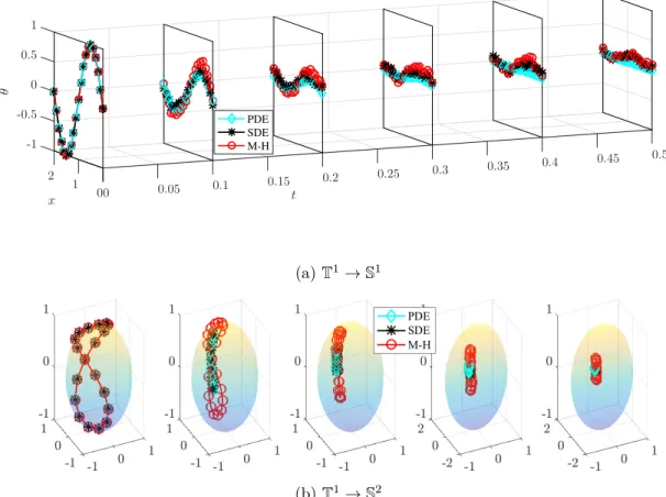
2.1 Dynamics of M-H algorithm (red circles), Langevin equation (black stars) and Landau-Lifshitz equation (cyan diamonds) at various instances of time. They follow each other to converge to equilibrium. In both panels: lattice lengthL= 2, space discretization
δx= N1 = 101 , time step size for M-H algorithmδt= N13 = 0.001, inverse temperature
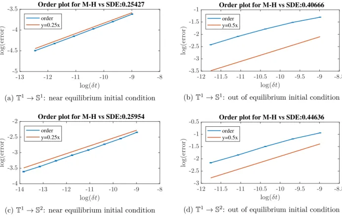
β =N3/2≈31.6, proposal sizeε=qN δtβ ≈0.0178. . . 49 2.2 Order of convergence for the error between M-H algorithm and Langevin equation
with respect to time step size δt= NJ β2ε2 forβ =N3/2. When the initial condition is near equilibrium, the order of convergence is approximately 0.25 as predicted in theorem 2.1.1. When the initial condition is out of equilibrium, the order is better than 0.25 and close to 0.5. In all four panels: lattice length L = 2, space discretization δx = N1 = 101 , time step size for M-H algorithm δt = N13, inverse temperatureβ =N3/2, proposal sizeε=qN δtβ . . . 50 2.3 Order of convergence for the error between M-H algorithm and Langevin equation
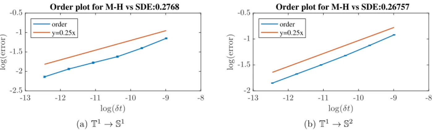
with respect to time step size δt = NJ β2ε2 for β = 1. The order of convergence is approximately 0.25 as predicted in theorem 2.1.1 with out of equilibrium initial condition. In both panels: lattice length L= 2, space discretization δx= N1 = 101, time step size for M-H algorithm δt= N13, inverse temperature β = 1, proposal size
ε=qN δtβ . . . 51 2.4 Order of convergence for the error between M-H algorithm and Landau-Lifshitz
equation with respect to lattice discretization size δx= N1. From Figure 2.1 the error between M-H algorithm and Langevin equation dominates over the error between Langevin equation and Landau-Lifshitz equation. The order of convergence is expected to be δt14 = δx since we choose δt =δx4 and it is approximately the case in 2.4a and 2.4b. The analytical results in thoerem 2.1.1 and 2.1.2 does not give as good convergence rate and demands worse scaling ofδt, β as function of N. The following parameters tested in numerical experiments are enough: Lattice lengthL= 2, initial space discretization δx = N1 = 101 , time step size for the M-H algorithmδt = N13, inverse temperature β= 1, proposal size ε=qN δtβ . . . 51
3.1 Order of convergence for the error between M-H algorithm and Langevin equation with respect to time step sizeδt= Nβε2. The order of convergence is close to 0.5. For the parameters: lattice length L= 1, number of spins N = 10, space discretization
δx= N1 = 101 , initial time step size for M-H algorithmδt= 10−3, inverse temperature
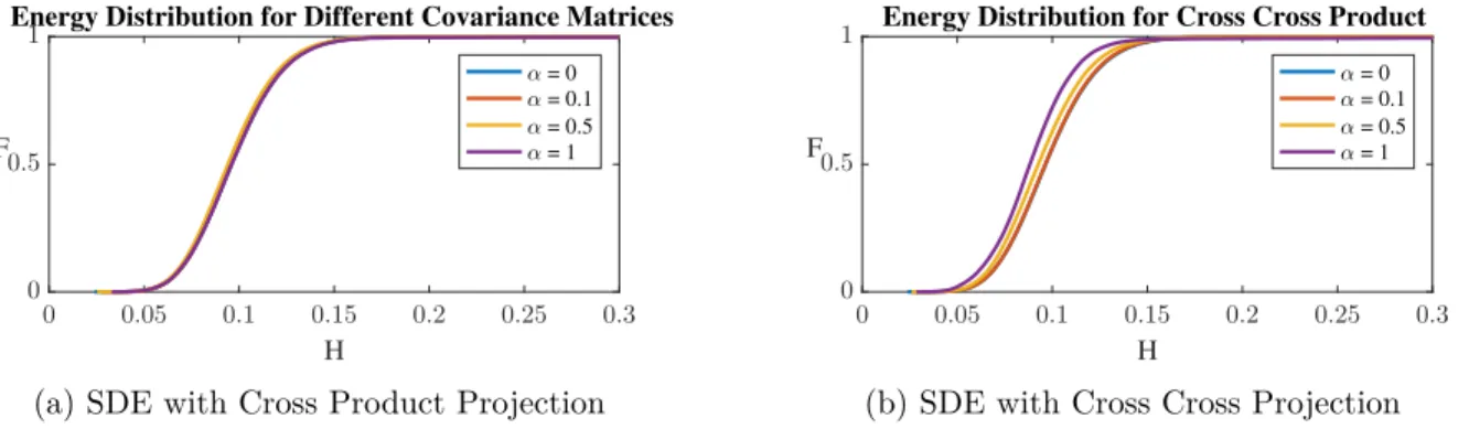
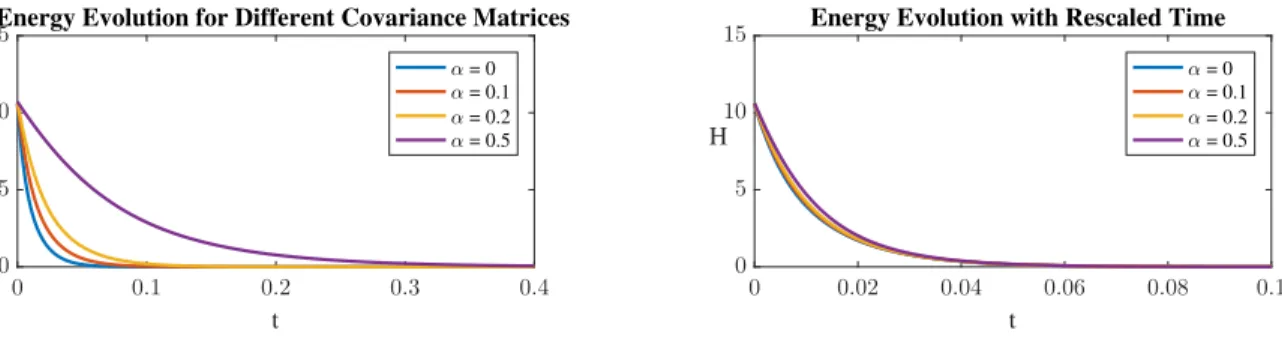
β = 1, proposal sizeε=qN δtβ , number of simulations E= 1000. . . 81 3.2 Distribution of energy H for colored noise SDE (1.6). α represents the decaying
3.3 Evolution of energyH for the PDE 3.61 withP being the cross product projection.
α represents the decaying rate of the eigenvalues for ¯CN, where thekth eigenvalue is
CHAPTER 1
Introduction
1.1 Overview
The Metropolis-Hastings (M-H) algorithm [1] is widely used in particle statistics for model estimations [2, 3, 4, 5, 6]. It constructs a discrete-time Markov chain to sample the desired probability distribution by accepting or rejecting proposed states. For applications in statistical physics, it is often the Gibbs or canonical distribution that is to be sampled. In this case, the algorithm accepts all the proposed new states with lower energy and often rejects the proposals with higher energy. Similar sampling can be achieved simulating a Langevin Stochastic differential equation (SDE) (1.3) that performs gradient descent with noise; it too has the Gibbs distribution as its steady-state distribution. This suggests that the Langevin SDE might be the optimal M-H algorithm in which all proposals are accepted.
For certain forms of probability distributions, the diffusion limit and therefore optimal scaling, of the random walk M-H algorithm has been obtained [7, 8, 9]. Specifically, for product measures in [7] and the Gibbs distribution of a lattice model in [8], the weak convergence to Langevin diffusions has been shown by comparing generator functions. For non-product form measures, the weak convergence to a stochastic partial differential equation was shown in [9]. These works consider the weak convergence only in equilibrium. Subsequent works [10, 11] consider scaling limits of out of equilibrium systems approaching equilibrium.
To address the question of trajectory-wise convergence, we study the XY and the classical Heisenberg lattice spin models [12] that play an important role in statistical physics to understand phase transitions and other phenomena including superconductivity [13, 14]. The XY and classical Heisenberg models are defined on a periodic d-dimensional lattice Td with δx = N1 the distance between adjacent vertices. Each spin sits at a lattice point and is described by a unit vector
model. The Hamiltonian of the system,
H =J X
<i,j>
kσi−σjk2, (1.1)
gives energy to misaligned neighboring spins where < i, j > represents nearest neighbors and
J = N2−d is a scaling factor. Denote σ as the total spin configuration of σi, i ∈ Td, the M-H algorithm accepts/rejects based on the Gibbs distribution defined as
ρ(σ) =Z−1exp(−βH(σ)), (1.2)
where β = (kBT)−1 is the inverse temperature and Z is the normalizing factor (aka partition function). The distribution is unaware of the confining geometry that the spins must remain in Sm. Rather, it is included in the proposal step of the M-H algorithm. Always accepting the proposal step leads to each spin behaving independently like Brownian motion on the surface of Sm.
Since the XY model and the classical Heisenberg model are widely used to study superconductors and ferromagnets, their critical properties are of interest. Asymptotic results on the total spin of the mean-field XY and classical Heisenberg models have been studied by large deviation theory and Stein’s method in [15, 16]. Numerically, Monte Carlo methods are used to verify analytical results about XY model in [6, 5] and classical Heisenberg model in [17, 18].
We will show the M-H algorithm applied to the above lattice system, in the limit of small perturbations in the proposal, produces equivalent trajectories to the overdamped Langevin equation,
dσi= P⊥σi(∆Nσi)dt+ P
⊥
σi
s
N βdWi
!
, (1.3)
(1.3) performs gradient descent on the energy defined by (1.1) with the added constraint that σi is confined to Sm, m = 1,2. In the case of S2 for the classical Heisenberg model, it is an SDE representation of the overdamped Landau-Lifshitz-Gilbert equation that has the Gibbs distribution as its invariant measure [19, 20].
Taking the number of lattice points,N, to infinity or equivalently the lattice spacingδx= N1 to zero, the limit of the deterministic part of (1.3) is the partial differential equation (PDE) called the harmonic map heat flow equation
∂tσ= P⊥σ(∆σ). (1.4)
In the S2 case, (1.4) is in the form of the overdamped Landau-Lifshitz equation [21]
∂tσ =−σ×(σ×∆σ). (1.5)
In [22] this Landau-Lifshitz equation was shown to be equivalent to the Harmonic map heat flow from Td→ S2. With the scaling J =N2−d, the Hamiltonian in (1.1) is the discrete form of the Dirichlet energy, R
Ω|∇σ|2dΩ, for this harmonic map heat flow. This suggests that by decreasing the temperature, the out of equilibrium dynamics of the M-H algorithm converge to the deterministic flow of (1.5) with large N for the classical Heisenberg model. We will show this equivalence by showing the convergence of the system of SDE (1.3) to the PDE (1.4) in the limit of large N with an appropriate scaling of the temperature to zero with N.
One method to obtain the deterministic limit of a stochastic system is to consider the hydro-dynamic limit with relative entropy bound [23, 24, 25]. Due to the geometric constraint in the XY and classical Heisenberg models, it is difficult to calculate the averages with respect to the Gibbs states as in [23, 24, 25] if the spin is expressed in Cartesian coordinates. One might try to use polar coordinates to do window averaging but the potential is not convex as in [25]. Since the hydrodynamic limit for the XY and the classical Heisenberg models are not fully understood, we choose an alternative approach of taking inverse temperature β to infinity along with particle number N → ∞.
method to our knowledge is to take the Taylor expansion of the M-H step and approximate it as a linear step. This truncation leads to a spin vector that does not stay on the sphere but the error for the subsequent steps is shown to converge in the limit asN → ∞with our system-size-dependent choice of parameters. Note that in the weak convergence result of M-H dynamics to diffusion processes [7, 8, 9], the assumption of equilibrium is essential to bound the error terms. The result in Chapter 2 only assumes that the M-H dynamics (and thus the SDE system) start from a deterministic initial condition satisfying a certain regularity condition. While the initial condition is assumed smooth, both the M-H and SDE dynamics immediately produce fluctuations, and the resulting trajectories are only close to the smooth deterministic PDE solution and not smooth themselves for all time. Therefore, standard energy bounding techniques cannot be used. To bound the error terms, we utilize scalings that are worse than those in the previously mentioned papers and are likely not optimal. We use numerical simulations to explore how tight these bounds appear to be. Taking N → ∞ in (1.3), the discrete Laplacian ∆N converges to the Laplacian operator ∆ and the collection of√N[dW1; dW2;· · ·; dWN] becomes time-space white noise and an SPDE limit can be obtained intuitively. There are two remaining gaps for this. First, the SDE is understood in Stratonovich form, the Itô understanding will introduce an extra Itô correction term −N
βσi in (1.3), which goes to infinity asN → ∞ for constantβ. Second, the discrete Laplacian ∆N makes (1.3) a finite difference approximation of the limiting SPDE. The convergence of finite difference approximation relies on the regularity of the limiting equation solution to have enough Taylor expansion terms. It is also known that the solution for the stochastic heat equation with white noise does not exist for dimension higher than one. White noise might not be smooth enough to get the convergence to an SPDE limit.
In Chapter 3, we therefore introduce spatially correlated noise to regularize the noise term restricting to theS2 case for simplicity. The Itô correction term of the limiting SDE (1.6) has the same size as the trace of the covariance matrix for the colored noise. Assuming the covariance matrix of the colored noise being trace class operator, the Itô correction term remains bounded in the limitN → ∞. We obtain a new Stratonovich SDE from the limiting M-H dynamics
dσ=−P CNPT∆Nσdt+
q
β−1N P C1/2
where σ = [σ1x;· · ·;σN x;σ1y;· · ·;σN y;σ1z;· · ·;σN z] is a 3N dimensional vector combining all 3-dimensional individual spin vectors,P is a 3N×3N matrix for projection onto the tangent plane of individual spins and CN is a 3N ×3N block diagonal covariance matrix. We will explain P and
CN in more detail in Chapter 3. With colored noise, the proposal density in M-H algorithm is not symmetric and the associated Metropolis dynamics are not sampling the Gibbs distribution (1.2) exactly. However, if P is chosen to be the cross product projection matrix, (1.2) can be shown to be the invariant measure of (1.6) from Fokker-Planck equation calculation in Section 3.2. The equation (1.3) with white noise is a special case of (1.6) when ¯CN is the identy matrix.
We propose a new nonlocal SPDE
(1.7)
∂
∂tσ(x, t) =P CP
T∆σ−β−1Tr(C)σ+qβ−1P ηC(x, t)
as the limit of (1.6), whereP can be either the cross product projection or the cross cross product projection, the operator
Cf(x) =
Z
Td
C(x−y)f(y)dy,
and ηC(x, t) is the noise white in time and colored in space. We conjecture that the deterministic part of (1.7) behaves like harmonic map heat flow equation (1.4) with rescaled time, and explore the drift part of (1.7) with numerical experiments.
1.2 Metropolis-Hastings algorithm
We include essential basic knowledge of M-H algorithm here as preparation for Chapter 2 and 3. Markov chain Monte Carlo (MCMC) methods are widely used in sampling complicated distribu-tions in statistics, computational physics, and computational biology. It constructs an aperiodic and positive recurrent Markov chain with the desired distribution as the unique invariant measure.
1.2.1 Acceptance-Rejection method
Though not an MCMC method, acceptance-rejection (A-R) sampling shares the key accept-reject step as in the M-H algorithm. Unlike the correlated samples in MCMC methods, the samples generated are independent in A-R method.
Assume the absolutely continous target density is
π(x) = 1
Kf(x),
wherex∈ RdandKis the unknown normalizing factor. The A-R method requires a distributionh(x) which can be sampled directly by some known methods and can bound f(x) by f(x)≤ch(x) ∀x. Then the following procedure is used to generate independent samples:
1. Generate a candidatex from h(x) and a uniform random variableu∈[0,1] 2. Ifu≤ chf((xx)), returnx as the result; otherwise repeat the process
In the first step, a ’wrong’ candidate is generated. The second step adjusts the probability of accepting this candidate and makes it proportional to π(·):
h(x) f(x)
ch(x) =
f(x)
c .
1.2.2 M-H algorithm
M-H algorithm samples the target distribution π(·) by constructing an ergodic Markov chain. The Markov process is determined by its transition probabilityp(x|y) and M-H algorithm finds a transition probability satisfying
(1.8)
π(x)p(y|x) =π(y)p(x|y).
The equation (1.8) is called the detailed balance and is a sufficient condition for π(·) to be the invariant measure of the corresponding Markov chain
Z
p(y|x)π(x)dx=
Z
p(x|y)π(y)dx=π(y).
the unique invariant measureπ(·). The ergodicity means that the time average of the process will converge to the ensemble average
lim T→∞
1
T
T
X
i=1
f(xi) =
Z
f(x)π(dx).
Thus the properties of the target distribution π(·) can be obtained from sampling the constructed Markov chain.
The idea similar to A-R method is used to find a transition probability satisfying detailed balance (1.8). A proposal densityp(x|y) that can be sampled directly generates the candidates and an accept/reject probability α(x|y) adjusts the transition probability to satisfy detailed balance (1.8)
(1.9)
π(x)p(y|x)α(y|x) =π(y)p(x|y)α(x|y).
If 0< π(x)p(y|x)< π(y)p(x|y), then the probability from x→y is smaller than fromy →x, to compensate α(x|y) can be made smaller
α(x|y) = π(x)p(y|x)
π(y)p(x|y), α(y|x) = 1
so that detailed balance still holds. It is similar forπ(x)p(y|x)> π(y)p(x|y)>0. The accept/reject rate is defined as
α(x|y) =
minππ((xy))pp((xy||xy)),1 ifπ(y)p(x|y)>0
1 otherwise
(1.10)
If the proposal densityp(x|y) is chosen to be symmetric
p(x|y) =p(y|x),
the accept/reject rate can be simplified as
α(x|y) = min
π(x)
π(y),1
.
The M-H algorithm samples the target distribution with the following procedure: 1. At timestepn, generate candidate ˜xn+1 from p(·|xn)
2. Calculate accept rateα(˜xn+1|xn)
3. Generate uniform random numberu∈[0,1] 4.
xn+1 =
˜
xn+1 if u≤α(˜xn+1|xn)
xn else 5. Repeat the procedure for timestep n+ 1
One choice of proposal is p(y|x) = q(y−x) and this is the random walk M-H algorithm. A random variablez is generated from q(z) and the candidate is given byy=x+z.
1.2.3 Convergence of random walk M-H algorithm
In random walk M-H algorithm, if the size of the proposalzin q(z) is small, the generate process will stay in a small neighborhood for a long time. If the size of the proposal is too large, it is always rejected and the generate process stays at isolated values. An appropriate size of the proposal has to be chosen to better explore the target space.
The optimal scaling problem has been studied by [7, 26, 8, 9] for weak convergence of M-H algorithm in equilibrium. For certain forms of distributions, in the high dimensional limit random walk M-H algorithm behaves like a diffusion process and optimal scaling can be obtained accordingly. There are also subsequent works [10, 11] considering scaling limits of out of equilibrium systems approaching equilibrium.
The early works have been summarized in [27]. For target measure
π(x) =Y i
f(xi) (1.11)
dimensional, and the accept rate
a=
¨
π(x)p(y|x)α(y|x)dydx= lim n→∞n
−1(number of accepted proposals) (1.12)
is close to 0.234. For the Metropolis adjusted Langevin algorithms (MALA) applied to target measure in product form [26], the clever use of gradient of target distribution in proposal distribution leads to a larger optimal variance ofO(d−13), and a larger optimal asymptotic acceptance rate 0.574. The idea is to prove the generator for the M-H algorithm converges to the generator of the limiting diffusion process.
The work in [9] analyzes the nonproduct target distribution with Radon-Nikodym derivative
dπ(x)
dπ0(x)
=Mexp(−ψ(x)), (1.13)
CHAPTER 2
M-H Dynamics with White Noise 1
The Hamiltonian (1.1) of the lattice spin models is a discrete form of a version of a Dirichlet energy, signifying a relationship to the Harmonic map heat flow equation. The Gibbs distribution (1.2), defined with the Hamiltonian (1.1), is used in the M-H algorithm to generate dynamics tending towards an equilibrium state. In the limiting situation when the inverse temperature is large, we establish the relationship between the discrete M-H dynamics and the continuous Harmonic map heat flow associated with the Hamiltonian. We show the convergence of the M-H dynamics to the Harmonic map heat flow equation in two steps: First, with fixed lattice size and proper choice of proposal size in one M-H step, the M-H dynamics acts as gradient descent and will be shown to converge to a system of Langevin stochastic differential equations (SDE). Second, with proper scaling of the inverse temperature in the Gibbs distribution and taking the lattice size to infinity, it will be shown that this SDE system converges to the deterministic Harmonic map heat flow equation.
In Section 2.1 we present the main results in two parts. First, we state the convergence of M-H dynamics to the SDE system (1.3) as the proposal size of M-H step goes to zero, then we state the convergence of the SDE system (1.3) to the deterministic PDE (1.4) as the lattice size goes to infinity and temperature to zero. The key steps of the proofs are given in Sections 2.2 and 2.4 for the more complicated classical Heisenberg model from T1→S2. The proof for the XY model follows similarly and we omit it. For the M-H to SDE (1.3) proof in Section 2.2, we apply a similar approach as in [9], by first Taylor expanding the M-H step, keeping only the first three terms, then computing the required conditional expectations with respect to the Gaussian random variables to
1
obtain the drift and diffusion terms of an Euler step for the diffusion process. Then, the difference between the M-H and SDE dynamics inL2 norm is bounded by a Grönwall inequality. The details on the error bounds are given in Section 2.3. For the SDE (1.3) to PDE (1.4) proof in Section 2.4, we compare the SDE system with the finite difference approximation of the harmonic map heat flow equation (1.4). The difference between the SDE and ODE system is governed by another diffusion process. We will rescale this process and show the rescaled error is bounded for a long time using stopping time. These convergence results are supported by numerical simulations of the systems in Section 2.5.
2.1 Main results
In this section we will explain how we apply M-H algorithm to the XY and classical Heisenberg models, and state our main results. Our first result is that the M-H dynamics is close to a stochastic Euler scheme for the SDE (1.3) in Itô understanding. The bound on the error between the M-H dynamics and the SDE (1.3) is accomplished using arguments similar to the convergence of the stochastic Euler method. Our second result bounds the error between the SDE system and the finite difference approximation of the harmonic map heat flow equation (1.4).
2.1.1 Metropolis-Hastings step
Here, we explicitly state the M-H dynamics for XY and classical Heisenberg models we consider with Hamiltonian given by (1.1) for the case d= 1.
Consider a set of spins evolving in time, σin for particle i= 1. . . N and time stepn≥0 with time step size δt. To create the proposal, take the normal random vector
wni =
z1
z2
, withz1, z2∼ N(0,1)
for the XY model and three-dimensional normal random vector
wni =
z1
z2
z3
, withz1, z2, z3 ∼ N(0,1),
vectorνin=Pσ⊥n i(w
n
i) =wni −(win, σin)σin. Since we are trying to get a trajectory-wise convergence result, it is convient to imbed the M-H algorithm and the SDE dynamics in the same probability space. To this end, we define
win≡ Wi((n+ 1)√δt)−Wi(nδt)
δt ,
where Wi,1≤i≤N are the Brownian motion in (1.3). At time stepn the proposal for next time step is
˜
σni = expσn i(εν
n
i), 1≤i≤N, (2.1)
with expσn
i the exponential map and εthe proposal size. The values σ
nand ˜σn are used to denote the total spin configurationσin,1≤i≤N at time step nand the total proposal spin configuration ˜
σin,1≤i≤N. The proposal ˜σn is accepted with probability
α= 1∧e−βδH, (2.2)
and rejected otherwise, where
δH =H(˜σn)−H(σn) = N
X
j=1
∂H ∂σn
j
·(˜σjn−σnj) + 2J
N
X
j=1
(˜σnj −σjn)·(˜σjn−σjn)
−J
N
X
j=1
(˜σnj −σjn)·(˜σjn+1−σjn+1+ ˜σjn−1−σnj−1)
(2.3)
is the difference between the Hamiltonian (1.1) of the proposal ˜σnand of the current spin configuration
σn. Then
σn+1 =κnσ˜n+ (1−κn)σn, κn∼Bernoulli(α(˜σn, σn)).
Repeating this step, we create a discrete Markov process at time steps n+ 1, n+ 2, . . .and we will show the convergence of the Markov chain to the solution to the Langevin SDE system (1.3).
classical Heisenberg model
P⊥σn i(w
n i) =
σin×wni
−σn
i ×(σin×win) =win−σin(σin)Twni as both lead to random walk on the sphere (see Appendix A).
2.1.2 Convergence of Metropolis dynamics to SDE system
First we are going to show the convergence from M-H dynamics to Langevin SDEs with fixed number of particlesN as the proposal sizeε→0. Intuitively, using the Taylor series truncation of the proposal, the approximation of one M-H step leads to an expression that looks like one Euler step for simulating the SDE (1.3) in Itô sense.
Let Ftdenote the filtration generated by the Brownian motionWi in (1.3) and Bernoulli random variablesκn atnδt, we denote the conditional expectation E[·|Fnδt] by En[·].
The drift over one step of the Metropolis-Hastings algorithm for the i-th particle for smallεis approximated by
En
h
σni+1−σnii≈ −1 2βε
2P⊥
σn i
∂H ∂σn
i
!
−ε2σin, (2.4)
where P⊥σn
i =I−σ n
i(σin)T is the projection onto the tangent plane of σin. Denoting the noise contribution over one step as
Γni ≡σni+1−σin−En
h
σin+1−σnii, (2.5)
it is approximated by
Γni ≈ενin=εP⊥σn i(w
n
i). (2.6)
Thus, one step of the Metropolis-Hastings algorithm is approximately given by
σni+1−σin≈ −1 2βε
2P⊥
σni
∂H ∂σin
!
−ε2σni + P⊥σn i(εw
n
Definingβε2 =N δtwhereδt is the time step size, the above equation changes to
σin+1 ≈σni −1 2NP
⊥
σn i
∂H ∂σni
!
δt−N
β σ
n iδt+ P
⊥
σn i
s
N βw
n i
√
δt
!
. (2.8)
Since ∂σ∂Hn i
= 2J(2σni −σin+1 −σni−1) and J = N when d= 1, the above is the Euler step for the Langevin SDE (1.3) in Itô interpretation
dσi= P⊥σi(∆Nσi) dt−
N
β σidt+ P ⊥
σi
s
N βdWi
!
. (2.9)
This intuitive idea leads to the first result:
Theorem 2.1.1. Define the piecewise constant interpolation of M-H dynamics asσ¯i(t),
¯
σi(t) =σin nδt≤t <(n+ 1)δt, (2.10)
and σi(t) as the solution for the Langevin SDE system (2.9)with initial condition kσi(0)k= 1,1≤
i≤N. If we think of the proposal in M-H step coming from the noise
εwni =
q
N β−1[W
i((n+ 1)δt)−Wi(nδt)],
then we have the following strong convergence result:
E
"
sup 0≤s≤t
kσi(s)−¯σi(s)k2
#
≤C1 √
δtexp(C2T), t∈[0, T],1≤i≤N, (2.11)
for any T ∈(0,∞), where C1, C2 are functions of N, β, J, T and independent of the choice ofi and
δt.
Remark 2.1.2. The equation(2.9)is equivalent to the SDE in Stratonovich sense (1.3)which gives dkσik2= 2σi·dσi = 0 to make σi stay on the unit sphere.
Remark 2.1.3. Theorem 2.1.1 is a trajectory-wise convergence result.
2.1.3 Convergence of SDE system to the Landau-Lifshitz equation
Theorem 2.1.2. For the harmonic map heat flow equation (1.4) with periodic boundary condition and initial condition satisfing
kσ(·,0)k= 1,k∇σ(·,0)k≤λ, (2.12)
for some λ as in [22], the solution exists and is smooth. Denote the finite difference approximation
of (1.4)as
d˜σi =P⊥σ˜i(∆Nσ˜i), k˜σik= 1 (2.13)
and k˜σi(t)−σ(iδx, t)k→0 on any fixed time interval where the solution remains well defined, when the space discretizationδx= N1 goes to zero [28, Theorem 1].
For any 0< p < 12, there exist a constant γ >1, β=Nγ and constants C1, C2 independent of
N, such that if
N
β
1−p
T +C1 1
N
N
β
1−2p!
eC2T ≤1,
then the difference between the SDE (2.9) and the finite difference approximation (2.13) has the following bound
E
"
sup 0≤s≤t
1
N
N
X
i=1
kσi(s)−σ˜i(s)k2
#
≤
N
β
p/2
, t∈[0, T]. (2.14)
As γ > 1,Nβ is small when N is large, so the difference between the SDE system and finite difference approximation of the PDE is bounded by a small term for a long time T that goes to ∞ with N → ∞. The solution for PDE is smooth so the finite difference approximation is close to the PDE solution as shown in [28].
Remark 2.1.4. The choice of γ depends on p with the following relation
N
β
p/2
N3 ≤1.
For a uniform bound in 0≤t≤T, we needp < 12 soγ >13. For a bound with some fixedt∈[0, T], we only need p <1 and γ >7. We do not believe this bound is sharp for the convergence result at all, which will be addressed in Section 2.5 when we perform numerical simulations of these models.
2.2 Metropolis-Hastings dynamics to SDE system
In this section the convergence of the M-H algorithm to the SDE (2.9) for the classical Heisenberg model will be shown by calculating the drift and diffusion of one M-H step, which is approximately a stochastic Euler step for (2.9). Then the error estimation of stochastic Euler’s method is used to give a bound on the difference between M-H and SDE dynamics with proposal sizeε→0. Here the basic steps are outlined, the detail of error estimation is given in Section 2.3.
Remark 2.2.1. The proof for the XY model will be similar, one only needs to change the random
vector νin on the tangent plane as a two-dimensional vector.
2.2.1 Set-up
In the calculation to follow, we have the following assumptions and notations.
The number of the particles N on unit length is fixed and the limiting caseε→0 is considered. We have β, J as functions ofN so they are also regarded as constant.
In the calculation, the proposal ˜σni is approximated by normalizingσni +ενin
˜
σni = expσn i(εν
n i)≈
σni +ενin
kσni +ενink.
By Taylor expanding σ n i+εν
n i
kσn i+εν
n ik
, the proposal ˜σni can be approximated by orderε andε2 expansion
˜
σin≈σin+ενin,
˜
σin≈σin+ενin−1 2ε
2(νn
i ·νin)σin.
(2.15)
The proof of the following Lemma is shown in Section 2.3.
Lemma 2.2.1. Denote
ani ≡˜σni − σ n i +ενin kσin+ενink,
cni ≡˜σni −(σni +ενin), dni ≡˜σni −
σin+ενin−1 2ε
2(νn
i ·νin)σin
.
Then Ehkanikki≤A kε3k,E
h
kcnikki≤C
kε2k and E
h
Using the approximation (2.15), δH in (2.3) can be written as
δH =ε∂H ∂σin ·ν
n
i +Rni +hni ≈O(ε),
Rni ≡εX
j6=i
∂H ∂σn
j
·νjn≈O(ε),
hni ≡X j
∂H ∂σnj ·c
n j + 2J
X
j
δσjn·δσjn−JX
j
δσjn·(δσnj+1+δσnj−1)≈O(ε2),
(2.16)
and we only keep theεterm in δH in the following calculation soδH is approximated by a normal random variable. We are going to show the calculation for one specific particlei so we takei-th term ∂σ∂Hn
i
·νin and the summation of j6=iterms as a single termRni.
2.2.2 Drift
Proposition 2.2.1. Let{σn}be the Markov chain given by the Metropolis-Hastings algorithm, and
{σni} the spin fori-th particle at time stepn. Then
En
h
σni+1−σini=−1 2βε
2P⊥
σn i
∂H ∂σin
!
−ε2σni +θin, (2.17)
where the error term
θin≡En
h
σin+1−σini− −1 2βε
2P⊥
σn i
∂H ∂σni
!
−ε2σni
!
(2.18)
satisfies E
kθink2
≤Cε6.
In the calculation we keep the order ε2 term. The remainder is order ε3 and will be shown to be bounded in the error estimation for M-H and SDE dynamics. The basic steps are given in the following calcuation, for details of the error estimation see Section 2.3.
Since σin+1= expσn i(εν
n
i) with probability 1∧e−βδH and stay σin otherwise,
(2.19) En
h
σin+1−σini=En
h
expσn i(εν
n
i)−σni 1∧e
−βδHi
≈En
"
ενin−ε 2 2(ν
n
i ·νin)σin+dni
!
1∧e−βδH
#
=εEn
h
νin1∧e−βδHi−ε 2 2En
h
(νin·νin)σni 1∧e−βδHi
+En
h
We drop the third term in the last line of (2.19) as it is an ε3 term:
E
h d
n i
1∧e−βδH i
≤E[kdnik]≤Cε3,
since 0<|1∧e−βδH|<1.
For the second term in the last line of (2.19), since 1∧e−βδH ≈1 +O(ε) we have that
ε2
2En
h
(νin·νin)σin1∧e−βδHi=En
"
ε2
2(ν n
i ·νin)σin
#
+O(ε3) =ε2σin+O(ε3).
This corresponds to the Itô correction for (1.3).
The first term in the last line of (2.19) is the most difficult one to approximate. Using the notation in (2.16)
1∧e−βδH = 1∧e−β
ε∂σn∂H i
·νin+Rni+hni
≈1∧e−β
ε∂σn∂H i
·νin+Rni
+O(ε2),
sincehni ≈O(ε2), to write it as
En
h
ενin1∧e−βδHi=En
"
ενin 1∧e−β
ε∂σn∂H i
·νn i+Rni
!#
+O(ε3).
For any orthonormal basis {b1, b2, b3} inR3, the normal random vector win can be expressed as
win= (win·b1)b1+ (win·b2)b2+ (wni ·b3)b3
and (wni ·b1),(win·b2),(win·b3) are independent standard normal random variables. Denote
r1 = (win·b1), r2 = (win·b2), r3 = (wni ·b3),win=r1b1+r2b2+r3b3. Chooseb1, b2 two orthonormal vectors on the tangent plane ofσin and b3=σni,
νin= Pσn i(w
n
where r1, r2 ∼ N(0,1) are independent. Then,
En
"
ενin 1∧e−β
ε∂σn∂H i
·νn i+Rni
!#
=En
"
εr1b1 1∧e
−β
εr1∂σn∂H i
·b1+εr2∂σn∂H i
·b2+Rn i
!#
+En
"
εr2b2 1∧e
−β
εr1∂σn∂H i
·b1+εr2∂σn∂H i
·b2+Rn i
!#
.
(2.20)
The two terms on the right are similar in form so we only show the calculation for the first one and the second one follows similarly.
Remark 2.2.2. For the XY model, the projection of the normal random vector onto the tangent
plane of σin is represented by the formr1b1, where r1 ∼N(0,1). The other parts of the calculation
basically stays the same.
Using tower property of conditional expectation for the first term on the RHS of (2.20), we have
En
"
εr1b1 1∧e
−β
εr1∂σn∂H i
·b1+εr2∂σn∂H i
·b2+Rni
!#
=En
(
En
"
εr1b1 1∧e
−β
εr1∂σn∂H i
·b1+εr2∂σn∂H i
·b2+Rn i
! r2, R
n i
#)
.
We recall the following Lemma 2.4 in [9]. (See also [7].)
Lemma 2.2.2. For z∼ N(0,1),
E
h
z1∧eaz+bi=aea
2 2+bΦ
− b |a|− |a|
, (2.21)
for any real constants a, b, andΦ(·) is the CDF for the standard normal random variable.
The proof of this Lemma is the direct result of the integration for the expectation. And the Lemma gives
(2.22) En
"
εr1b1 1∧e
−β
εr1∂σn∂H i
·b1+εr2∂σn∂H i
·b2+Rn i
! r2, R
n i
#
=−βε2 ∂H ∂σin ·b1
!
b1e
βε ∂H ∂σn i
·b1
2 2 −βεr2
∂H ∂σn i
·b2−βRni Φ
εr2∂σ∂Hn i
·b2+Rni
ε ∂H ∂σn i
·b1
− βε∂H ∂σin ·b1
Before taking the expectation over r2, we further simplify this expression by noting that eO(ε)= 1 +O(ε) resulting in
En
"
εr1b1 1∧e
−β
εr1∂σn∂H i
·b1+εr2∂σn∂H i
·b2+Rni
! r2, R
n i
#
≈ −βε2 ∂H ∂σn
i ·b1
!
b1+O(ε3)
!
Φ
εr2∂σ∂Hn i
·b2+Rni
ε ∂H ∂σn i
·b1
+O(ε)
.
(2.23)
For a mean zero Gaussian random variablez, we know
E[Φ(z)] =E
Φ(z)−1 2+ 1 2 = Z ∞ −∞
Φ(z)−1 2 +
1 2
p(z)dz= 1 2,
as Φ(z)−1
2 is an odd function and the probability density function p(z) is even. Notice thatRni =εP
j6=i∂σ∂Hn j
·νjn is a sum of independent mean zero Gaussian random variables, soεr2∂σ∂Hn
i
·b2+Rni is a Gaussian random variable with mean 0, therefore
En
−βε2
∂H ∂σni ·b1
!
b1Φ
εr2∂σ∂Hn
i ·b2+R n i ε ∂H ∂σn i
·b1
=− 1 2βε 2 ∂H
∂σin ·b1
!
b1.
The second term on the RHS of (2.20) follows similarly,
En
"
εr2b2 1∧e
−β
εr1∂σn∂H i
·b1+εr2∂σn∂H i
·b2+Rni !# =−1
2βε 2 ∂H
∂σin ·b2
!
b2+O(ε3).
Combining the above
En
h
σni+1−σnii≈ −1 2βε
2P⊥
σn i
∂H ∂σin
!
−ε2σin,
where ∂σ∂Hn i
= NJ2∆Nσin and ∆Nσni =N2(σin+1+σni−1−2σni) denotes the discrete Laplacian.
2.2.3 Diffusion
Recall Γni in (2.5),
Γni =
ενin+cni −Enhσin+1−σnii with probabilityα
−En
h
with accept rate α in (2.2). Since Enhσin+1−σniiis an order ε2 term andα≈1 with smallε, we are going to show
Γni ≈ενin.
Proposition 2.2.2. The diffusion term
Γni =σni+1−σin−Enhσin+1−σini=ενin+φni, (2.24)
where
φin≡Γni −ενin=σin+1−σin−Enhσin+1−σini−νin (2.25)
is a random variable with meanE[φni] = 0, varianceE
kφnik2
≤Cε3, and covarianceE[φni ·φmi ] = 0
for n6=m.
Proof. For the mean
φni =σin+1−σin−En
h
σni+1−σini−ενin,
thenE[φni] =E
h
σni+1−σin−En
h
σni+1−σini−ενini= 0. For the variance,
E
h
kφnik2i=E
expσni(εν
n
i)−σin−En
h
σni+1−σini−ενin
2
1∧e−βδH
+E −εν n i −En
h
σni+1−σini
2
1−1∧e−βδH
=E c n i −En
h
σni+1−σini
2
1∧e−βδH
+E −εν n i −En
h
σni+1−σini
2
1−1∧e−βδH
.
(2.26)
The first term in the last line of (2.26)
E
c
n i −En
h
σin+1−σnii
2
1∧e−βδH
≤E c n i −En
h
σin+1−σnii
412
E
1∧e−βδH2
12
C
E
h
kcnik4i+E
En
h
σni+1−σini
412
≤Cε4,
asEnhσni+1−σini=−1 2βε
2P⊥
σn i ∂H ∂σn i
−ε2σni +O(ε3) and E
kcnik4
For the second term in the last line of (2.26), since 1−
1∧e−βδH =
e
0−e0∧(−βδH)
≤ |βδH|,
we observe
E
−εν
n i −En
h
σin+1−σini
2
1−1∧e−βδH
≤E
−εν
n i −En
h
σni+1−σini
412
E
h
|βδH|2i 1 2
≤Cε3,
for some constantC, since−ενn i −En
h
σni+1−σn i
i
=−ενn
i +O(ε2) and δH =ε
P
j ∂σ∂Hn j ·ν
n
j +O(ε2) are both order εterm.
Combining the above, the variance in (2.26) is bounded byEk
φnik2≤
Cε3.
For the covariance ofφni, φmi at different time stepsn > m, andζ =x, y, zdenotes the coordinates of the vector,
E
h
φni,ζφmi,ζi=E
h
En
h
φni,ζφmi,ζii=E
h
φmi,ζEn
h
φni,ζii=E
h
φmi,ζ0i= 0.
Remark 2.2.3. In fact, the error term isE
kφnik2
∼O(ε3) and this determines the order of the convergence in Theorem 2.1.1. The detail of calculation is given in Section 2.3.3.
2.2.4 Error estimation
For the error estimation, we apply similar techniques as in the proof of stochastic Euler’s method. Take σi,¯σi as in Theorem 2.1.1. For simplicity we denoteµi(σ) = P⊥σi(∆Nσi)−
N
βσi, ψi(σ) = √
N β(I−σiσiT) the coefficients in (2.9). When N, J, β are fixed andkσik= 1, the coefficient µ, ψ are Lipschitz continuous in each coordinates of x. From Theorem 5.2.1 in [29], the SDE system has a unique solution.
Now we have the following estimate on the error.
Proposition 2.2.3. Define the error e(t) between M-H interpolation σ¯i and SDE (2.9) solution σi as
e(t)≡ sup 1≤i≤N,0≤s≤tE
h
kσi(s)−σ¯i(s)k2
i
. (2.27)
For any fixed T >0,e(t) is bounded by
e(t)≤C(N, J, β, T) √
Proof. For the proof we are going to showe(t) satisfies the Grönwall inequality (Ci denotes some constant bound):
e(t)≤(C1T+C2)
Z t
0
e(s)ds+C3 √
δt+C4δt+C5δt2
, (2.29)
soe(t)≤C3 √
δt+C4δt+C5δt2
exp (C1T(T +C2)). Since ¯σi(t) = σ
bt δtc
i = σ0i +
Pb
s δtc−1 j=0
σji+1−σij and both σi,σ¯i start from the same initial condition, from definition ofe(t) and θni in (2.18), Γni in (2.5), φni in (2.25):
e(t) = sup 1≤i≤N,0≤s≤tE
h
kσi(s)−¯σi(s)k2
i
= sup
1≤i≤N,0≤s≤tE
Z s 0
µi(σ(u))du+
Z s
0
ψi(σ(u))dWi(u)− bs
δtc−1
X
j=0
En
h
σij+1−σjii+ Γji
2 = sup
1≤i≤N,0≤s≤t E " Z s 0
µi(σ(u))du+
Z s
0
ψi(σ(u))dWi(u)− bs
δtc−1
X
j=0
µi(σj)δt+ενij +θ j i +φ
j i 2#
where µi(σj)δt=Rjδt(j+1)δtµi(¯σ(u))du and ενij =
R(j+1)δt
jδt ψi(¯σ(u))dWi. Applying Hölder’s inequality and E|X+Y|2≤2EX2+Y2produces
(2.30)
e(t)≤C sup 1≤i≤N,0≤s≤tE
Z bs
δtcδt 0
µi(σ(u))−µi(¯σ(u))du
2 +
Z bs
δtcδt 0
ψi(σ(u))−ψi(¯σ(u))
dWi
2 + Z s bs δtcδt
µi(σ(s))ds
2 + Z s bs δtcδt
ψi(σi(s))dWi
2 + bs δtc−1
X
j=0
θji
2 + bs δtc−1
X
j=0
φji
2 .
Using Hölder inequality for the first term in (2.30) with the coordinate ζ =x, y, z
Z bs
δtcδt 0
µi,ζ(σ(u))−µi,ζ(¯σ(u))du
2 ≤
Z bs
δtcδt 0
µi,ζ(σ(u))−µi,ζ(¯σ(u))
2
du
Z bs
δtcδt 0
sinceµi is Lipschitz,
Z bδtscδt
0
µi,ζ(σ(u))−µi,ζ(¯σ(u))
2
du≤C1
Z bδtscδt
0
(σi,ζ(u)−σ¯i,ζ(u))2du,
combineζ =x, y, z terms,
sup 1≤i≤N,0≤s≤tE
Z bs
δtcδt 0
µi(σ(u))−µi(¯σ(u))du
2 ≤C1t
Z t
0
e(s)ds.
Applying Itô isometry to the second term of (2.30) for the x coordinate
E
Z bs
δtcδt 0
ψi(σ(u))−ψi(¯σ(u))dWi(u)
!2
x
=E
Z bs
δtcδt 0
¯
σxi(¯σxidWix+ ¯σiydWiy+ ¯σizdWiz)−σix(σxidWix+σiydWiy+σzidWiz)
!2
=E
" Z bs
δtcδt 0
(¯σix)2−(σxi)2dWix
!2
+
Z bs
δtcδt 0
¯
σxiσ¯iy−σxiσyidWiy
!2
+
Z bs
δtcδt 0
¯
σxiσ¯iz−σxiσizdWiz
!2#
=E
" Z bs
δtcδt 0
(¯σxi)2−(σix)22du+
Z bs
δtcδt 0
(¯σixσ¯iy−σixσiy)2du+
Z bs
δtcδt 0
(¯σxiσ¯iz−σizσzi)2du
#
.
Since
(¯σxi)2−(σix)22 ≤(|¯σix|+|σix|)2(¯σix−σix)2 ≤4(¯σxi −σxi)2,
(¯σxiσ¯yi −σixσyi)2 = ((¯σix−σix)¯σiy+σxi(¯σyi −σiy))2 ≤2(¯σxi −σxi)2(¯σiy)2+ 2(σxi)2(¯σiy−σyi)2,
(¯σxiσ¯zi −σxiσiz)2= ((¯σxi −σix)¯σzi +σxi(¯σzi −σiz))2 ≤2(¯σix−σix)2(¯σzi)2+ 2(σxi)2(¯σzi −σzi)2,
then
(2.31) E
Z bs
δtcδt 0
ψi(σ(u))−ψi(¯σ(u))dWi(u)
!2
x
≤CE
" Z bs
δtcδt 0
(¯σxi −σix)2+ (¯σiy−σiy)2+ (¯σzi −σzi)2ds
#
second term in (2.30) is bounded by
sup 1≤i≤N,0≤s≤tE
Z bs
δtcδt 0
ψi(σ(u))−ψi(¯σ(u))
dWi
2 ≤C2
Z t
0
e(s)ds.
For the third term in (2.30)
Z s bs δtcδt
µi(σ(s))ds
2
≤C3δt2,
sincekσik= 1 and s−δtsδt≤δt.
Apply Itô isometry again for the fourth term in (2.30),
E Z s bs δtcδt
ψi(σi(s))dWi
2
≤C4δt.
From Cauchy inequality and E
θ j i 2
≤Cε6 in Proposition 2.2.1, the fifth term in (2.30) is bounded by E bs δtc−1
X
j=0
θij
2 ≤ s δt b s δtc−1
X j=0 E θ j i 2
≤C5
t
δt
2
ε6 =C6δt.
From Proposition 2.2.2,Ehφji ·φkii≤Cδjkε3 with δjk the Kronecker delta, the sixth term in (2.30)
E bs δtc−1
X
j=0
φji
2 = bs δtc−1
X j=0 E φ j i 2
≤C7
t
δt
ε3 ≤C8 √
δt.
Combining all above, we get the Grönwall inequality (2.29).
Remark 2.2.4. In Grönwall inequality, the C3 √
δtterm decides the order of convergence. It comes
from E " Pb s δtc−1 j=0 φ
j i 2#
, which we show as O(ε3) term in 2.3.3.