Asymptotics for High Dimension, Low Sample Size data
and Analysis of Data on Manifolds
Sungkyu Jung
A dissertation submitted to the faculty of the University of North Carolina at Chapel Hill in partial fulfillment of the requirements for the degree of Doctor of Philosophy in the Department of Statistics and Operations Research (Statistics).
Chapel Hill 2011
Approved by:
Advisor: : Dr. J. S. Marron
Reader: : Dr. Mark Foskey
Reader: : Dr. Jason Fine
Reader: : Dr. Yufeng Liu
c
ABSTRACT
SUNGKYU JUNG: Asymptotics for High Dimension, Low Sample Size data and Analysis of Data on Manifolds.
(Under the direction of Dr. J. S. Marron.)
The dissertation consists of two research topics regarding modern non-standard data
an-alytic situations. In particular, data under the High Dimension, Low Sample Size (HDLSS)
situation and data lying on manifolds are analyzed. These situations are related to the
sta-tistical image and shape analysis.
The first topic is an asymptotic study of the high dimensional covariance matrix. In
partic-ular, the behavior of eigenvalues and eigenvectors of the covariance matrix is analyzed, which
is closely related to the method of Principal Component Analysis (PCA). The asymptotic
behavior of the Principal Component (PC) directions, when the dimension tends to infinity
with the sample size fixed, is investigated. We have found mathematical conditions which
characterize the consistency and the strong inconsistency of the empirical PC direction
vec-tors. Moreover, the conditions where the empirical PC direction vectors are neither consistent
nor strongly inconsistent are revealed, and the limiting distributions of the angle formed by
the empirical PC direction and the population counterpart are presented. These findings help
to understand the use of PCA in the HDLSS context, which is justified when the conditions
for the consistency occur.
The second part of the dissertation studies data analysis methods for data lying in curved
manifolds that are the features from shapes or images. A common goal in statistical shape
analysis is to understand variation of shapes. As a means of dimension reduction and
visual-ization, there is a need to develop PCA-like methods for manifold data. We propose flexible
extensions of PCA to manifold data: Principal Arc Analysis and Analysis of Principal Nested
Spheres. The methods are implemented to two important types of manifolds. The sample
space of the medial representation of shapes, frequently used in image analysis to
parame-terize the shape of human organs, naturally forms curved manifolds, which we characparame-terize
shape space, proposed by Kendall. The proposed methods in the dissertation capture major
variations along non-geodesic paths. The benefits of the methods are illustrated by several
ACKNOWLEDGEMENTS
I thank Professor Steve Marron for his advice and support. His support enabled me to enjoy my
research and to complete the dissertation work successfully. He helped me explore the subject
with his keen insight, and provided many opportunities for various kinds of collaborative
research. Every result in the dissertation is indepted to his guidance.
This dissertation work would have not been completed without valuable comments and
suggestions of coauthors. Professor Arush Sen lead me to take another leap in the theoretical
part of the dissertation in Chapter 3. Dr. Mark Foskey proposed to use small circles, and
investigations since then results in the work presented in Chapter 6. Professor Ian Dryden
introduced statistical shape analysis in which Chapter 7 is rooted. Professor Steve Pizer
intro-duced the broad area of image analysis and motivated to develop Part II of the dissertation.
I wish to express my sincere appreciation to senior researchers for their valuable advice.
Professor Steve Pizer has been a great mentor. Conversations with him on topics ranging from
personal life decisions to deep mathematical questions have helped me a lot during the Ph.D.
program. Professor Jason Fine and Professor Yufeng Liu gave me advices in making difficult
decisions. I also appreciate valuable academic discussions and conversations with Professor
Stephan Huckemann, Professor Anuj Srivastava, Professor Hongtu Zhu, Dr. Xiaoxiao Liu,
Dr. Ja-Yeon Jeong and the community of MIDAG.
My life at Chapel Hill during the program was happy and fulfilling. I can not imagin it
without friends: Classmates, gangs who flocked at Baity Hill and Finley Forest, and basketball
and tennis players I loved to play with. I must thank my family—parents, my sister and her
family—who have been very supportive in planning and achieving my life goal.
Last, my deepest gratitude goes to my wife, Seo Young, for her kindness as family and for
valuable opinions as a fellow statistician. She always believes in me and helps to reach greater
Contents
ACKNOWLEDGEMENTS . . . v
List of Figures . . . x
List of Tables . . . xii
1 Introduction . . . 1
1.1 Motivations and Problems . . . 1
1.2 Summary and Contributions . . . 4
I PCA in High Dimension, Low Sample Size Context 8 2 PCA consistency in HDLSS context . . . 9
2.1 Introduction and summary . . . 9
2.1.1 General setting . . . 12
2.2 HDLSS asymptotic behavior of the sample covariance matrix . . . 14
2.3 Geometric representation of HDLSS data . . . 17
2.4 Consistency and strong inconsistency of PC directions . . . 19
2.4.1 Criteria for consistency or strong inconsistency of the first PC direction 20 2.4.2 Generalizations . . . 21
2.4.3 Main theorem . . . 23
2.4.4 Corollaries to the main theorem . . . 25
2.4.5 Limiting distributions of corresponding eigenvalues . . . 26
3 Boundary Behavior in HDLSS asymptotics of PCA . . . 41
3.1 Introduction . . . 41
3.2 Range of limits in the single spike model . . . 43
3.3 Limits under generalized spiked covariance model . . . 45
3.3.1 Eigenvalues and eigenvectors . . . 46
3.3.2 Angles between principal component spaces . . . 51
3.4 Geometric representations of the HDLSS data . . . 56
3.5 Derivation of the density functions . . . 60
4 Discussions on High Dimensional Asymptotic Studies . . . 64
4.1 Different regimes in high-dimensional asymptotics . . . 64
4.2 Open problems . . . 66
II Statistics on Manifold 68 5 Data on manifolds . . . 69
5.1 Manifolds of interest . . . 69
5.2 Mathematical background . . . 72
5.2.1 Riemannian manifold . . . 72
5.2.2 Direct Product manifold . . . 75
5.3 Exploratory Statistics on manifolds . . . 78
5.3.1 Extrinsic and Intrinsic means . . . 78
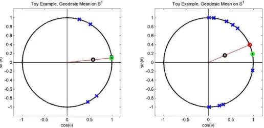
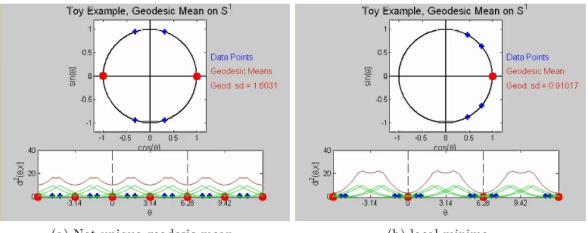
5.3.2 Examples: Geodesic Means on Various Manifolds . . . 80
5.4 Backward Generalization of PCA on manifolds . . . 87
6 Principal Arc Analysis on direct product manifold . . . 91
6.1 Introduction . . . 91
6.2 Circle class for non-geodesic variation onS2 . . . . 94
6.3 Suppressing small least-squares circles . . . 99
6.4 Principal Arc Analysis on direct product manifolds . . . 106
6.5 Application to m-rep data . . . 111
6.5.1 The Medial Representation of prostate . . . 111
6.5.2 Simulated m-rep object . . . 112
6.5.3 Prostate m-reps from real patients . . . 113
6.6 Doubly iterative algorithm to find the least-squares small circle . . . 114
7 Analysis of Principal Nested Spheres . . . 119
7.1 Introduction . . . 119
7.2 Principal Nested Spheres . . . 122
7.2.1 Geometry of Nested Spheres . . . 122
7.2.2 The Best Fitting Subsphere . . . 124
7.2.3 The sequence of Principal Nested Spheres . . . 124
7.2.4 Euclidean-type representation . . . 125
7.2.5 Principal Arcs . . . 126
7.2.6 Principal Nested Spheres restricted to Great Spheres . . . 127
7.3 Visualization of nested spheres ofS3 . . . 128
7.4 Prevention of overfitting by sequential tests . . . 130
7.4.1 Likelihood ratio test . . . 130
7.4.2 Parametric bootstrap test . . . 131
7.4.3 Application procedure . . . 132
7.5 Computational Algorithm . . . 134
7.6 Application to Shape space . . . 136
7.6.1 Planar shape space . . . 136
7.6.2 Principal Nested Spheres for planar shapes . . . 137
7.6.3 Principal Nested Spheres for spaces of m >2 dimensional shapes . . . . 140
7.7 Real Data Analysis . . . 141
7.8 Geometry of Nested Spheres . . . 148
7.8.1 Preliminary Transformations: Rotation matrices . . . 148
7.8.2 Geometry of Subsphere . . . 149
7.9 Proofs and Additional Lemmas . . . 154
List of Figures
2.1 Example showing that PCA works in the HDLSS context . . . 10
2.2 Examples of theϵ-conditions . . . 17
2.3 Cartoon illustrates the consistency in HDLSS context . . . 20
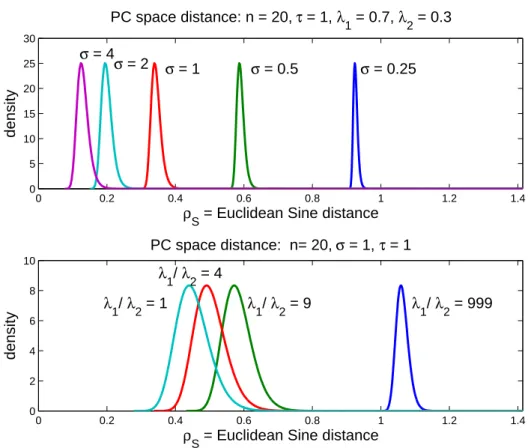
3.1 Density functions of the limiting distributions of the angle between u1 and ˆu1 . 45 3.2 The limiting distribution of the angles for them= 2 case . . . 55
3.3 Limiting distributions of the Euclidean sine distance . . . 56
3.4 The three different HDLSS geometric representations . . . 59
5.1 Extrinsic Mean and Intrinsic Mean on the circle . . . 79
5.2 Geodesic mean set on S1 . . . 82
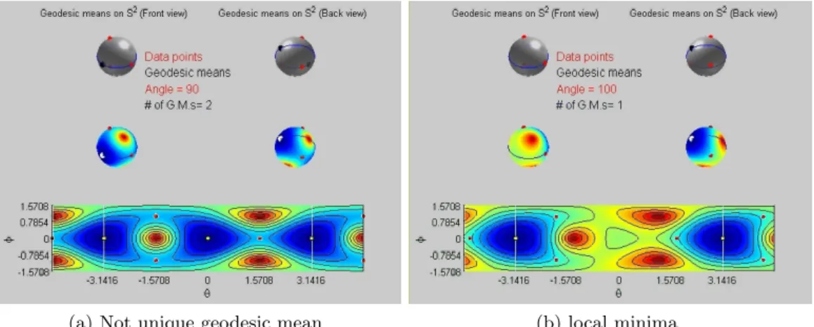
5.3 Geodesic mean set on S2 . . . 83
5.4 Geodesic mean set on S1×S1 . . . 85
5.5 Example of a geodesic mean on S2 . . . 85
5.6 Forward and Backward viewpoints of PCA . . . 88
6.1 S2-valued samples of the prostate m-reps . . . 93
6.2 Four generic distributions on a sphere . . . 97
6.3 Illustration of the signal+error model for a circle inS2 . . . 101
6.4 Overlaid target densities in suppressing small circles . . . 102
6.5 Simulation results for the estimation of the signal-to-noise ratio . . . 105
6.6 Illustration of the discontinuity between small and great circles . . . 107
6.7 The transformationhδ:S2 →R2 . . . 111
6.8 The prostate m-rep, revisited. . . 112
6.9 Scree plots and Scatter plots to compare PGA and PAA. . . 114
6.10 The first principal component arcs (geodesics) with data. . . 115
6.11 Scatter plots of PGA and PAA from real patients data. . . 115
7.2 Idea of PNS, illustrated. . . 123
7.3 Visualization of nested spheres. . . 129
7.4 Two different null hypothesis in prevention of overfitting of PNS. . . 131
7.5 Migration path of an elephant seal. . . 142
7.6 Scatterplots for sand grain data. . . 144
7.7 Sand grain configurations with sea and river groups. . . 144
7.8 Human movement data overlay. . . 145
7.9 Human movement data with fitted curves. . . 146
7.10 Rat skull growth data. . . 147
7.11 The first principal mode in rat skull growth data. . . 147
List of Tables
Chapter 1
Introduction
This dissertation demonstrates development, theoretical study, and implementation of
statis-tical methods for non-standard data, where conventional statisstatis-tical methods are sometimes
not directly applicable. The non-standard data are increasingly emerging, examples of which
are the data with High Dimension, Low Sample Size (HDLSS, or the large p, small n) and the data that naturally lie on curved manifolds. Specifically, datasets with those properties
are frequently observed in image and shape analysis, genomics, and functional data. These
application areas together span a new statistical field in which traditional concepts need to be
re-considered and development of new methodologies is required. The dissertation addresses
two important aspects of this broad field: The HDLSS asymptotics, where the limiting
opera-tion has the dimension growing with the sample size fixed, to understand the use of Principal
Component Analysis (PCA) in the HDLSS context; Development of PCA-like methods for
manifold data, where the proposed methods intuitively capture major non-linear variations in
lower dimension.
1.1
Motivations and Problems
The work is mainly motivated by statistical problems arising in image and shape analysis. The
image analysis concerns extraction of information from an image, or set of images, usually in a
digital form. The field of image analysis is broad, where mathematician, computer scientists,
engineers, medical researchers and statisticians have contributed in different aspects of the
area, separately or in collaborative fashion. Statistical image analysis puts a distributional
sta-tistical procedures to obtain meaningful information from the images. A subcategory of the
broad field concerns an object found in images (e.g. human brain from an image of MRI),
where the set of objects is under investigation. The statistical shape analysis focuses on the
objectshape in the image.
A shape can be represented by many different methods, examples of which are the
me-dial representations (Siddiqi and Pizer (2008)), a point correspondence model and spherical
harmonic representations (Gerig et al. (2004)), the traditional landmark-based shapes
(Book-stein (1991), Dryden and Mardia (1998)) and a newly developed functional representation
for shapes (Srivastava et al. (2010)). A challenge in shape analysis is that natural sample
spaces of those shape representations are usually not Euclidean spaces but curved manifolds.
In particular, the statistical methods that benefit from Euclidean geometry are not directly
applicable for the manifold-valued objects. This motivates statistical study of manifold-valued
random variables.
Another challenge in the image analysis is that the dimensionality of the representations
is very high. Due to advances in modern technology, obtaining high resolution images became
easier. However, the sample size (i.e. the number of observations) stays low especially in the
medical image analysis because of the high cost in obtaining medical images such as MRI and
CT. Hall et al. (2005) termed the situation as High Dimension, Low Sample Size (HDLSS)
context, which becomes increasingly common and is observed not only in medical imaging but
also in genomics, chemometrics, and functional analysis.
In the broad field of image analysis, we focus on data analyses in the sample space of the
representations, called feature space. Specifically, we wish to give insight into the following
basic statistical tasks:
1. Exploratory statistics and visualization of important structure: Given a random object
or a set of observations of those in a non-Euclidean and multi-dimensional feature space,
the first task for a statistician is to provide exploratory statistics. This includes finding
a central location (mean), measure of variability (variance), and patterns in the data
set.
wish to find an affine subspace of smaller dimension in a way that we do not lose
important variation. If the feature space is a non-Euclidean curved manifold, we wish
to find a sub-manifold of smaller dimension with great variance contained.
3. Estimation of probability distribution: A probability distribution can be assumed with
fewer parameters if we choose to work with the subspace (or the sub-manifold) found in
the dimension reduction.
The Principal Component Analysis (PCA) plays an important role in all of those problems.
PCA is often used in multivariate analysis for dimension reduction and visualization of
important modes of variation. It is also understood as an estimation of the population
princi-pal components by the sample principrinci-pal components. PCA is commonly credited to Hotelling
(1933) and its common references are Muirhead (1982) and Jolliffe (2002). The objective of
PCA is to capture most of the variability, of a multidimensional random vector or a set of
observations consisting of a large number of measurements, in a low dimensional subspace.
When the sample space is a Euclidean (linear) space, PCA finds a sequence of affine subspaces
or a set of orthogonal direction vectors. Optimal choice of this sequence can be characterized
in two equivalent ways: maximization of the variance captured by the affine subspace or
min-imization of the variance of the residuals. In the Euclidean space, PCA is usually computed
through the eigen-decomposition of covariance matrices.
We discuss two different views of the PCA, namely the forward and backward stepwise
views, later in Part II of the dissertation. These views are first introduced in Marron et al.
(2010), which stems from the work in this dissertation.
Now, consider using PCA in the image or shape analysis, which in fact is a common routine
for data analysts. While the traditional PCA is well defined for random vectors, we have two
concerns; First of all, the sample size is usually too low but the dimension of the sample space
is very high; Second, the natural sample space of the features of images or shapes is not the
flat Euclidean space, but a curved manifold. A simple application of Euclidean PCA usually
fails in the case. There are two different but related research questions:
1. What is the behavior of PCA in the high dimension low sample size context?
Part I and II of the dissertation answer the first and second questions, respectively. A
short summary is given in the next section.
1.2
Summary and Contributions
In Part I of the dissertation, Euclidean PCA is asymptotically studied when the dimensiond
grows, while the sample sizenis fixed. In particular, we are interested in the situations when the PCA works in the HDLSS situation and when it fails. The success and failure of PCA are
well described by the consistency of the empirical Principal Component (PC) directions ˆui (or
theith eigenvector of the covariance matrix, see Section 2.1) with its population counterpart
ui, under the limiting operation d→ ∞ and n fixed. Since the size of the direction vectors
ui,uˆi are increasing asdgrows, the discrepancy between directions is measured by the angle
formed by the directions. We say ˆui is :
• consistent withui if Angle(ˆui, ui)→0 as d→ ∞;
• strongly inconsistent with ui if Angle(ˆui, ui)→π/2 as d→ ∞.
While the consistency is the case we desire, the strong inconsistency is somewhat
counterin-tuitive since the angle π/2 is indeed the largest possible value of the angle. In other words, the estimate ˆui of ui loses its connection to the population structure and becomes completely
arbitrary. We see that in HDLSS asymptotics when ˆui is not consistent, it is often not just
inconsistent but strongly inconsistent. The mathematical mechanism of these situations is the
main topic of Chapter 2. In short, when the population PC variance is large such as of order
dα, α >1, the corresponding PC direction estimate is consistent. If not so large, i.e. α <1, then the corresponding PC direction estimate is strongly inconsistent.
The distributional assumptions in the study are general and intuitive. Gaussianity is
relaxed into a ρ-mixing under some permutation and a moment condition. While the ρ -mixing assumption is most appropriate for a time series data set (because of the ordering
of the variables), we relax the assumption by allowing any permutation of variable ordering.
Thus the assumption makes sense for gene expression microarray data and image or shape
We also considered a case where PC directions are not distinguishable, which occurs when
some eigenvalues of the covariance matrix are identical. In Chapter 2, we consider a
sub-space spanned by those indistinguishable PC directions, and develop a notion of subsub-space
consistency.
A natural question arises after we see that the exponent α in the order of PC variance
dα is the main driver between consistency (α >1) and strong inconsistency (α <1). What can we expect at the boundary between two cases? Chapter 3 discusses topics related to this
question. We find that the angles do not degenerate (either to 0 orπ/2) but weakly converge to distributions with support in (0, π/2). We provide explicit forms of the limiting distributions in Sections 3.2 and 3.3. We further extend the HDLSS geometric representation (i.e. modulo
rotation, n independent samples converge to vertices of a regular n simplex) found in Hall et al. (2005) and Ahn et al. (2007) intothree different HDLSS representations, which gives an
intuition in understanding a transition between consistency and strong inconsistency.
Part I of the dissertation is concluded with a discussion on open problems and a literature
review; see Chapter 4.
The second part of the dissertation introduces some developments in generalization of
PCA to manifold-valued data. We begin by introducing examples of specific manifolds, that
are feature spaces in image analysis (Section 5.1). This gives a motivation to focus on specific
types of manifolds. We briefly describe some basic Riemannian geometry used in the analysis
and some specific manifolds we focus in Section 5.2. In particular, we focus on spheres and
direct product of those with Euclidean space.
A common goal in analyzing these manifold data is to understand the variability. PCA,
when appropriately modified and implemented for manifolds, provides a very effective means
of analyzing the major modes of variation. The main contribution of Part II is to provide
flexible extensions of PCA to manifold data. Briefly, the main idea in improving PCA is to
make the method adaptive to certain non-linear structures of the data while the desirable
properties of PCA are inherited.
To elaborate the work intuitively, let us assume that the manifold is the usual unit sphere
a great circle. As in the standard PCA, one may find a mean first then fit a great circle as
the first PC direction. The second and higher PC directions are found among all great circles
orthogonal to the first PC (geodesic). However, we found out that this standard approach may
lead to an ineffective representation of the data, as discussed in Section 6.2. To resolve this
issue, we took a reverse viewpoint in generalizing PCA, calledbackward approach, where the
dimensionality of approximating subspaces (or submanifolds) is successively reduced. That
is, analogous to the backward variable selection in regression, we remove the least important
component first. This backward approach agrees with the standard PCA in Euclidean space
but not in manifolds. The backward stepwise viewpoint gives a common root in generalization
of PCA to non-linear spaces. In Section 5.4 the two different viewpoints of the usual PCA is
discussed, and we point out that the backward approach is suitable for extension of PCA to
manifold data.
The backward approach not only works well when the standard approach fails, but also
gives a flexibility in capturing variations. The generalized PCA by the backward approach
can be relaxed to find a small circle (e.g. the Tropic of Cancer) of the sphere, adaptive to the
data. The resulting principal arcs capture the variation in the data set more succinctly and
serve as principal components for visualization and dimension reduction.
The two methods proposed in Part II are generalizations of PCA to manifold-valued
vari-ables. Chapter 6 discusses Principal Arc Analysis for direct product manifolds; Chapter
7 discusses Analysis of Principal Nested Spheres for hyperspheres and the shape spaces of
Kendall (1984).
The direct product manifold is a class of specially structured manifolds. The sample
spaces of medial shape representations, diffeomorphisms, point distribution models, points
and normals models and size-and-shapes can all be considered as a special form of direct
product manifolds. We propose to use a transformation of non-Euclidean data into Euclidean
coordinates, then a composite space of Euclidean data and the transformed non-Euclidean
data gives a space suitable for further analysis including non-linear dimension reduction,
visualization, and modeling with fewer parameters. Principal Arc Analysis consists of 1)
estimation of the principal circle, which is the basis for transformations, 2) choices of the
discusses an application of Principal Arc Analysis to medial shape representations data set.
Analysis of Principal Nested Spheres can be viewed as an extension of Principal Arc
Analysis to higher dimensional spheresSdand Kendall’s shape space. Since the dimension of the sphere is now higher than the simple 2, the geometry involved is a bit more complicated
than the usual sphere. We define nested spheres, which are in a special form of sub-manifolds of
Sd, as a basis for decomposition of the hypersphere. Geometry of nested spheres are discussed
in depth in Section 7.8. Simply put, Principal Nested Spheres are fitted nested spheres that
capture most of the variances in the data. We discuss application of Analysis of Principal
Nested Spheres to Kendall’s shape space in Section 7.6, as well as several real data examples
in Section 7.7. We exemplify that the proposed method results in a succinct description of
Part I
Chapter 2
PCA consistency in HDLSS context
Since traditional tools of multivariate statistical analysis were designed for then > d case, it should not be surprising that they often do not work properly for the HDLSS data. However,
the method of PCA has been seen to sometimes be very effective in the HDLSS context, and is
widely used as a dimension reduction technique. In this chapter we investigate the asymptotic
behaviors of PCA when d tends to infinity while n is fixed, which provide the appropriate analysis to study the HDLSS context. In short, the asymptotics characterizes when Euclidean
PCA works and when it fails. The work presented in this chapter is based on Jung and Marron
(2009).
2.1
Introduction and summary
The High Dimension, Low Sample Size (HDLSS) data situation occurs in many areas of
modern science and the asymptotic studies of this type of data are becoming increasingly
relevant. We will focus on the case that the dimension dincreases while the sample size nis fixed as done in Hall et al. (2005) and Ahn et al. (2007). Thed-dimensional covariance matrix is challenging to analyze in general since the number of parameters is d(d2+1), which increases even faster thand. Instead of assessing all of the parameter estimates, the covariance matrix is usually analyzed by Principal Component Analysis (PCA). PCA is often used to visualize
important structure in the data, as shown in Figure 2.1. The data in Figure 1, described in
detail in Bhattacharjee et al. (2001) and Liu et al. (2008), are from a microarray study of lung
cancer. Different symbols correspond to cancer subtypes and Figure 2.1 shows the projections
−20 0 20 40 −20
0 20 40
PC 2
PC 1
−40 −20 0 20
−20 0 20 40
PC 3
PC 1
Figure 2.1: Scatterplots of data projected on the first three PC directions. The dataset contains 56 patients with 2530 genes. There are 20 Pulmonary Carcinoid (plotted as +), 13 Colon Cancer Metastases (∗), 17 Normal Lung (◦), and 6 Small Cell Carcinoma (×). In spite of the high dimensionality, PCA reveals important structure in the data.
(right panel, respectively) directions. This shows the difference between subtypes is so strong
that it drives the first three principal components. This illustrates common occurrence: the
data have important underlying structure which is revealed by the first few PC directions.
PCA is also used to reduce dimensionality by approximating the data with the first few
principal components.
For both visualization and data reduction, it is critical that the PCA empirical
eigenvec-tors reflect true underlying distributional structure. Hence our focus is on the underlying
mechanism which determines when the sample PC directions converge to their population
counterparts as d → ∞. For example, we quantify situations where the dominant sample eigenvectors are revealing important underlying structure in the data as in Figure 2.1. In
gen-eral we assume d > n. Since the size of the covariance matrix depends on d, the population covariance matrix is denoted as Σd and similarly the sample covariance matrix, Sd, so that
their dependency on the dimension is emphasized. PCA is done by eigen-decomposition of a
covariance matrix. The eigen-decomposition of Σd is
where Λd is a diagonal matrix of eigenvalues λ1,d > λ2,d > · · · >λd,d and Ud is a matrix of
corresponding eigenvectors so thatUd= [u1,d, u2,d, . . . , ud,d]. Sd is similarly decomposed as
Sd= ˆUdΛˆdUˆd′.
Ahn et al. (2007) developed the concept of HDLSS consistency which was the first
inves-tigation of when PCA could be expected to find important structure in HDLSS data. Our
main results are formulated in terms of three related concepts:
1. consistency: The direction ˆui,d is consistent with its population counterpart ui,d if
Angle(ui,d,uˆi,d) −→ 0 as d → ∞. The growth of dimension can be understood as
adding more variation. The consistency of sample eigenvectors occurs when the added
variation supports the existing structure in the covariance or is small enough to be
ignored.
2. strong inconsistency: In situations where ˆui,d is not consistent, a perhaps
counter-intuitive HDLSS phenomenon frequently occurs. In particular, ˆui,dis said to bestrongly
inconsistent with its population counterpart ui,d in the sense that it tends to be as
far away from ui,d as possible, that is, Angle(ui,d,uˆi,d) −→ π2 as d → ∞. Strong
in-consistency occurs when the added variation obscures the underlying structure of the
population covariance matrix.
3. subspace consistency: When several population eigenvalues indexed byj∈J are similar, the corresponding sample eigenvectors may not be distinguishable. In this case, ˆuj,d will
not be consistent foruj,d but will tend to lie in the linear span, span{uj,d:j∈J}. This
motivates the definition of convergence of a direction ˆui,d to a subspace, calledsubspace
consistency;
Angle(ˆui,d,span{uj,d :j∈J})−→0
as d → ∞. This definition essentially comes from the theory of canonical angles dis-cussed by Gaydos (2008). That theory also gives a notion of convergence of subspaces,
that could be developed here.
inconsis-tency are provided. Section 2.2 develops conditions that guarantee the non-zero eigenvalues
of the sample covariance matrix tend to a increasing constant, which are much more general
than those of Hall et al. (2005) and Ahn et al. (2007). This asymptotic behavior of the sample
covariance matrix is the basis of the geometric representation of HDLSS data. Our result
gives broad new insight into this representation as discussed in section 2.3. The central issue
of consistency and strong inconsistency is developed in section 2.4, as a series of theorems.
For a fixed number κ, we assume the firstκ eigenvalues are much larger than the others. We show that when κ= 1, the first sample eigenvector is consistent and the others are strongly inconsistent. We also generalize to the κ > 1 case, featuring two different types of results (consistency and subspace consistency) according to the asymptotic behaviors of the first κ
eigenvalues. All results are combined and generalized in the main theorem (Theorem 2.5).
Proofs of theorems are given in section 2.5.
Further discussions on the boundary case where the PC directions are neither consistent
nor strongly inconsistent are deferred to Chapter 3. Relevant literatures are reviewed and
discussed later at Chapter 4.
2.1.1 General setting
Suppose we have a d×n data matrix X(d) = [X1,(d), . . . , Xn,(d)] with d > n, where the
d-dimensional random vectors X1,(d), . . . , Xn,(d) are independent and identically distributed.
We assume that each Xi,(d) follows a multivariate distribution (which does not have to be
Gaussian) with mean zero and covariance matrix Σd. Define the sphered data matrixZ(d)=
Λ−d1/2Ud′X(d). Then the components of the d×n matrix Z(d) have unit variances, and are
uncorrelated with each other. We shall regulate the dependency (recall for non-Gaussian data,
uncorrelated variables can still be dependent) of the random variables inZ(d) by a ρ-mixing condition. This allows serious weakening of the assumptions of Gaussianity while still enabling
the law of large numbers that lie behind the geometric representation results of Hall et al.
(2005).
L2(A) denote the space of square-integrable, A measurable (real-valued) random variables.
For eachm>1, define the maximal correlation coefficient
ρ(m) := sup|corr(f, g)|, f ∈L2(F−∞j ), g∈L2(Fj∞+m),
where sup is over all f,g and j ∈Z. The sequence {Zi} is said to be ρ-mixing if ρ(m)→ 0
asm→ ∞.
While the concept ofρ-mixing is useful as a mild condition for the development of laws of large numbers, its formulation is critically dependent on the ordering of variables. For many
interesting data types, such as microarray data, there is clear dependence but no natural
ordering of the variables. Hence we assume that there is some permutation of the data which
isρ-mixing. In particular, let{Zij,(d)}id=1 be the components of thejth column vector ofZ(d).
We assume that for eachd, there exists a permutation πd :{1, . . . , d} 7−→ {1, . . . , d} so that
the sequence{Zπd(i)j,(d) :i= 1, . . . , d} isρ-mixing.
In the following, all the quantities depend on d, but the subscript d will be omitted for the sake of simplicity when it does not cause any confusion. The sample covariance matrix is
defined asS=n−1XX′. We do not subtract the sample mean vector because the population
mean is assumed to be 0. Since the dimension of the sample covariance matrix S grows, it is challenging to deal with S directly. A useful approach is to work with the dual of S. The dual approach switches the role of columns and rows of the data matrix, by replacing X by
X′. Then×n dual sample covariance matrix is defined asSD =n−1X′X. An advantage of
this dual approach is thatSD andS share non-zero eigenvalues. If we write X asUΛ
1 2Z and use the fact thatU is a unitary matrix,
nSD = (Z′Λ
1
2U′)(UΛ 1
2Z) =Z′ΛZ =
d
∑
i=1
λi,dzi′zi, (2.1)
where thezi’s,i= 1, . . . , d, are the row vectors of the matrix Z. Note thatnSD is commonly
2.2
HDLSS asymptotic behavior of the sample covariance
ma-trix
In this section, we investigate the behavior of the sample covariance matrix S when d→ ∞
andnis fixed. Under mild and broad conditions, the eigenvalues ofS, or the dualSD, behave
asymptotically as if they are from the identity matrix. That is, the set of sample eigenvectors
tends to be an arbitrary choice. This lies at the heart of the geometric representation results
of Hall et al. (2005) and Ahn et al. (2007) which are studied more deeply in section 2.3. We
will see that this condition readily implies the strong inconsistency of sample eigenvectors, see
Theorem 2.5.
The conditions for the theorem are conveniently formulated in terms of a measure of
sphericity
ϵ≡ tr
2(Σ)
dtr(Σ2) =
(∑di=1λi,d)2
d∑di=1λ2
i,d
,
proposed and used by John (1971, 1972) as the basis of a hypothesis test for equality of
eigenvalues. Note that these inequalities always hold:
1
d 6ϵ61.
Also note that perfect sphericity of the distribution (i.e. equality of eigenvalues) occurs only
when ϵ= 1. The other end of theϵ range is the most singular case where in the limit as the first eigenvalue dominates all others.
Ahn et al. (2007) claimed that ifϵ≫ 1d, in the sense thatϵ−1=o(d), then the eigenvalues of SD tend to be identical in probability as d → ∞. However, they needed an additional
assumption (e.g. a Gaussian assumption on X(d)) to have independence among components ofZ(d), as described in example 2.1. We extend this result to the case of arbitrary distributions with dependency regulated by theρ-mixing condition as in section 2.1.1, which is much more general than either a Gaussian or an independence assumption. We also explore convergence
in the almost sure sense with stronger assumptions. Our results use a measure of sphericity for
In particular, define the measure of sphericity for{λk,d, . . . , λd,d} as
ϵk ≡
(∑di=kλi,d)2
d∑di=kλ2
i,d
.
For convenience, we name several assumptions used in this chapter made about the measure
of sphericityϵ:
• Theϵ-condition: ϵ≫ d1, i.e.
(dϵ)−1 = ∑d
i=1λ2i,d
(∑di=1λi,d)2
→0 as d→ ∞. (2.2)
• Theϵk-condition: ϵk≫ 1d, i.e.
(dϵk)−1=
∑d i=kλ2i,d
(∑di=kλi,d)2
→0 as d→ ∞. (2.3)
• The strongϵk-condition: For some fixedl>k,ϵl≫ √1d, i.e.
d−12ϵ−1
l =
d12 ∑d
i=lλ2i,d
(∑di=lλi,d)2
→0 as d→ ∞. (2.4)
Remark 2.1. Note that theϵk-condition is identical to theϵ-condition when k= 1. Similarly,
the strong ϵk-condition is also called the strong ϵ-condition when k = 1. The strong ϵk
-condition is stronger than theϵk condition if the minimum of l’s which satisfy (2.4), lo, is as
small ask. But, iflo > k, then this is not necessarily true. We will use the strongϵk-condition
combined with the ϵk-condition.
Note that the ϵ-condition is quite broad in the spectrum of possible values of ϵ: It only avoids the most singular case. The strong ϵ-condition further restrictsϵl to essentially in the
range (√1
d,1].
The following theorem states that if the (strong)ϵ-condition holds for Σd, then the sample
eigenvalues behave as if they are from a scaled identity matrix. It uses the notationInfor the
Theorem 2.1. For a fixedn, letΣd=UdΛdUd′,d=n+1, n+2, . . .be a sequence of covariance
matrices. Let X(d) be a d×n data matrix from a d-variate distribution with mean zero and covariance matrixΣd. LetSd= ˆUdΛˆdUˆd′ be the sample covariance matrix estimated fromX(d) for each dand let SD,d be its dual.
(1) Assume that the components of Z(d) = Λ
−1 2
d Ud′X(d) have uniformly bounded fourth moments and areρ-mixing under some permutation. If (2.2) holds, then
c−d1SD,d−→In, (2.5)
in probability as d→ ∞, where cd=n−1
∑d i=1λi,d.
(2) Assume that the components of Z(d) = Λ− 1 2
d Ud′X(d) have uniformly bounded eighth moments and are independent to each other. If both (2.2) and (2.4) hold, thenc−d1SD,d→In
almost surely as d→ ∞.
The (strong)ϵ-condition holds for quite general settings. The strongϵ-condition combined with theϵ-condition holds under;
(a) Null case: All eigenvalues are the same.
(b) Mild spiked model: The first m eigenvalues are moderately larger than the others, for example,λ1,d=· · ·=λm,d =C1·dα and λm+1,d=· · ·=λd,d=C2, wherem < d,α <1
and C1, C2 >0.
Theϵ-condition fails when;
(c) Singular case: Only the first few eigenvalues are non-zero.
(d) Exponential decrease: λi,d =c−i for somec >1.
(e) Sharp spiked model: The first m eigenvalues are much larger than the others. One example is the same as (b) butα>1.
The polynomially decreasing case, λi,d = i−β, is interesting because it depends on the
power β;
Figure 2.2: Theϵ-condition is satisfied by the mild spike and polynomial decrease case, but is satisfied by the exponential decrease.
(f-2) The ϵ-condition holds but the strong ϵ-condition fails when 34 6β 61.
(f-3) The ϵ-condition fails whenβ >1.
Another family of examples that includes all three cases is the spiked model with the
number of spikes increasing, for example, λ1,d = · · · = λm,d = C1·dα and λm+1,d = · · · =
λd,d=C2, where m=⌊dβ⌋, 0< β <1 and C1, C2>0;
(g-1) The strong ϵ-condition holds when 062α+β < 32;
(g-2) The ϵ-condition holds but the strong ϵ-condition fails when 32 62α+β <2;
(g-3) The ϵ-condition fails when 2α+β >2.
Figure 2.2 shows some examples depicting when the ϵ-condition holds and fails.
2.3
Geometric representation of HDLSS data
Suppose X ∼ Nd(0, Id). When the dimension d is small, most of the mass of the data lies
near origin. However with a large d, Hall et al. (2005) showed that Euclidean distance ofX
to the origin is described as
∥X∥=√d+op(
√
Moreover the distance between two samples is also rather deterministic, i.e.
∥X1−X2∥= √
2d+op(
√
d). (2.7)
These results can be derived by the law of large numbers. Hall et al. (2005) generalized those
results under the assumptions thatd−1∑di=1Var(Xi)→1 and{Xi} isρ-mixing.
Application of part (1) of Theorem 2.1 generalizes these results. Let X1,(d), X2,(d) be
two samples that satisfy the assumptions of Theorem 2.1 part (1). Assume without loss of
generality that limd→∞d−1
∑d
i=1λi,d = 1. The scaled squared distance between two data
points is
∥X1,(d)−X2,(d)∥2
∑d i=1λi,d
=
d
∑
i=1
˜
λi,dzi21+
d
∑
i=1
˜
λi,dzi22−2
d
∑
i=1
˜
λi,dzi1zi2,
where ˜λi,d= λi,d
∑d i=1λi,d
. Note that by (2.1), the first two terms are diagonal elements ofc−d1SD,d
in Theorem 2.1 and the third term is an off-diagonal element. Sincec−d1SD,d → In, we have
(2.7). (2.6) is derived similarly.
Remark 2.2. If limd→∞d−1
∑d
i=1λi,d = 1, then the conclusion (2.5) of Theorem 2.1 part (1)
holds if and only if the representations (2.6) and (2.7) hold under the same assumptions in
the theorem.
In this representation, theρ-mixing assumption plays a very important role. The following example, due to John Kent, shows that some type of mixing condition is important.
Example2.1 (Strong dependency via a scale mixture of Gaussian). LetX =Y1U+σY2(1−U),
whereY1,Y2 are two independent Nd(0, Id) random variables, U = 0 or 1 with probability 12
and independent ofY1,Y2, and σ >1. Then,
∥X∥=
d12 +Op(1) w.p. 1
2
σd12 +Op(1) w.p. 1
2
Thus, (2.6) does not hold. Note that since Cov(X) = 1+2σ2Id, the ϵ-condition holds and
under Gaussian assumption, given any covariance matrix Σ, Z = Σ−12X has independent components.
Note that in the caseX = (X1, . . . , Xd) is a sequence of i.i.d. random variables, the results
(2.6) and (2.7) can be considerably strengthened to ∥X∥ = √d+Op(1), and ∥X1−X2∥ = √
2d+Op(1). The following example shows that strong results are beyond the reach of
reasonable assumption.
Example 2.2 (Varying sphericity). Let X ∼ Nd(0,Σd), where Σd = diag(dα,1, . . . ,1) and
α ∈ (0,1). Define Z = Σ− 1 2
d X. Then the components of Z, zi’s, are independent standard
Gaussian random variables. We get∥X∥2=dαz12+∑di=2zi2. Now for 0< α < 12,d−12(∥X∥2−
d) ⇒ N(0,1) and for 12 < α < 1, d−α(∥X∥2 −d) ⇒ z12, where ⇒ denotes convergence in distribution. Thus by the delta-method, we get
∥X∥=
√
d+Op(1), if 0< α < 12,
√
d+Op(dα−
1
2), if 1
2 < α <1.
In both cases, the representation (2.6) holds.
2.4
Consistency and strong inconsistency of PC directions
In this section, conditions for consistency or strong inconsistency of the sample PC direction
vectors are investigated, in the general setting of section 2.1.1. The generic eigen-structure
of the covariance matrix that we assume is the following. For a fixed number κ, we assume the first κ eigenvalues are much larger than others. (The precise meaning of large will be addressed shortly.) The rest of eigenvalues are assumed to satisfy the ϵ-condition, which is very broad in the range of sphericity. We begin with the caseκ= 1 and generalize the result forκ >1 in two distinct ways. The main theorem (Theorem 2.5) contains and combines those previous results and also embraces various cases according to the magnitude of the first κ
eigenvalues. We also investigate the sufficient conditions for a stronger result, i.e. almost sure
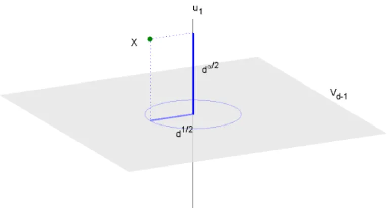
Figure 2.3: Projection of a d-dimensional random variable X ontou1 and Vd−1. Ifα > 1, then the
subspaceVd−1becomes negligible compared tou1 whend→ ∞
2.4.1 Criteria for consistency or strong inconsistency of the first PC
direc-tion
Consider the simplest case that only the first PC direction of S is of interest. Section 2.3 gives some preliminary indication of this. As an illustration, consider a spiked model as in
Example 2.2 but now let α > 1. Let {ui} be the set of eigenvectors of Σd and Vd−1 be the
subspace of all eigenvectors except the first one. Then the projection of X onto u1 has a
norm∥Proju1X∥=∥X1∥=Op(d
α
2). The projection ofX onto Vd−1 has a norm
√
d+op(
√
d) by (2.6). Thus when α > 1, if we scale the whole data space Rd by dividing by dα2, then ProjVd−1X becomes negligible compared to Proju1X. (See Figure 2.3.) Thus for a large d, Σd ≈ λ1u1u′1 and the variation of X is mostly along u1. Therefore the sample eigenvector
corresponding to the largest eigenvalue, ˆu1, will be similar tou1.
To generalize this, suppose the ϵ2 condition holds. The following proposition states that
under the general setting in section 2.1.1, the first sample eigenvector ˆu1 converges to its
pop-ulation counterpartu1 (consistency) or tends to be perpendicular tou1 (strong inconsistency)
according to the magnitude of the first eigenvalueλ1, while all the other sample eigenvectors
are strongly inconsistent regardless of the magnitude λ1.
Proposition 2.2. For a fixed n, let Σd = UdΛdUd′, d = n+ 1, n+ 2, . . . be a sequence of
covariance matrices. Let X(d) be a d×n data matrix from a d-variate distribution with mean zero and covariance matrix Σd. Let Sd= ˆUdΛˆdUˆd′ be the sample covariance matrix estimated
(a) The components of Z(d)= Λ
−1 2
d Ud′X(d) have uniformly bounded fourth moments and are
ρ-mixing for some permutation.
For an α1 >0,
(b) λ1,d
dα1 −→c1 for some c1 >0,
(c) Theϵ2-condition holds and
∑d
i=2λi,d =O(d).
If α1 >1, then the first sample eigenvector is consistent and the others are strongly inconsis-tent in the sense that
Angle(ˆu1, u1)
p
−→0 asd→ ∞,
Angle(ˆui, ui) p
−→ π
2 as d→ ∞ ∀i= 2, . . . , n.
If α1∈(0,1), then all sample eigenvectors are strongly inconsistent, i.e.
Angle(ˆui, ui) p
−→ π
2 as d→ ∞ ∀i= 1, . . . , n.
Note that the gap between consistency and strong inconsistency is very thin, i.e. if we
avoid α1 = 1, then we have either consistency or strong inconsistency. Thus in the HDLSS
context, asymptotic behavior of PC directions is mostly captured by consistency and strong
inconsistency. Now it makes sense to say λ1 is much larger than the others when α1 > 1,
which results in consistency. Also note that if α1 <1, then the ϵ-condition holds, which is in
fact the condition for Theorem 2.1.
2.4.2 Generalizations
In this section, we generalize Proposition 2.2 to the case that multiple eigenvalues are much
larger than the others. This leads to two different types of result.
First is the case that the first p eigenvectors are each consistent. Consider a covariance structure with multiple spikes, that is, p eigenvalues, p >1, which are much larger than the others. In order to have consistency of the first p eigenvectors, we require that each of p
eigenvalues has a distinct order of magnitude, for example, λ1,d =d3, λ2,d =d2 and sum of
Proposition 2.3. For a fixed n, let Σd, X(d), and Sd be as before. Assume (a) of
Propo-sition 2.2. Let α1 > α2 > · · · > αp > 1 for some p < n. Suppose the following conditions
hold:
(b) λi,d
dαi −→ci for some ci >0, ∀i= 1, . . . , p
(c) Theϵp+1-condition holds and
∑d
i=p+1λi,d =O(d).
Then, the firstpsample eigenvectors are consistent and the others are strongly inconsistent in the sense that
Angle(ˆui, ui) p
−→0 as d→ ∞ ∀i= 1, . . . , p,
Angle(ˆui, ui) p
−→ π
2 as d→ ∞ ∀i=p+ 1, . . . , n.
Consider now a distribution having a covariance structure with multiple spikes as before.
Letkbe the number of spikes. An interesting phenomenon happens when the firstk eigenval-ues are of the same order of magnitude, i.e. limd→∞ λλ1,d
k,d =c >1 for some constant c. Then the first k sample eigenvectors are neither consistent nor strongly inconsistent. However, all of those random directions converge to the subspace spanned by the firstkpopulation eigen-vectors. Essentially, when eigenvalues are of the same order, the eigen-directions can not be
separated but are subspace consistent with the proper subspace.
Proposition 2.4. For a fixed n, let Σd, X(d), and Sd be as before. Assume (a) of
Proposi-tion 2.2. Letα1>1 andk < n. Suppose the following conditions hold:
(b) λi,d
dα1 −→ci for some ci >0, ∀i= 1, . . . , k
(c) Theϵk+1-condition holds and
∑d
i=k+1λi,d =O(d).
Then, the first ksample eigenvectors are subspace-consistent with the subspace spanned by the first k population eigenvectors and the others are strongly inconsistent in the sense that
Angle(ˆui,span{u1, . . . , uk}) p
−→0 as d→ ∞ ∀i= 1, . . . , k,
Angle(ˆui, ui) p
−→ π
2.4.3 Main theorem
Propositions 2.2 - 2.4 are combined and generalized in the main theorem. Considerp groups of eigenvalues, which grow at the same rate within each group as in Proposition 2.4. Each
group has a finite number of eigenvalues and the number of eigenvalues in all groups,κ, does not exceedn. Also similar to Proposition 2.3, let the orders of magnitude of the pgroups be different to each other. We require that theϵκ+1-condition holds. The following theorem states
that a sample eigenvector of a group converges to the subspace of population eigenvectors of
the group.
Theorem 2.5 (Main theorem). For a fixed n, let Σd, X(d), andSd be as before. Assume (a)
of Proposition 2.2. Let α1, . . . , αp be such thatα1 > α2 >· · · > αp >1 for some p < n. Let
k1, . . . , kp be nonnegative integers such that
∑p j=1kj
.
=κ < n. Let k0 = 0 and kp+1 =d−κ. Let J1, . . . , Jp+1 be sets of indices such that
Jl =
l−1
∑
j=0
kj + 1, l−1
∑
j=0
kj+ 2, . . . , l−1
∑
j=0
kj+kl
, l= 1, . . . , p+ 1.
Suppose the following conditions hold:
(b) λi,d
dαl −→ci for some ci >0, ∀i∈Jl, ∀l= 1, . . . , p
(c) Theϵκ+1-condition holds and
∑
i∈Jp+1λi,d=O(d).
Then, the sample eigenvectors whose label is in the group Jl, for l = 1, . . . , p, are
subspace-consistent with the space spanned by the population eigenvectors whose labels are inJl and the
others are strongly inconsistent in the sense that
Angle(ˆui,span{uj :j∈Jl}) p
−→0 as d→ ∞ ∀i∈Jl, ∀l= 1, . . . p, (2.8)
and
Angle(ˆui, ui) p
−→ π
2 as d→ ∞ ∀i=κ+ 1, . . . , n. (2.9)
Remark 2.3. If the cardinality ofJl,kl, is 1, then (2.8) implies ˆui is consistent for i∈Jl.
Remark 2.4. The strongly inconsistent eigenvectors whose labels are inJp+1 can be considered
whose labels are in Jp+1 for each d, i.e. Γd = span{uj : j ∈ Jp+1} = span{uκ+1, . . . , ud}.
Then
Angle(ˆui,d,Γd) p
−→0 as d→ ∞,
for all i∈Jp+1.
Note that the formulation of the theorem is similar to the spiked covariance model but
much more general. The uniform assumption on the underlying eigenvalues, i.e. λi = 1 for
all i > κ, is relaxed to the ϵ-condition. We also have catalogued a large collection of specific results according to the various sizes of spikes.
These results are now illustrated for some classes of covariance matrices that are of special
interest. These covariance matrices are easily represented in factor form, i.e. in terms of
Fd= Σ
1 2
d.
Example 2.3. Consider a series of covariance matrices {Σd}d. Let Σd=FdFd′, where Fd is a
d×dsymmetric matrix such that
Fd= (1−ρd)Id+ρdJd=
1 ρd · · · ρd
ρd 1 . .. ...
..
. . .. ... ρd
ρd · · · ρd 1
,
where Jd is the d×d matrix of ones and ρd ∈ (0,1) depends on d. The eigenvalues of
Σd are λ1,d = (dρd+ 1−ρd)2, λ2,d = · · · = λd,d = (1−ρd)2. The first eigenvector is u1 = 1
√
d(1,1, . . . ,1)
′, while{u
2, . . . , ud}are any orthogonal sets of direction vectors perpendicular to
u1. Note that
∑d
i=2λi,d =d(1−ρd)2 =O(d) and theϵ2-condition holds. LetXd∼ Nd(0,Σd).
By Theorem 2.5, if ρd ∈(0,1) is a fixed constant or decreases to 0 slowly so that ρd≫d−
1 2,
then the first PC direction ˆu1is consistent. Else ifρddecreases to 0 so quickly thatρd≪d−
1 2,
then ˆu1 is strongly inconsistent. In both cases all the other sample PC directions are strongly
inconsistent.
diagonal matrix such that
Fd=
F1,d O
O F2,d
,
whereF1,d = (1−ρ1,d)Id+ρ1,dJdandF2,d= (1−ρ2,d)Id+ρ2,dJd. Suppose 0< ρ2,d 6ρ1,d<1.
Note that λ1,d = (dρ1,d+ 1−ρ1,d)2 , λ2,d = (dρ2,d+ 1−ρ2,d)2 and the ϵ3-condition holds.
Let X2d ∼ N2d(0,Σd). Application of Theorem 2.5 for various conditions on ρ1,d, ρ2,d is
summarized as follows. Denote, for two non-increasing sequencesµd,νd∈(0,1), µd≫νd for
νd=o(µd) andµd≽νd for limd→∞ µνdd =c∈[1,∞).
1. ρ1,d≫ρ2,d≫d−
1
2 : Both ˆu1,ˆu2 consistent.
2. ρ1,d≽ρ2,d ≫d−
1
2 : Both ˆu1,ˆu2 subspace-consistent to span{u1, u2}.
3. ρ1,d≫d−
1
2 ≫ρ2,d : ˆu1 consistent, ˆu2 strongly inconsistent. 4. d−12 ≫ρ1,d ≫ρ2,d : Both ˆu1,ˆu2 strongly inconsistent.
2.4.4 Corollaries to the main theorem
The result can be extended for special cases.
First of all, consider constructingX(d) fromZdbyX(d)≡UdΛ
1 2
dZdwhereZdis a truncated
set from an infinite sequence of independent random variables with mean zero and variance
1. This assumption makes it possible to have convergence in the almost sure sense. This is
mainly because the triangular array{Z1i,(d)}i,d becomes the single sequence{Z1i}i.
Corollary 2.6. Suppose all the assumptions in Theorem 2.5, with the assumption (a) replaced
by the following:
(a′) The components of Z(d) = Λ− 1 2
d Ud′X(d) have uniformly bounded eighth moments and are independent to each other. LetZ1i,(d) ≡Z1i for all i, d.
If the strong ϵκ+1-condition (2.4) holds, then the mode of convergence of (2.8) and (2.9) is almost sure.
have subspace consistency of ˆui with the proper subspace, which includes ui. Now letting
n→ ∞ makes it possible for ˆui to be consistent.
Corollary 2.7. Let Σd, X(d), and Sd be as before. Under the assumptions (a), (b) and (c) in
Theorem 2.5, assume further for (b) that the first κ eigenvalues are distinct, i.e. ci > cj for
i > j and i, j∈Jl for l= 1, . . . , p. Then for alli6κ,
Angle(ˆui, ui) p
−→0 as d→ ∞, n→ ∞, (2.10)
where the limits are applied successively.
If the assumption (a) is replaced by the assumption (a′) of Corollary 2.6, then the mode
of convergence of (2.10) is almost sure.
This corollary can be viewed as the case whend, ntend to infinity together, butdincreases at a much faster rate than n, i.e. d ≫ n. When n also increases in the particular setting of the corollary, the sample eigenvectors, which were only subspace-consistent in the d→ ∞
case, tend to be distinguishable and each of the eigenvectors is consistent. We conjecture that
the inconsistent sample eigenvalues are still strongly inconsistent whend, n→ ∞ and d≫n.
2.4.5 Limiting distributions of corresponding eigenvalues
The study of asymptotic behavior of the sample eigenvalues is an important part in the proof
of Theorem 2.5, and also could be of independent interest. The following lemma states that
the large sample eigenvalues increase at the same speed as their population counterpart and
the relatively small eigenvalues tend to be of order of d as d tends to infinity. Let φi(A)
denote the ith largest eigenvalue of the symmetric matrix A and φi,l(A) = φi∗(A) where
i∗ =i−∑lj−=11 kj.
Lemma 2.8. If the assumptions of Theorem 2.5 hold, and let Zl be a kl×n matrix from
blocks of Z as defined in (2.12), then
ˆ
λi/dαl =⇒ηi as d→ ∞ if i∈Jl, ∀l= 1, . . . , p,
ˆ
λi/d p
where each ηi is a random variable whose support is (0,∞) almost surely and indeed ηi =
φi,l(n−1C
1 2
l ZlZl′C
1
2)for eachi∈Jl, whereCl =diag{cj :j∈Jl}andK= limd→∞(dn)−1∑
i∈Jp+1λi,d.
If the data matrix X(d) is Gaussian, then the firstκ sample eigenvalues converge in
distri-bution to some quantities, which have known distridistri-butions.
Corollary 2.9. Under all the assumptions of Theorem 2.5, assume further that X(d) ∼
Nd(0,Σd) for each d. Then, for i∈Jl, l= 1, . . . p
ˆ
λi
dαl =⇒φi,l(n
−1W
kl(n, Cl)) as d→ ∞,
where Wkl(n, Cl) denotes akl×kl random matrix distributed as the Wishart distribution with
degree of freedomn and covariance Cl.
If kl= 1 for some l, then fori∈Jl
ˆ
λi
λi
=⇒ χ
2
n
n as d→ ∞,
where χ2n denotes a random variable distributed as the χ2 distribution with degree of freedom
n.
This generalizes the results in section 4.2 of Ahn et al. (2007).
2.5
Proofs
This section contains the proofs of theorems in this chapter.
Proof of Theorem 2.1. First we give the proof of part (1). By (2.1), the mth diagonal entry ofnSD can be expressed as
∑d
i=1λi,dzim,d2 wherezim,d is the (i, m)th entry of the matrixZ(d).
Define the relative eigenvalues ˜λi,d as ˜λi,d ≡ λi,d
∑d i=1λi,d
. Let πd denote the given permutation
for each dand let Yi =zπ2d(i)m,d−1. Then the Yi’s areρ-mixing, E(Yi) = 0 and E(Yi2) 6B
for allifor someB <∞. Letρ(m) = sup|corr(Yi, Yi+m)|where the sup is over alli. We shall