I. INTRODUCTION
A random walk with a step size distribution that has a divergent second moment is called a L´evy walk [1–3]. A L´evy
glassis a random medium where the separation between two scattering events has a divergent second moment. The term was coined by Barthelemy, Bertolotti, and Wiersma [4], for a random packing of polydisperse glass spheres. They measured the fractionT of the light intensity transmitted through such a random medium in a slab of thickness L, and found a power-law scalingT ∝1/Lγ with a superdiffusive exponent γ ≈0.5—intermediate between the values for ballistic motion (γ =0) and regular diffusion (γ =1).
The simplest theoretical description of propagation through a L´evy glass neglects correlations between subsequent scatter-ing events. The ray optics of the problem is then described by a L´evy walk, with a power-law step size distribution p(s)∝1/s1+α, 0< α <2. The experiment [4] was inter-preted in these terms, withα=1 andγ =α/2 the expected transmission exponent.
Correlations between scattering events in a L´evy glass dominate the dynamics in one dimension [5,6]. Although correlations were expected to become less significant with increasing dimensionality [7,8], Buonsante, Burioni, and Vezzani [9] have calculated that the transmission exponent γ should remain much larger than would follow from a L´evy walk with uncorrelated steps. In particular, a saturation at the diffusive valueγ =1 forα >1 is predicted—even though the second moment of the step size distribution becomes finite only forα >2.
To test these analytical predictions for the effect of correlations, we have simulated the transmission of classical particles through a L´evy glass, confined to a slab of thickness L. Both a two-dimensional (2D) system of disks is considered and a three-dimensional (3D) system of spheres. We find a power-law scalingT(L)∝1/Lγ with an exponentγthat lies well above the γ =α/2 line expected for a L´evy walk. In particular, we obtain a saturation ofγ at the diffusive value of unity well before theα=2 threshold is reached of a divergent second moment.
The outline of the paper is as follows. Since our aim is to compare the L´evy glass simulations with the predictions for a L´evy walk, we need analytical results for uncorrelated step sizes. These are summarized in the Appendix and referred to
in the main text. We start off in Sec.IIwith a description of the way in which we construct and simulate a L´evy glass on a computer. The results presented in that section are for 2D, where the largest systems can be studied. We turn to the 3D case in Sec. III and compare with the experiments [4]. We conclude in Sec.IV.
II. L ´EVY GLASS VERSUS L ´EVY WALK A. Construction
A L´evy glass [4,10] is a random packing of transparent spheres with a power-law distribution of radii,
n(r)∝1/r1+β. (2.1)
Light propagates without scattering (ballistically) through the spheres and diffusively (mean free path lmfp) in the region between the spheres. The probability to enter ad-dimensional sphere of radius betweenrandr+dr is proportional to the fraction n(r)dr of spheres in that size range, multiplied by the area∝rd−1. The ballistic segments (steps) of a ray inside a sphere of radius r have length s of order r. The sphere radius distribution (2.1) therefore corresponds to the step size distribution [11]
p(s)∝1/s1+α, with β =α+d−1. (2.2)
Particles propagating through a L´evy glass therefore have the same distribution of single step sizes as in a L´evy walk, but the joint distribution of multiple step sizes is different: while in a L´evy walk the steps are all uncorrelated (annealed disorder), in the L´evy glass the configuration of spheres is fixed so subsequent steps are correlated (quenched disorder).
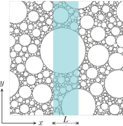
We discuss in some details the construction of the 2D L´evy glass; see Fig.1—the 3D version is entirely analogous. We start by generating disks of (dimensionless) radius
rk =rmax
1+ k kmax
rmaxβ −1 −1/β
,
FIG. 1. (Color online) Two-dimensional L´evy glass, consisting of a random packing of disks with a power-law distribution of radii (α=0.7,f =0.86, andrmax/rmin=100). The blue shaded region defines a slab of thicknessL. This is the unconstrained geometry, because the maximum disk size can be larger thanL.
Thekmax+1 disks have radii ranging fromrmin≡1 tormax 1, and in this size range their distribution follows the power law (2.1). The average area of a disk is
A = πβ |2−β|max
1,rmax2−β. (2.4)
The entire L´evy glass occupies an area of dimensionW ×W in the x-y plane, with periodic boundary conditions and W about 10–100 times larger thanrmax. For a random packing, we place the disks at randomly chosen positions in the order k=0,1,2, . . . (so starting from the largest disk). If disk number k overlaps with any of the disks already in place, another random position is attempted. For each disk, some 104 attempted placements are made. If they are all unsuccessful, the entire construction is started over with a smaller value of kmax.
The density of the packing is quantified by the filling fraction
f =kmaxA/W2. (2.5)
For each simulation, we strove for maximalf by maximizing kmax. The maximal filling fraction increases with increasing ratiormax/rmin, as illustrated in Fig.2. For the smallestα, below about 0.4, we could not reach as dense a packing as for larger α, basically because there are too few small disks. Somewhat larger filling fractions would be reachable by moving the disks after placement, but we did not attempt that.
B. Dynamics
The ballistic dynamics inside the spheres consists of chords of varying length s traversed in a time s/v. The diffusive dynamics in between the spheres is modeled by a Poisson process: isotropic scattering in a time intervaldt with probabilityv dt / lmfp. The mean free pathlmfp=rmin/2 is chosen such that there is, on average, one scattering event between leaving and entering a sphere. We take the same refractive index (and velocityv) inside and outside the spheres, so the ray is not refracted at the interface.
FIG. 2. (Color online) Filling fraction of the 2D L´evy glass as a function of the ratiormax/rminof largest and smallest disk size, for several values of the parameterα.
In Fig.3, we show the step size distributionp(s) for a 2D L´evy glass with disk radius distribution (2.1), forβ =2.2. It follows closely the L´evy distribution (2.2), with the expected parameter valueα=β−1=1.2 (solid line).
We do not find the pronounced oscillations inp(s), which in Ref. [10] complicated the determination of α. These oscillations appear due to coarse graining of the disk size distributionn(r) and vanish if a finer distribution of disk sizes is used.
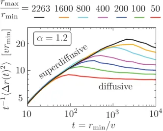
The time dependence of the mean-squared displacement r(t)2is shown in Fig.4, for the sameα=1.2. A particle was started at a random position r(0) in the interdisk region, and then its position r(t) at time t (either inside or outside a disk) gives the displacement r(t)= |r(t)−r(0)|. The average · · · is over some 104 initial positions. In accord with previous simulations [4,10], regular (Brownian) diffusion with r(t)2 ∝t is reached for timest r
max/v≡tD, set by the time needed to traverse the largest disk. For t < tD,
FIG. 4. (Color online) Time dependence of the mean-square displacement (divided by t so that saturation indicates diffusive scaling). The curves are the results of a numerical simulation in a 2D L´evy glass with different values ofrmax/rmin, at fixedα=1.2. The ratiormax/rmindecreases from top to bottom.
the mean-squared displacement increases more rapidly than linearly (superdiffusion).
The limiting slope of the mean-square displacement for ttD gives the diffusion constant in the Brownian regime,
D= lim t→∞
1
2dtr(t)
2. (2.6)
As shown in Fig.5, this diffusion constant has a power-law dependence onrmax,
D(rmax)∝r1−γD
max , (2.7)
with 0< γD<1. (For the smallestα=0.2, no clear power-law scaling was observed.)
FIG. 5. (Color online) Diffusion coefficient (2.6) in the Brownian regime, estimated from the large-tslope of the mean-square displace-ment (corresponding to the large-tsaturation value in Fig.4). Each set of colored data points represents one value ofα, with different values ofrmax/rmin. The power-law scaling (2.7) (red dotted lines) determines the scaling exponentγD.
D. Unconstrained geometry
A lower limitTballto the transmission probabilityTunconin the unconstrained geometry follows by considering only bal-listic rays, which pass through the region 0< x < Lwithout a single scattering event. As explained in the Appendix, see Eq. (A7), this probability is directly related to the step size distribution,
Tball= 1 s
∞
L dx
∞
x
ds p(s). (2.8)
We take the step size distribution (2.2) with an upper cutoff at smaxrmaxLand a lower cutoff atsmin1. Then Eq. (2.8) evaluates to
Tball
rmax−α−1L1−αrmaxα rmax−rmaxα
→rmaxL
1 for 0< α <1,
L1−α for 1< α <2. (2.9)
Since TballTuncon1, we can immediately conclude thatTuncon=1 for 0< α <1. For 1< α <2, the power-law scaling Tuncon∝1/Lγ must satisfy γ α−1. This holds irrespective of correlations between multiple steps, since these cannot affectTball. If we neglect these correlations, we may equate Tuncon to the transmission probability Teq of a L´evy walk with equilibrium initial conditions (see AppendixA3). In view of Eq. (A9), this leads toγ =α−1. We believe this result to be quite robust, since even if correlations do play a role, it is likely that they slow down the superdiffusion [7,8], so they would not lead to a smallerγ.
In Fig.6, we show theLdependence ofTunconfor two values ofα, resulting from a numerical simulation of an unconstrained 2D L´evy glass. This is data up to rmax=104 for α=1.1 and up tormax=103forα=1.5, which is at the upper limit of our computational resources. As expected from the L´evy walk (Fig.13), the convergence to thermax→ ∞limit is very slow, and we are not able to conclusively test the predicted asymptote.
E. Constrained geometry
FIG. 6. (Color online) Transmission probabilityTunconthrough a 2DunconstrainedL´evy glass, for different values of the maximum disk radiusrmax. The dotted line is the predicted scalingTuncon∝L1−α
in thermax→ ∞limit.
step size smaxL/2. From the analysis in Appendix 4b we would therefore expect a T ∝1/Lα/2 scaling of the transmission probability—if correlations between step sizes would not matter.
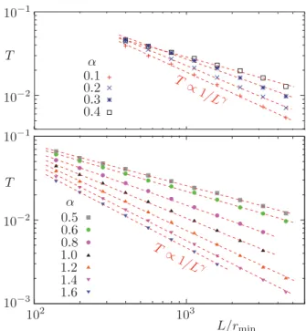
In Fig. 7, we show the scaling of the transmission probability,
T ∝1/Lγ, (2.10)
as it follows from the simulation. The power-law scaling applies to somewhat less than two decades inLforα0.5 (lower panel), and to one decade for smallerα(upper panel). In Fig. 8, we give the resulting exponent γ as a function ofα.
In the same figure, we show the scaling of the diffusion exponentγD, from Eq. (2.7). (There we could only obtain a power-law scaling for α0.4.) As expected from the identification of T D(L)/L∝1/LγD, one has in good approximation
γ =γD. (2.11)
III. COMPARISON WITH EXPERIMENTS
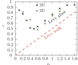
The numerical data shown so far was for a 2D L´evy glass of disks. We have also performed simulations for a 3D L´evy glass of spheres, in the constrained geometry withrmax=L/4. We went up toL/rmin=1132 forα0.8 and up toL/rmin=800 forα=1 and 1.2. (Larger values ofαcould not be simulated reliably.) Although the systems are smaller in 3D than in 2D, the results are quite similar; see the comparison in Fig.9 of theαdependence of the transmission exponentγfor a 2D and a 3D L´evy glass. In particular, for both 2D and 3D, the results forγlie well above theγ =α/2 line.
FIG. 7. (Color online) Transmission probability through a 2D constrained L´evy glass as a function of the thickness of the slab, for different values of the step size exponentα. The dotted lines are a linear fit to the data points, determining the transmission scaling exponentγ. (The data is split over two panels, to avoid overlap.)
We can now compare directly with the 3D experiments [4], which obtainedγ =0.5 within experimental accuracy for α=1. Our simulation, in contrast, gives forα=1 a value for γ that is about 50% higher. We cannot attribute the difference to finite-size effects, since the 3D simulation reaches the same range of system sizes as the experiment. There are aspects of the experiment that are not present in the simulation (notably absorption), but we believe that the difference is mainly due to an irregularity in the experimental sphere size distribution.
FIG. 8. (Color online) ExponentsγandγD, governing the scaling
FIG. 9. (Color online) Comparison of theαdependence of the transmission exponentγfor a 2D and 3D L´evy glass. Both data sets lie well above theγ =α/2 line of a L´evy walk.
To visualize the irregularity, we plot in Fig.10the quantity
V(r)= 4 3π
∞
r
r3n(r)dr, (3.1)
which is the cumulative volume enclosed by spheres with radii greater thanr. This is a decreasing function ofr, from V(rmin)=V0(the total sphere volume) down toV(rmax)=0. For the L´evy distribution withα=1 in 3D we haven(r)∝ r−4, cf. Eqs. (2.1) and (2.2); hence V(r) should decrease linearly as a function of logr,
V(r)= − V0 log(rmax/rmin)
log(r/rmax). (3.2)
As shown in Fig.10, the experimental sphere size distri-bution differs markedly from the expected L´evy form (3.2). Rather than a single linear dependence ofV(r) on logr, there are two piecewise linear dependencies with a different slope, joined with a kink at r≈50μm. This irregularity has the effect of reducing the transmission exponentγ, essentially by mimicking a system with a smaller value ofα.
To demonstrate the effect of the kink on the transmission exponent, we have simulated the experiment by constructing
(
)
FIG. 10. (Color online) Sphere volume distribution used in the experiment [4] (red solid histogram) and for an α=1 L´evy distribution (green dashed histogram).
with a divergent second moment of the step size distribution (α <2).
As a consistency check on our simulations, we have also calculated the diffusion constantDfrom the long-time limit of the mean square displacement in an unbounded L´evy glass, as a function of the maximum disk sizermax. We find D(rmax)∝r1−γD
max , with γD ≈γ, as expected for a diffusive transmission probabilityT D(L)/Lwith a scale-dependent diffusion constant.
Qualitatively, our finding that diffusive scaling of T can coexist with a divergent second moment ofp(s) is consistent with analytical calculations for d =1 [5] and d =2,3 [9]. Quantitatively, we are not in agreement: Ref. [9] finds that γ increases monotonically ford =2 fromγ =0 atα=0 to γ =1 forα1, while our simulation gives a nonmonotonic αdependence ofγ, with a saturation forα1.5 (see Fig.8). The system considered in Ref. [9] is quasiperiodic (a L´evy quasicrystal), rather than the random L´evy glass studied here. Further study is needed to see whether this difference is at the origin of the different transmission scaling, or whether the difference is due to a very slow convergence to the infinite system-size limit (which we consider more likely).
ACKNOWLEDGMENTS
This research was supported by the Dutch Science Founda-tion NWO/FOM.
APPENDIX: TRANSMISSION PROBABILITY OF A L ´EVY WALK
1. Formulation of the problem
We consider a random walk along thexaxis with the power-law step size distribution
p(s)= α s0
s0 s
1+α
θ(s−s0). (A1)
[The functionθ(s−s0) equals 1 if s > s0 and 0 if s < s0.] Subsequent steps are +s or −s with equal probability and independently distributed. The probability densityp(s) decays as 1/s1+αwithα >0, starting from a minimal step sizes
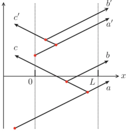
FIG. 11. (Color online) Trajectoriesx(t) of a random walk, with scattering events indicated by red dots. All trajectories enter the segment 0< x < L (between dotted lines) at x=0. Trajectories a,b,a,b are transmitted throughx=L, while trajectoriesc,c are reflected throughx=0. The transmission probabilityTeq averages over all trajectories (equilibrium initial conditions), while Tnoneq averages only over trajectories such asa,b,cthat have a scattering event upon entering the segment at x=0 (nonequilibrium initial conditions).
The walker enters the segment 0< x < L by passing throughx=0 at timeti and then stays in that segment until timetf. If attf it exits throughx =L, we say the walker has been transmitted through the segment. We seek the dependence of the transmission probability T on the length L of the segment, for Ll0. For a Brownian walk, the scaling is inverse linear:T ∝1/Lifα >2. For a L´evy walk, we expect a slower power-law decay,T ∝1/Lγ withγ <1. The question is howγ varies withα <2.
The answer depends on how the walker is started off initially. Following Barkai, Fleurov, and Klafter [12], we distinguish equilibrium from nonequilibrium initial condi-tions. (See Fig. 11.) For equilibrium initial conditions, the walker starts off from x= −∞, so that it crosses x =0 at some random time between two scattering events. For nonequilibrium initial conditions, the walker starts off from x=0 with a scattering event. We denote the transmission probabilities in these two cases byTeqandTnoneq, respectively, and consider the two cases in separate subsections.
2. Nonequilibrium initial conditions
The transmission probabilityTnoneq fromx =0 to x=L for a L´evy walk that starts off with a scattering event atx =0 has been calculated by several authors [13–15]. We give the most general solution of Buldyrevet al.[15].
They assume that the walker starts with a scattering event at an arbitrary pointxi in the segment (0,L) and calculate the probabilityP(xi) that the walker exits the segment through x=L. For Ls0 andxi s0, their solution [15] can be written in the compact form
P(xi)=
B(xi/L,α/2,α/2)
B(1,α/2,α/2) , (A2)
in terms of the incomplete beta function
B(x,a,b)=
x
0
ya−1(1−y)b−1dy. (A3)
SinceB(x,a,b)→xa/aforx →0, one arrives at the scaling Tnoneq∝L−α/2, first obtained by Davis and Marshak from basic considerations [13].
The prefactor of the power-law scaling cannot be obtained directly from the solution (A2), because of the limitation that xis0. For 0< α <1, we can work around this limitation by considering the first step separately. The walker starts off at x =0 with a step to x1>0, chosen randomly from the distribution (A1) of a L´evy walk. If x1> L, the walker is transmitted with unit probability. Otherwise, it is transmitted with probabilityP(x1).
We thus can calculateTnoneqfrom
Tnoneq=
∞
L
dx1p(x1)+
L
0
dx1p(x1)P(x1). (A4)
Forα <1, the mean step size diverges, so the regionx1s0 is insignificant and we can use Eq. (A2) forP(x1). The result is
Tnoneq =
B(s0/L,α/2,1+α/2) B(1,α/2,1+α/2)
Ls0
→ s0 L α/2 4(α)
α2(α/2). (A5)
While the exponentα/2 holds for any 0< α <2, the prefactor is accurate only for 0< α <1. [Forα >1, we would need to knowP(x1) within the regionx1s0in order to calculate the prefactor.]
3. Equilibrium initial conditions
For equilibrium initial conditions, the walker crossesx =0 at a random time between scattering events. The first subse-quent scattering event is at a point x1 >0, with probability densityq(x1). Ifx1> L, the walker is transmitted with unit probability; if 0< x1< L, the transmission probability is P(x1). Hence
Teq=
∞
L
dx1q(x1)+
L
0
dx1q(x1)P(x1). (A6)
The probability densityq(x) is determined from the step size distribution,
q(x)= 1 s
∞
x
p(s)ds. (A7)
This relation between the distribution p(s) of the distances between subsequent scattering events and the distributionq(x) of the distancexfrom an arbitrary point to the next scattering event holds for any random walk with a finite average step size s =0∞sp(s)ds. For the step size distribution (A1), one has
q(x)= α−1 αs0
s0 max(x,s0)
α
, for α >1. (A8)
The value α=2 at the border between a Brownian walk and a L´evy walk requires separate consideration. While Tnoneq∝1/Lforα=2, the transmission probability (A6) has a logarithmic enhancement,
Teq= s0 L
1+1 2ln
L
s0 , for α=2. (A11)
A similar but different scaling∝L−1√lnLhas been associated with theα=2 L´evy walk in Ref. [14].
4. Truncated L´evy walk
AtruncatedL´evy walk has step size distribution
ptrunc(s)= α s0
s0 s
1+α
θ(s−s0)θ(smax−s), (A12)
with a maximum step sizesmaxs0. The root-mean-squared displacementσ after a single step then has a finite value,
σ =
α 2−αs
1−α/2 max s
α/2
0 , (A13)
much smaller thansmaxforα <2.
The transition from a truncated L´evy walk to a Brownian walk requiresnsteps1 of steps, given by Refs. [16,17]
nsteps
(2−α)3
α (smax/s0) α.
(A14)
The corresponding root-mean-squared displacement σ√nsteps(2−α)smax is of order smax for all α <2. We conclude that we have regular (Brownian) diffusion over a distanceLifsmaxL.
The transmission probability P(x) for a walker starting with a scattering event at a pointxinside a slab of thicknessL (further thansmaxfrom the boundaries) thus follows the usual diffusive scaling,
P(x)=x/L, if x,L−xsmax. (A15)
a. Equilibrium initial conditions
For equilibrium initial conditions, the distribution q(x) of the first scattering event follows from Eq. (A7), with p
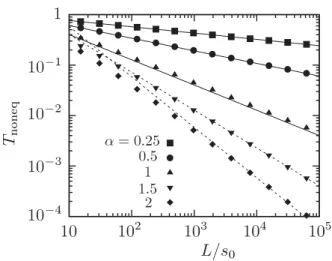
FIG. 12. Transmission probabilityTnoneqof a L´evy walk through a slab of thicknessL, fornonequilibriuminitial conditions. The data points are the results of a numerical simulation, for different values of the step size exponentα(and fixedsmaxL). The lines indicate the expectedL−α/2 scaling. Forα <1, we also have an analytical prediction (A5) for the prefactor (solid lines), while forα >1 only the exponent is known analytically so the prefactor has been fitted to the data (dotted lines).
replaced byptrunc. Substitution into Eq. (A6) then determines the transmission probability (forL > smax),
Teq=
smax
0
dx q(x)P(x). (A16)
Equation (A15) givesP(x) only forx smax. We will use this expression also forx < smax, and then test the approximation by comparing with numerical simulations in Sec. V.
If we substituteP(x)=x/L, we find
Teq= 1 2L
1−α 2−α
smax2 −smaxα s02−α smax−sα
maxs1− α 0
, (A17)
for 0< α <1 or 1< α <2. Forα=1 or α=2, there are logarithmic factors,
Teq =
smax−s0 2Lln(smax/s0)
, for α=1, (A18a)
Teq = s0 2L
smaxln(smax/s0)
smax−s0 , for α=2. (A18b)
For fixedsmax, the diffusive 1/Lscaling holds. An anomalous scaling appears if the maximum step sizesmax=cLis a fixed fraction c <1 of the slab thickness. Then the transmission probability through the slab depends onLs0as
Teq= 1 2c
2−α
s0 L
α−1α− 1
2−α, for 1< α <2, (A19a)
Teq= 1 2c
1−α
2−α, for α <1, (A19b)
Teq= c 2 ln(cL/s0)
, for α=1, (A19c)
Teq=
s0ln(cL/s0)
FIG. 13. (Color online) Transmission probabilityTeq of a L´evy walk through a slab of thicknessL, forequilibriuminitial conditions. The two panels are for different values of α. The data points result from a numerical simulation, with different values smax of the maximum step size. The solid line is the asymptote (A9) for smax→ ∞.
HenceTeq∝1/Lmax(0,α−1) (with logarithmic corrections for α=1 andα=2). This is the same scaling as for the L´evy walk without truncation (see Sec.III).
b. Nonequilibrium initial conditions
For nonequilibrium initial conditions, the transition to the regular diffusive regime happens while the walker is inside the slab. We may therefore assume that the usual diffusive scaling Tnoneqσ/Lapplies (withσplaying the role of the mean free path). In view of Eq. (A13), an anomalous scaling appears if smax=cLscales proportionally toL,
Tnoneq(cL)1−α/2s α/2
0 L−1 ∝L−
α/2. (A20)
The anomalousL−α/2 scaling of AppendixA2 now appears as a consequence of regular diffusion with a scale-dependent mean free path.
5. Numerical test
We have tested the analytical expressions (A5) and (A9) by numerical simulation. Results forTnoneqare shown in Fig.12. This is the nonequilibrium initial condition, where the walker starts off atx=0 with a step to positivex. TheL−α/2scaling is reproduced for all 0< α <2, and the prefactor (A5) agrees well with the simulations for 0< α1.
For the equilibrium initial condition, the walker starts off at a large distance fromx =0, crossing the boundary at a random
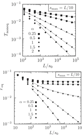
FIG. 14. Transmission probability for a L´evy walk with maxi-mum step sizesmaxthat increases proportionally toL. The two panels (both forsmax=L/10) correspond to equilibrium and nonequilibrium initial conditions. The dotted lines show the expected scaling (A19) and (A20), up to a prefactor that has been fitted to the data. [ForTeq the difference with Eq. (A19) is a factor of 2, independent ofα.] point between two scattering events. Results of numerical simulations are shown in Fig.13. Unlike in the nonequilibrium case, the convergence to the asymptotic scaling with increasing smaxis very slow, in particular for smallα.
We have also tested the scaling (A19) and (A20) for a truncated L´evy walk with a maximum step size smax that is a fixed fraction of L. Results are shown in Fig. 14 for both equilibrium and nonequilibrium initial conditions. The anomalous scaling now appears, even though the diffusion is regular on the scale of L, because of the scale dependence of the mean free path. For both types of initial conditions the numerics follows closely the analytically predicted power laws, including the logarithmic factors for α=1,2 in the equilibrium case. (The constant prefactors are not given reliably by the analytics.)
[1]L´evy Flights and Related Topics in Physics, edited by M. Shlesinger, G. Zaslavsky, and U. Frisch (Springer, Berlin, 1995).
[2] R. Metzler and J. Klafter, Phys. Rep. 339, 1 (2000).
[11] References [4,10] use a different relation β=α+d−2 be-tween the exponents in Eqs. (2.1) and (2.2), because their
en-(1994).