Stochastic Decision Making in Manufacturing Environments

(1)

Stochastic Decision Making in Manufacturing Environments

Abdollah Arasteh

∗

Assistant Professor, Industrial Engineering Department, Babol Noshirvani University of Technology, Babol, Iran

Abstract

Decision making plays an important role in economics, psychology, philosophy, mathematics, statistics and many other fields. In each field, decision making consists of identifying the values, uncertainties and other issues that define the decision. In any field, the nature of the decisions is affected by environmental characteristics. In this paper, we are considered the production planning problem in a stochastic and complex environment, i.e. the environment of electronic equipment production, where planning is faced with variable results and changeable requests. In this complicated environment, we are encountered with joint replenishment, variable yields and exchanging demands and many other complex variables related to inventory management and control systems that have complicated and unpredictable behavior and could not be modeled in a simple way. We are trying to model this environment as a stochastic problem. The aim of mathematical model is managing and controlling inventories in such a complex production environment. We also try to solve the proposed stochastic problem by estimation procedures. The planning problem is devised as a gain-maximizing stochastic program. Also we use two mathematical and simulation software to predict the behavior of production system in various situations. The results of simulations are mentioned in the paper.

Keywords: Manufacturing, Decision making, Inventory policies, Stochastic yield

1- Introduction

In every collecting environment the yield’s way is managed by paying little heed to whether the thing meets the client’s necessities. In a couple cases, a harmed respectable can be repaired and in diverse cases it might must be hurled. There are various circumstances where a thing which not meets its determination, may be fitting for some other use. For instance, in the electronic business, the capacitors and resistors are suitable examples. The utilization that an electronic connector finds is to some degree managed by the precision of its strings and the metal's exactness plating. This is genuinely fundamental in the electronic and particularly in the semi-conductor industry. Electronic gear generation frameworks and distinctive circumstances that incorporate impelled advances, things and creation developments are rapidly being used to make novel things and headways. Therefore, the creation increments can be outstandingly unsteady (Crevier, Cordeau et al. 2007, Lin and Huang 2014, Ashayeri, Ma et al. 2015, Lin and Chen 2015).

In this paper, we consider conditions in which the product categories can be ranked. We suppose that a product in a higher category can be replaced by a product that is lower in the hierarchy. Under these conditions, the manufacturer may sometimes downgrade the category of a product rather than backorder a lower-grade item. This kind of activity may be persuaded by some reasons, for case - to avoid client

*Corresponding author.

Journal of Industrial and Systems Engineering

Vol. 9, No. 1, pp 17-34

Winter (January) 2016

17

(2)

disappointment; to decrease set-up expenses; or to reduce inventory costs. We are occupied with recognizing suitable demand arrangements in a domain of stochastic yields and substitutable demands. Our enthusiasm for this issue came about because of a particular application in the semi-conductor industry. For the purpose of solidness we will portray this application in more noteworthy subtle element. The case discussed in this paper is especially relevant to the semi-conductor industry. In the semi-conductor industry, items and assembly technologies change quickly. The assembling procedure is mind boggling and regularly not exceptionally surely knew. Therefore yields change essentially. Choice guides that encourage stock administration in this questionable environment can be assumed as an essential part in enhancing productivity (Ponsignon and Mönch 2014, Zhang, Qin et al. 2014, Rotondo, Young et al. 2015).

A number of electronic components, such as semi-conductor chips, are produced from wafers. Each wafer may produce thousands of chips. The chips produced in such a facility using the same wafer often show different electrical properties. In other words, the requests are changeable. In addition, the mixture of chips produced from the wafer differs from one lot to the next. As a consequence, in this system, the results and requests are changeable because the chips are cooperatively restored (Yao, Jiang et al. 2011). In this paper, we consider a mathematical model to help managers to decide (a) how many wafers to produce each time and (b) how to assign chip inventories to the end users. The problem is formulated as a stochastic program. The size of the model grows rapidly; therefore, approximation algorithms are used to solve the stochastic program.

The wafer production facility is shared by many product families. This facility includes many costly machines, and several product families share these resources. Consequently, production batch queues are in front of these machines. The three elements that production managers monitor to control the proper capacity levels are trade-offs between work-in-process (WIP) costs, lead times and the cost of extra capacity (Adacher and Cassandras, 2014 and Hosoda, Disney et al. 2015). Supporting this decision requires theoretical models that can provide insight into the long-term behavior of the facility. Queuing network models of the wafer production facility are practical in this respect (Bitran and Tirupati 1988). In almost every manufacturing environment, the nature of the yield is dictated by how well the item coordinates the needs of the client. In a few cases, a blemished decent can be repaired; in different cases, it may not be useable. Much of the time, an item that does not meet the necessities of an application may be suitable for some other utilization. For instance, the nature of capacitors and resistors in the hardware business is controlled by their resistances (Sethi, Taksar et al. 1995).

In this paper, we consider conditions in which the output categories are ranked. We suppose that a product in a higher category can be replaced by a product in lower stage of the hierarchy. Under these conditions, the manufacturer may sometimes downgrade the category of a product rather than backorder a lower-grade item. We are trying to determine proper inventory and control policy in an environment of stochastic variables. Our aim in this problem arose from a case study in a real world semi conductor production environment. However, a broad range of inventory management and control problem nearly have equivalent characteristics.

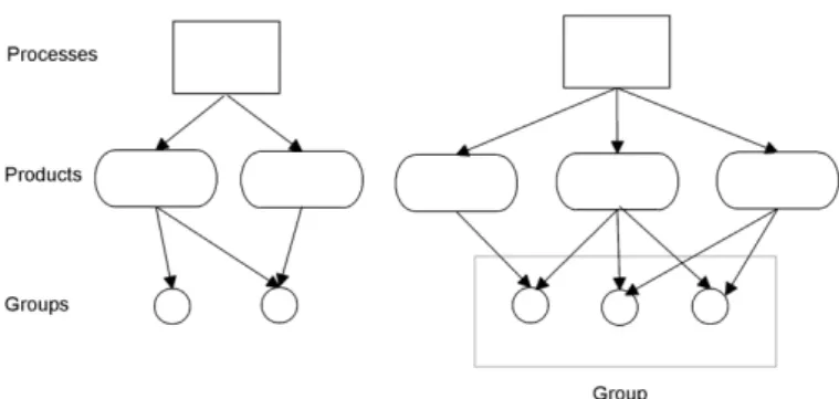
In electronic industry, technologies can change quickly. The manufacturing processes are complex and frequently not well understood. As a result, the manufacturing yields can differ greatly. Decisions that support simple inventory management in an unknown condition can significantly increase profitability (Flapper, Gayon et al. 2014, Sarkar, Mandal et al. 2015). In this paper, we examine (i) the processes, (ii) the elements and (iii) the applications of these decisions for customers. “Process” refers to the production process for a wafer, and “element” refers to diode.Relevant to each process is a set of elements that can be produced using that process. The real yields are random variables. The distributions of these random variables are controlled by the production process that is being performed (Jane and Laih 2005). This type of action may be prompted by a variety of causes, such as eliminating customer dissatisfaction, decreasing setup costs, and decreasing inventory costs (Feng, Wua et al. 2010). We suppose that customers can be divided into groups. Within each group there is a ranking such that a product that is proper for an element in the group is also proper for all elements lower in the ranking. The relation between processes, products and groups is shown in figure 1.

(3)

Figure 1. Relations between processes, products and groups

Our objective is to propose a model that helps managers to determine how many elements to produce by each process. Once the products are known, the model will help the managers determine how to assign the elements to the customers. One goal of this work is to improve the management of element inventories. We devised the problem as a benefit-maximizing convex stochastic program and developed evolved approximation algorithms to solve the program. Based on a two-time problem structure, we suggest heuristics for assigning the elements to the customers in a multi-period setting.

2- Literature Review

There is a vast body of literature related to inventory and production planning. In most of the inventory models, the yield is assumed to be 100% or is assumed to be definite and known. Few papers address yield variability. Vienott analyzed the early literature on essential lot-sizing models (Veinott, 1960). Silver obtained the economic order quantity (EOQ) when the quantity from the supplier matched the quantity ordered. He allowed the probability density of the quantity obtained to be a function of the quantity ordered (Silver, 1976). Kalro and Gohil expanded Silver’s model to the case where the request during the stock-out period is either relatively or completely backordered (Karlo and Gohil 1982). Shih considered a single-period model with random requests, variable yield and no ordering costs (Shih 1980).

Mazzola, McCoy, and Wagner analyzed a multi-period problem using an EOQ model in which the production yield followed a binomial distribution and the request could be backlogged. They tested several heuristics to separate the time problems (Mazzolla, McCoy et al. 1987).

The heuristics with the most potential were used to adapt the definite lot-sizing policies, which were optimally computed using the Wagner-Whitin or the Silver-Meal heuristic. Some researchers have demonstrated a multi-stage single period single item issue. They accepted that the extent of inadequate pieces delivered at every stage is an arbitrary variable. The choice variables are the amounts to be created at every stage. These choices are to be made after you know the quantity of good pieces delivered by the past stage. At every stage you bring about generation and holding expenses. Unsatisfied interest results in punishments as backorder expenses. They demonstrate that the expense acquired at every stage is a curved capacity of the amount delivered at that stage and other useful results (Lee 2014, Lee, Oh et al. 2014, Melouk, Fontem et al. 2014, Sprenger and Mönch 2014, Yeh, Realff et al. 2014).

Another interesting problem in this area that has been considered by some researchers is by-product problem that has been contemplated by Pierskalla and Deuermeyer for the first time (Deuermeyer and Pierskalla, 1978). In this problem, we consider the control of a generation framework that comprises of two procedures that produce two items. Process A produces both items in some altered (deterministic) extent while process B creates one and only one item. We expect that the demands are arbitrary. Researchers detail the issue as an arched program and determine a few properties of the ideal approach and demonstrate that the choice space (stock levels) can be separated into 4 districts relying upon regardless of whether a generation procedure is utilized (Tan, Lee et al. 2014, Chung and Heshmati 2015, Samsatli, Samsatli et al. 2015). There is a considerable literature on computational techniques for settling stochastic programs (Chew, Lee et al. 2014, Elbanhawi and Simic 2014, Adulyasak, Cordeau et al. 2015, Capaldo and Giannoccaro 2015, Fagerholt, Gausel et al. 2015, Li and Womer 2015, Mohammadi, Musa et al. 2015, Zhang, Zheng et al. 2015). Dantzig performed one of the earliest investigations in this field (Dantzig 1955). Olsen demonstrated that the demand of arrangements of discrete rough guesses fulfills the arrangement of the ceaseless issue under genuinely slight conditions (Olsen, 1976). Birge and Wets adequately examined that the close estimation gets ready for a few stochastic advancement issues (Birge and Wets, 1986).

(4)

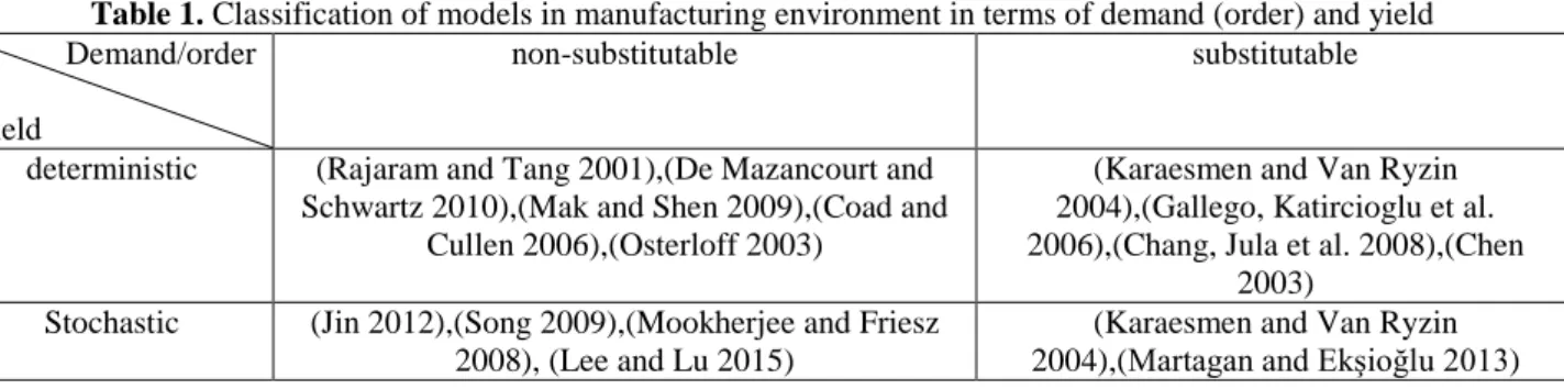
Thus far, there have been few published models of production processes in which the demands are changeable and have stochastic results. In a sense, our model generalizes the idea of a “fault” by allowing a number of quality classes. Although the analysis is limited to a special change form, this form is likely the most ordinary change form. First, we express the general model in which the demands and lead times are probabilistic; then, we explain the modeling assumptions and the formulation (Fujimoto and Park 2014, Dasgupta and Roy 2015, Shin, Park et al. 2015). Table 1 shows a proposed classification of various models in this research area.

Table 1. Classification of models in manufacturing environment in terms of demand (order) and yield Demand/order

Yield

non-substitutable substitutable

deterministic (Rajaram and Tang 2001),(De Mazancourt and Schwartz 2010),(Mak and Shen 2009),(Coad and

Cullen 2006),(Osterloff 2003)

(Karaesmen and Van Ryzin 2004),(Gallego, Katircioglu et al. 2006),(Chang, Jula et al. 2008),(Chen

2003) Stochastic (Jin 2012),(Song 2009),(Mookherjee and Friesz

2008), (Lee and Lu 2015)

(Karaesmen and Van Ryzin 2004),(Martagan and Ekşioğlu 2013) To the best of our knowledge, there are very few papers demonstrating a creation process where the demands are substitutable and the yields are stochastic. One might say our model sums up the idea of “deformity” by allowing various evaluations of value. We do limit the investigation to a specific substitution structure. On the other hand, this structure is likely to be the most characteristic and basic substitution structure.

3- Modeling assumptions and problem formulation

To expand the mathematical model, we had to make a few key assumptions regarding the demand designs and the varying nature of the processes. The customers for the diodes are manufacturers of electronic goods who identify their needs over a period of approximately 6 months. The carriage schedule identifies the quantity to be sent each week. Accordingly, we suppose that the demands are dynamic and definite. As previously stated, several models of inventory control are available. In some models, deterministic demands (or demands with small alternate possibilities that can be discarded) are used (Polyakovskiy and M'Hallah 2014, Varas, Maturana et al. 2014, Zhang and Wang 2014). Nonetheless, there are models with more sensible suspicions that consider probabilistic solicitations. In this paper, we concentrate on the first class of models and its suppositions (Safaei and Thoben 2014, Eğilmez and Süer 2015, Zhu, Li et al. 2015). In any case, we dole out a segment of the paper for the second class of models.

In the first category, a minimum of two models, the additive and the multiplicative, are used to vary the output. In the additive model, the number of type k items obtained from producing n units isno_k +

ε

_k, where

k

o is a constant that depends on the operation, and

ε

_k is an arbitrary variable. In the multiplicative model, the output is directly given byno_k, where o_k is an arbitrary variable. The sum of the two o_k values must be less than or equal to one. We modify the multiplicative model and assume a limited number of outcomes. The objective of our model is to maximize the expected gains. Customers higher in the hierarchy pay a higher price. The costs include the production cost, holding cost and backorder cost. We assume that there are no setup costs. We now formulate the problem based on the above assumptions. We first describe the model for deterministic demand. To simplify the presentation, we first consider a single-period problem with zero lead time and disregard capacity limitations. We then expand our consideration to family, multi-period problems and describe how to include capacity limitations.

Because we begin with unlimited capacity, the problem can be distinguished by families. In this section, we consider the single-family problem. Moreover, we define the problem by assuming that there are only two customers in the family. The members of the family are numbered in descending order (i.e., the highest member of the family is denoted by 1). We also number the items. An item can only be assigned to a family member with a number that is appropriate for the item’s number. Thus, item #1 can be used for customer 1 or 2, whereas item #2 can be used only for customer 2.

We suppose that production begins at the start of the day and ends in the evening; therefore, the products are known. In the evening, the items are assigned to the customers. The general goal of our problem is to

(5)

maximize profit. We suppose that customer 1 pays a higher price than customer 2. All of the excess inventories can be sold at a rescue price. Backorder, inventory holding and production costs are incurred without any setup costs. In this structure, the number of units to produce in the morning must be decided, and the item assignment in the evening must be optimized. The following variables are used:

ij

N : the number of i items assigned to customer j (because item 2 cannot be assigned to customer 1, we do not obtain

A

₂₁);

ti

π

: the backorders for customer i, moved into period t; i

R : the rescue price for item i; ti

D : the request from customer i in period t; o

S : the supposition concerning the outputs; ti

I : the inventory of item i, moved into period t; C : the production cost per unit;

M : the number of units produced;

) ( a a v

u : the sector of the item with the ath issue of the arbitrary variables; i

P: the price paid by customer i; and i

θ

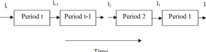
: the backorder cost for customer i.

The periods are indexed in reverse order. The index specifies the number of periods remaining in the planning horizon. In this notation, period 1 is the last period in the planning horizon, and period 2 is the next to the last period. The scheme of this sequence is illustrated in figure 2.

Figure 2. The time indexing

The morning problem consists of

0

) 1 , 1 , , ( 1 max

) 1 , 1 ( 1

≥

− =

m st

Cm I

m a u G o S I

f π π

(15)

The evening problem consists of

11 1

, 0 12 11 :

2 1 0 2

1 0,1 )

22 12 ( 2 11 1 max ) 1 , 1 , , ( 1

I a mu I

N N st

i i i i RiI

N N P N P I

m a u G

+ = + +

∑ = − ∑

= + + +

= θπ

π

(16)

N₂₂ +I₀₂ =mv_a+I₁₂ Balance (17)

11 11 01

11+π = D +π

N Demand constraints (18)

(6)

N₁₂+N₂₂+π₀₂ =D₁₂ +π₁₂ (19)

N₁₁,N₁₂,N₂₂,π₀₁,π₀₂,I₀₁,I₀₂ ≥0 (20)

Constraints (2) and (3) represents the inventory balance. The right-hand side of the equation represents the inventory of each element that is obtainable by the end of the day (because the production and the yields are known in the evening). Constraints (4) and (5) represent the customers’ demands. The right-hand side of the equation is the net demand, and the left-hand side illustrates how the demand is fulfilled.

3-1- Convexity

We first illustrate that the one-period problem is convex.

Hypothesis 1: for any outcome, u_aG(u_a,.) is a concave function of

A

,

I

₁

,

π

₁ and D1. Hypothesis 2: the morning problem is convex.

Hypothesis 3:

f

₁

(

I

₁

,

π

₁

)

is concave.

These hypotheses are rational if the demand is not definite. The demand change framework can also be highly repetitive, allowing us to force capacity constraints. However, the framework would be demolished if the setup costs are significant and must be included. The hypotheses can also be expanded to a multi-period problem.

4 - Item Assignment Process

In a single-period problem, the assignment process is simple. To simplify the description, suppose that the starting inventories and backorders are zero. Let P₁+θ₁≥P₂+θ₂ and R₁≥ R₂. The first inequality assures that the cost of preceding a selling to customer 1 is greater than that of customer 2. The second inequality requires that the rescue price of item 1 is higher than that of item 2. We also requireP_i +θ_i ≥R_i. As a result, it is suboptimal to backorder the demand for customer i and hold inventories of item i. Under these conditions, item j is first assigned to customer i. If these products are sufficient to match the requests, item 1 does not need to be assigned to customer 2; consequently, the entire surplus inventory will be utilized. The only conditions under which item 1 is assigned to customer 2 occur when the inventory of item 1 exceeds the request of customer l and the inventory of item 2 is less than the request of customer 2. In this condition, it will be optimal to lower the price of item 1 if the rescue price

R

₁ is less than

P

₂

+

θ

₂. Otherwise, it is optimal to obtain the inventories of item 1 and backorder the amount requested by customer 2. Hereafter, we will suppose that it is optimal to downgrade.

Next, we analyze the assignment process in a two-period problem. Suppose that the yields of the next to the last period are known and that assignment decisions must be made. In our model, the costs and the sale prices remain constant from period to period. Consequently, there will not be any backorder from customer j, and inventories of item j will be held. Again, the only interesting case is when there is a surplus of item 1 and a scarcity of item 2. In a single-period problem, we downgrade (if it is optimal to do so) until either the request of customer 2 is entirely satisfied or until we run out of item 1. Typically, this situation does not occur in a two-period problem. Only some of the surplus may be downgraded, and the final period may begin with an inventory of item 1 and by backordering the request of customer 2 (Barattieri 2014, Chang, Xia et al. 2015).

4-1- The structure of

f

₁

(

I

,

π

)

In this subsection, we make the following assumptions.

(1) I₁_j*

π

₁_j =0 for j = 1, 2. This assumption characterizes situations in which it is not optimal to backorder the demand of customer j and move item j into inventory in the next to the last period.

(2) I₁_j ≤D₁_j for j = 1, 2. Considering the other cases are neither interesting nor practical.

22

(7)

We make also a small adjustment in the notation by including the demands from the final periods in the topics of function

f

₁

(.,.)

. The definition of the function remains the same in all other respects.

We first illustrate how to transform the problem with initial inventories and backorders to one without initial inventories or backorders. Next, we test

f

₁

(

D

₁₁

,

D

₁₂

,

0 ,

0 )

over the area D₁_,₁≥0 to double, which illustrates that in the

(

D

₁₁

,

D

₁₂

)

space

f

₁

(

D

₁₁

,

D

₁₂

,

0 ,

0 )

is linear along any initially spreading beam.

Hypothesis 4:

If I₁_j ≤D₁_j for j=1, 2 then

) 0 , 0 , 12 12 12 , 11 11 11 ( 1 12 2 11 1 ) 12 , 11 , 12 , 11 , 12 , 11 ( 1 π π π π + − + − + + = I D I D f I P I P I I D D f (21)

Therefore, we can reformulate the evening problem as follows:

a mu I N N T S

i i i

i RiI I N N P I N P I D m a u G = + + ∑ = − ∑ = + + + + + = 01 12 * 11 . . 2 1 0 2 1 01 ) 12 * 22 12 ( 2 ) 11 * 11 ( 1 max ) 1 , 1 , 12 , , ( 1 π θ π (22) * 11 01 * 11 02 * 22 D N a mv I N = + = + π (23) * 12 02 * 22

12 N D

N + +π = (24)

0 02 , 01 , 02 , 01 , * 22 , 12 , *

11 N N I I ≥

N π π

(25) Thus, ) 0 , 0 , * 12 , * 11 , , ( 1 12 2 11 1 ) 1 , 1 , 12 , 11 , , (

1ua m D D I PI P I G ua m D D

G π = + + (26)

As a result,

) 0 , 0 , 12 12 12 , 11 11 11 ( 1 12 2 11 1 ) 12 , 11 , 12 , 11 , 12 , 11 ( 1 π π π π + − + − + + = I D I D f I P I P I I D D f (27)

23

(8)

In the next hypothesis, we illustrate that duplicating the demands is the optimal solution to duplication problem in the single-period problem with zero inventories and backorders.

Hypothesis 5: ) 0 , 0 , 12 , 11 ( 1 ) 0 , 0 , 12 , 11 ( 1 ,

0 then f D D f D D

Let ω≥ ω ω =ω

Hypothesis 6:

There exists an ordering, 0≤α₁ ≤α₂ ≤α₃ ≤...≤α_n ≤∞, such that α_i ≤D₁₁/D₁_,₂ ≤α_i₊₁,f₁(D₁₁,D₁₂,0,0) is linear.

4-2- Item Assignment in the Penultimate Period

Recall that after assigning item 1 to customer 1 and item 2 to customer 2, we will have

σ

units of item 1 and ∆ units of unsatisfied requests from customer 2. We have shown that assigning a unit of item 1 to customer 2 increases the penultimate period gains by

P

₂

+

θ

₂

+

d

₁ and changes the final period gains from

) , 0 , 0 , , 12 , 11 (

1 D D σ ∆

f to f₁(D₁₁,D₁₂,σ −1,0,0,∆−1). If the net change is designated

Γ

, then ) 1 , 0 , 0 , 1 , 12 , 11 ( 1 ) , 0 , 0 , , 12 , 11 ( 1 1 2

2+ + + ∆ − − ∆−

=

Γ P θ d f D D σ f D D σ .

Based on hypothesis 4,

) 0 , 0 , 1 12 , 1 11 ( 1 ) 0 , 0 , 12 , 11 ( 1 1 1 2

2+ + − + − −∆ − − + +∆−

=

Γ P θ d P f D σ D f D σ D .

Let D₁₁* , and D₁₂* be the net final period demands, i.e., D₁₁* = D₁₁−σ +ψ and D₁₂* =D₁₂+σ −ψ are the quantities of item 1 that are demoted. By demoting item 1 the ratio of D₁₁* /D₁₂* increases. Specifically, it is optimal to demote item 1 if

Γ

>

0

. The value of

Γ

will change whenever the demoting process moves us from one linear area of the function f₁(D₁₁* ,D₁₂* ,0,0) to the next. According to hypothesis 6, this process

occurs every time D₁₁* /D₁₂* becomes larger than

α

_i for some value of i. The demoting ends when

Γ

becomes negative, which leads to the following result (hypothesis 7).

There exists a non-negative number

α

* (perhaps=∞) such that it is optimal to proceed with demotion if and only if the following states are fulfilled:

. 0 ) 3 ( ; 0 ) 2 ( ; * * 12 / * 11 ) 1 ( ≥ − ∆ ≥ − < ψ ψ σ α and D D

In our problem, the combination of the output is arbitrary. Theoretically, we do not know the part of each item that will be used in the final product. We only know the probability of having a special part, which is independent from the production rate. Therefore, the optimal solution in a single-period problem could be to double the demands. Given the uncertainty of the results, hypothesis 7 is also intuitively attractive. Demoting changes parts of the net request and increases the proportion of item 1 that is necessary in the final period. Consequently, it is rational to cease demoting if the parts of item 1 that are required increase after some critical value

α

*. Although the essence of the optimal demoting strategy is instinctive,

α

* is hard to control because it relies on the cost parameters and the resulting distribution. Nevertheless, hypothesis 7 is intuitive and is the basis for the solution procedures that we suggest (Narayanan and Robinson 2010).

The nature of the optimal demoting strategy for a two-product, two-period problem is defined. The results can be expanded to a multi-product problem. Unfortunately, this procedure is not always optimal if the number of periods is greater than 2. In this case, the results expand to a multi-period problem only with definite yields. With stochastic yields, the demoting process is complicated and cannot be easily distinguished. Considering the difficulty of identifying the optimal demoting policy for multiple periods, we suggest using heuristics in finite-horizon problems. The rules are derived using hypothesis 7. We recommend the accompanying heuristics:

(9)

1) If 1 *_,

0

* , 1 / *

,

1 nn i

i

j∑ D n j D n i ≤ + −

= τ− + τ− + α in period

τ

, then assign item n to customer n+1, where *

, 1 j D_τ₋ is the practical or net request in period τ−1, i.e., D_τ*₋₁_,_j considers the backorders and inventories.

α

* is

determined such that i _n_n a

j un j un

P ∑− ≤ ₊ ≤

= + + )

* 1 , 1

0 / 1

( α .

2) This heuristic is essentially identical to heuristic (1). However, let α*=u′/v′, where u′ and v′ are the average results. Additionally, safety stocks are obtained.

5- Computational Procedures

In this section, we investigate the procedures for calculating the quantities to bemanufactured. We begin with unconstrained, single-family problems and then consider problems with capacity constraints. As we stated in the abstract, we use two different softwares for modeling and simulating the production situation in the firm and by changing significant parameters in the production process, sensitivity analysis is implemented for various conditions those dealing with it.

One choice for controlling production quantities is to solve the problem using linear programming. One particular issue with this method isthe size of the linear program. Consider a family with ten customers and ten products; a six-period problem will have 2500 constraints and 6500 variables. The problem size increases equally quickly if we increase thenumber of periods. Approximation procedures are required to solve this problem using reasonable computational resources. Among the different methods that can be selected, one method is to solve a single-period problem. In this method, the impact of the future is cached by the rescue price of the inventories and the cost of backorders. Although the single-period problem can be simply solved, the quality of the solutions given by this method is poor. A method that is regularly used to solve large stochastic programs requires the results to be collected. When we collect the results, a set of results are represented by their expected values. As the level of collection increases, the quality of the solution decreases, and the computational requirements increase. As a consequence, a balance should be struck between the computational requirements and the precision of the solution.

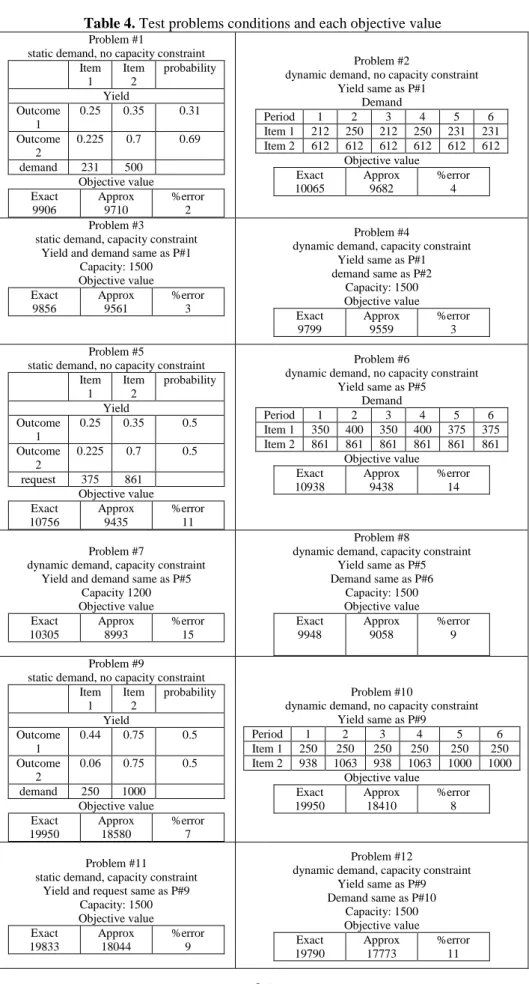
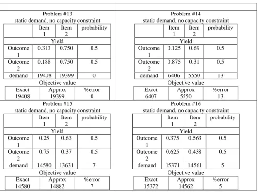
We suppose that the yields are stochastic in the first period and definite in the following periods. Consequently, we are collectingthe outcomes in periods other than the present period. For each period, we solve this estimated problem to determine the quantity of the product to be produced. Once the yields are obtained, they are allocated based on an assignment heuristic. The problemis solved, and the next period begins with new initial inventories and backorder states.Therefore, we solve the problem based on a finite horizon. We have tested the performance of the collection heuristic on a set of problems. To control the error caused by collection, we determined the objective value without any collection. The size of our test problems was greatly limited by the rate with which the size of the actual problem grows. The test problems consisted of two-product families. In each case, there were two possible outcomes for the yield, and the time horizon was 6 periods. To determine the expected profit from the collection procedure, we examined every possible set of yield outcomes over the horizon. Table 2 shows the features of the test problems. In this table, we illustrate the different request states and capacity conditions that we encounter in each problem.

Table 2. Test problems

Problem # demand condition Capacity condition

1 static No capacity constraint

2 static Capacity constraint

3 dynamic No capacity constraint

4 dynamic Capacity constraint

Thus, there are 16 issues in which we could precisely dissect the rough guess and % slip values for the target esteem in every issue. Note that the conditions are the same in every issue, i.e. creation cost: $10. The distinctive states of the issue are shown in tables 3 and 4.

(10)

Table 3. Test problem conditions Item 1 Item 2 Selling price 25 18.75 Backordering cost 2.5 1.875 Holding cost 1.25 1.25

Table 4. Test problems conditions and each objective value

Problem #1

static demand, no capacity constraint Item 1 Item 2 probability Yield Outcome 1

0.25 0.35 0.31

Outcome 2

0.225 0.7 0.69

demand 231 500

Objective value Exact 9906 Approx 9710 %error 2 Problem #2

dynamic demand, no capacity constraint Yield same as P#1

Demand

Period 1 2 3 4 5 6

Item 1 212 250 212 250 231 231 Item 2 612 612 612 612 612 612

static demand, capacity constraint Yield and demand same as P#1

Capacity: 1500 Objective value Exact 9856 Approx 9561 %error 3 Problem #4

dynamic demand, capacity constraint Yield same as P#1 demand same as P#2

0.25 0.35 0.5

Outcome 2

0.225 0.7 0.5

request 375 861 Objective value Exact 10756 Approx 9435 %error 11 Problem #6

Demand

Period 1 2 3 4 5 6

Item 1 350 400 350 400 375 375 Item 2 861 861 861 861 861 861

dynamic demand, capacity constraint Yield and demand same as P#5

Capacity 1200 Objective value Exact 10305 Approx 8993 %error 15 Problem #8

dynamic demand, capacity constraint Yield same as P#5 Demand same as P#6

0.44 0.75 0.5

Outcome 2

0.06 0.75 0.5

demand 250 1000

Period 1 2 3 4 5 6

Item 1 250 250 250 250 250 250

Item 2 938 1063 938 1063 1000 1000 Objective value Exact 19950 Approx 18410 %error 8 Problem #11 static demand, capacity constraint

Yield and request same as P#9 Capacity: 1500 Objective value Exact 19833 Approx 18044 %error 9 Problem #12

dynamic demand, capacity constraint Yield same as P#9 Demand same as P#10

Capacity: 1500 Objective value Exact 19790 Approx 17773 %error 11

26

(11)

Problem #13

static demand, no capacity constraint Item

1

Item 2

probability Yield

Outcome 1

0.313 0.750 0.5

Outcome 2

0.188 0.750 0.5

demand 19408 19399 0

Objective value Exact

19408

Approx 19399

%error 0

Problem #14

1 Item

2

probability Yield

Outcome 1

0.125 0.69 0.5 Outcome

2

0.875 0.31 0.5

demand 6406 5550 13

6407

Approx 5550

%error 13 Problem #15

1

Item 2

probability Yield

Outcome 1

0.25 0.63 0.5

Outcome 2

0.75 0.37 0.5

demand 14580 13631 7

14580

Approx 14882

%error 7

Problem #16

1

Item 2

probability Yield

Outcome 1

0.375 0.563 0.5

Outcome 2

0.625 0.438 0.5

demand 15371 14561 5

15372

Approx 14562

%error 5

The error in the objective value varies from 3% to 14%. The error increases with increasing variance in the yield. The variability in the products is greater in problems 5-9 than in problems 1-4. The errors in problems 1-4 are notably lower than those in problems 5 - 9. These numbers indicate that the error in the collection procedure is clearly affected by the variability in the yield. The effect of the yield variability on the quality of the heuristic solutions is further demonstrated by test problems 14, 15 and 16. The average yields are identical in these problems. However, the variability is largest in problem 15 and smallest in 17. The variation in the approximation error is consistent with the change in the variability. The summary of this analysis is illustrated in table 5.

Table 5. Test problems- Effect of field variability on error

Variance (problems 1- 4, in %) Variance (problems 5 - 9, in %)

Static demand 2 11

Dynamic demand 4 14

Stat. demand with cap. const. 3 15

Dyn. demand with cap. const. 3 9

5-1- Multi-family, capacitated problems

Until now, we have limited our consideration to a single-family problem. We now consider a multi-family problem and assume that we have a capacity constraint that limits the total quantity produced. In the absence of a capacity constraint, the problem can be separated by family, resulting in multiple single-family problems. We expand on a greedy procedure to solve the single-period problem. Because the capacity limitation affects all of the families, the size of constrained problems is notably larger than that of an unconstrained problem. For example, a single-period problem with eight families, each with ten customers and ten yield outcomes, will have 37500 constraints and 93750 variables. The number of constraints and variables grows exponentially with the number of families (Barbarosoglu and Özdamar, 2000).

The problem size increases equally quickly if we increase the number of periods. The problem size may become smaller if we relax the capacity constraint. Therefore, an obvious strategy is to relax the capacity constraint and use Lagrangian relaxation methods (Priyan and Uthayakumar 2014, Xanthopoulos, Koulouriotis et al. 2015). We choose this method, but we do not use linear programming to solve the resulting sub-problem. Instead, we expand a greedy procedure. At every stage of our algorithm, we compute the slight value to be used to assign an extra unit of production to a family. In the next section, we describe in considerable detail the algorithm for solving the single-period, multi-family constrained problem.

(12)

5-2- The Greedy Procedure for a Single-period Problem

The multi-family, constrained problem is given by the following.

∑

= =

−

=

F f f f F f f f f f a f

o

G

u

m

I

C

m

S

I

F

1 1 , 1 , 1 1 , 1 1

1

(

,

π

)

max

(

,

π

)

S.T.

∑

=

≤

F f f

C

m

1

m_f ≥0.

(28)

The index f indicates the family. The function SoGf,1(.) represents the assumed value of the evening

problem for family f. The framework of the evening problems in the multi-family, single-period case is similar to that of the evening problem for the single-family case. Because each S_oG_f_,₁(.) is a concave function whose value depends only on mf, with a different value of m for i≠ f , the capacitated problem is a concave knapsack problem. As a result, the optimal technique is a greedy procedure that assigns the next unit of production to the family with the highest slight profit. Below, we define an approximation procedure that assigns

δ

units of production at each step of the assignment process.

STEP 1: initialize.

Calculate _f

f m f C f m f G o S f γ

λ =[∂ _,₁(.,.)/∂ − ] = 0

=

∀f

γ

f , where f

λ

= a slight value used to assign a unit of production to family j and f

γ

= the capacity assigned to family f.

STEP 2: identify the family with the highest slight value.

f* = ArgMax[λ_f ]; If

λ

_f* ≤0 STOP (optimality condition) STEP 3: assign production to family f*.

e f f* =γ * + ′′

γ , where e′= min {where e denotes the unassigned capacity} STEP 4: check if the capacity has been entirely assigned. If so, STOP.

STEP 5: update the slight value for family f*. Calculate * * ] * * / (.,.) 1 , * [ * f q f m f c f m f G o S

f = ∂ ∂ − =

λ .

Return to Step 2.

For e>0, this procedure is an approximation procedure. The final solution may not be optimal. We describe a procedure for calculating

λ

f below.

Analyze a family, f, and let

α

mf be the probability of observing that a yield outcome of m. Then,

) , 2 , 2 ( ) , 1 , 1 ( ] / ,.) (., 1 , [

1 [ ,1(., ,.)/ ] ] / ,.) (., 1 , [ f m u f m f m u f m f f m f m f a u f G f M

m mf Cf mf f

f a u f G f m f f m f C f m f a u f G o S f ω ω γ γ α γ λ + = = ∂ ∂ ∑ = ∂ ∂ − = = = − ∂ ∂ = ,

Where

ω

₁f_,_m and

ω

₂f_,_m are the shadow prices of constraints 2 and 3, respectively, with m_f =

γ

_f. These shadow prices can be specified by solving the corresponding linear program and can also be calculated exactly.

ω

_if_,_m is the slight value of an extra unit of item i, given the manufacture of m_f units with an outcome of m. Because we realize the yield, we can specify how the next unit of item i will be used and its

(13)

value under the optimal assignment process. For example, if m_fu₁f_,_m is less than the request by customer l, the value of the next unit of item 1 would be equal to the selling price plus the backorder penalty for customer 1.

u

_1,f_mis the yield of item 1 of family f under outcome m. An algorithm for specifying the shadow prices by assigning the items to the customers is shown in Figure 3.

Figure 3. Algorithm to compute the shadow price

We begin with customer 1 and go down the scale. For customer c, we first assign item k. If the yield of item c is sufficient, the shadow price for item k is the same as its rescue value. If the demand of customer c cannot be fulfilled by item c, the shadow price of item c is set equal to the selling price plus the backorder cost of customer c. We then move up the scale (beginning from item c-1) to see if we can assign item c-i

) 1 1

( ≤i≤c− to customer c. Before we demote item c-i, we must check the following. (a) Whether there are any excesses of item c-i and

(b) Whether the selling price plus the backorder cost for customer c surpasses the rescue price of item c-i. We assign item c-i to customer c only if the answer to both the questions is yes. If we demote, the shadow price of item c-i is updated. The item can have two new shadow prices.

(1) If the excess quantity of item c-i is equals to or exceeds the residual needs of customer c, the shadow prices of items c-i through c are set equal to the rescue price of item c.

(2) If the excess quantities of items c-i are insufficient, the shadow prices of item c-i are set to the selling prices plus the backorder cost for customer c.

Compute output of all items

k=1

Allocate item k to customer k

Demand of k met? Item k shadow price=item k salvage value

Item k shadow price=customer k selling price+backorder cost yes

no START

j=k-1 k=k+1

j=0

salvage value of item j>selling +backorder cost of customer k?

k=k+1

stocks of item j available?

allocate item j to customer k. item j shadow price= customer k selling price+backorder cost

Demand for customer j backordered?

Customer k's demand met?

j=j-1

for items j to k shadow price=salvage value of j no

yes

no no

END j>0

no

1 yes

1

yes

(14)

The demoting process for customer c is ended if (1) the rescue price of item c-i is greater than the selling price plus the backorder cost for customer c or (2) there are no more excesses.

The algorithm requires O(M_fZ2_f ) steps to calculate

λ

_f, where Mf is the number of outcomes for family f, and Zf is the number of items in family f.

6- Conclusions

In this paper, we have modeled a production-planning problem based on a real case in the electronic industry. The most important aspect of this work was recognizing andbuilding the problem. In this area, the yields vary notably, and the demandsare changeable. In addition, differentitems may be received from each production lot. We have formulated the problem as a probabilistic one. Based on the framework of a two-period problem, we have determined a class of heuristicsto assign items to customers. The heuristics assign items to customers in a way that keeps the net demands for the items in equilibrium. The aim of the heuristics is to prevent the net demand for any item from surpassing the predetermined level of the total demand for all of the items. These assignment strategies are characteristic of the yield possibilities with multiplicative yields.

We also assume approximation procedures to solve single-family limited horizon problems with and without capacity constraints. We approximate the problem by assuming that the yields are definite in all but the first period on the horizon. We have tested this procedure on sample problems. The size of the test problems was restricted by the size of the specific problems. The errors in the objective value varied between 3% and 14%. The possibility ranking in the yield had a significant effect on the performance of the heuristic procedure. We have established a greedy procedure for solving the single-period, multi-family capacitated problem.

Finally, we consider a real world problem that introduces a risk-based method that combines Monte Carlo simulation with traditional method to evaluate and support in choosing the best RE plan given sustainability analyses. The proposed method does not need criteria weighting or accurate quantitative computation as it clarifies the decision making process by solving problems relied on qualitative or quantitative information.

References

Adacher, L. and C. G. Cassandras (2014). "Lot size optimization in manufacturing systems: The surrogate method." International Journal of Production Economics 155(0): 418-426.

Adulyasak, Y., J.-F. Cordeau and R. Jans (2015). "The production routing problem: A review of formulations and solution algorithms." Computers & Operations Research 55(0): 141-152.

Ashayeri, J., N. Ma and R. Sotirov (2015). "The redesign of a warranty distribution network with recovery processes." Transportation Research Part E: Logistics and Transportation Review 77(0): 184-197.

Barattieri, A. (2014). "Comparative advantage, service trade, and global imbalances." Journal of International Economics 92(1): 1-13.

Barbarosoglu, G. and L. Özdamar (2000). "Analysis of solution space-dependent performance of simulated annealing: the case of the multi-level capacitated lot sizing problem " Computers & Operations Research 27(9): 895-903 .

Birge, J. R. and R. J.-B. Wets (1986). "Designing approximation schemes for stochastic optimization problems, in particular for stochastic for stochastic programs with recourse." Mathematical Programming Study 27: 54-102.

Bitran, G. R. and D. Tirupati (1988). "Planning and scheduling for epitaxial wafer production facilities." Operarions Research 36: 34-49.

Capaldo, A. and I. Giannoccaro (2015). "Interdependence and network-level trust in supply chain networks: A computational study." Industrial Marketing Management 44(0): 180-195.

(15)

Chang, H., H. Jula, A. Chassiakos and P. Ioannou (2008). "A heuristic solution for the empty container substitution problem." Transportation Research Part E: Logistics and Transportation Review 44(2): 203-216.

Chang, X., H. Xia, H. Zhu, T. Fan and H. Zhao (2015). "Production decisions in a hybrid manufacturing– remanufacturing system with carbon cap and trade mechanism." International Journal of Production Economics 162(0): 160-173.

Chen, J.-F. (2003). "Component allocation in multi-echelon assembly systems with linked substitutes." Computers & industrial engineering 45(1): 43-60.

Chew, E. P., C. Lee, R. Liu, K.-s. Hong and A. Zhang (2014). "Optimal dynamic pricing and ordering decisions for perishable products." International Journal of Production Economics 157(0): 39-48.

Chung, Y. and A. Heshmati (2015). "Measurement of environmentally sensitive productivity growth in Korean industries." Journal of Cleaner Production 104(0): 380-391.

Coad, A. F. and J. Cullen (2006). "Inter-organisational cost management: Towards an evolutionary perspective." Management Accounting Research 17(4): 342-369.

Crevier, B., J.-F. Cordeau and G. Laporte (2007). "The multi -depot vehicle routing problem with inter-depot routes " European Journal of Operational Research 176(2): 756-773 .

Dantzig, G. B. (1955). "Linear programming under uncertainty." Management Science 1: 197-206.

Dasgupta, S. and J. Roy (2015). "Understanding technological progress and input price as drivers of energy demand in manufacturing industries in India." Energy Policy 83(0): 1-13.

De Mazancourt, C. and M. W. Schwartz (2010). "A resource ratio theory of cooperation." Ecology letters 13(3): 349-359.

Deuermeyer, B. L. and W. P. Pierskalla (1978). "A by-product production system with an alternative." Management Science 24(13): 1373-1383.

Eğilmez, G. and G. A. Süer (2015). "Stochastic cell loading to minimize nT subject to maximum acceptable probability of tardiness." Journal of Manufacturing Systems 35(0): 136-143.

Elbanhawi, M. and M. Simic (2014). "Randomised kinodynamic motion planning for an autonomous vehicle in semi-structured agricultural areas." Biosystems Engineering 126(0): 30-44.

Fagerholt, K., N. T. Gausel, J. G. Rakke and H. N. Psaraftis (2015). "Maritime routing and speed

optimization with emission control areas." Transportation Research Part C: Emerging Technologies 52(0): 57-73.

Feng, C.-M., P.-J. Wua and K.-C. Chia (2010). "A hybrid fuzzy integral decision-making model for locating manufacturing centers in China: A case study " European Journal of Operational Research 200(1): 63-73.

Flapper, S. D., J.-P. Gayon and L. L. Lim (2014). "On the optimal control of manufacturing and

remanufacturing activities with a single shared server." European Journal of Operational Research 234(1): 86-98.

Fujimoto, T. and Y. W. Park (2014). "Balancing supply chain competitiveness and robustness through “virtual dual sourcing”: Lessons from the Great East Japan Earthquake." International Journal of Production Economics 147, Part B(0): 429-436.

Gallego, G., K. Katircioglu and B. Ramachandran (2006). "Semiconductor inventory management with multiple grade parts and downgrading." Production Planning & Control 17(7): 689-700.

(16)

Hosoda, T., S. M. Disney and S. Gavirneni (2015). "The impact of information sharing, random yield, correlation, and lead times in closed loop supply chains." European Journal of Operational Research 246(3): 827-836.

Jane, C.-C. and Y.-W. Laih (2005). "A clustering algorithm for item assignment in a synchronized zone order picking system " European Journal of Operational Research 166(2): 489-496.

Jin, X. (2012). Modeling and Analysis Of Remanufacturing Systems with Stochastic Return and Quality Variation, General Motors Company.

Karaesmen, I. and G. Van Ryzin (2004). "Overbooking with substitutable inventory classes." Operations Research 52(1): 83-104.

Karlo, A. H. and M. M. Gohil (1982). "A lot size model with backlogging when the amount received is uncertain." Internatioal Journal of Production Research 20: 775-786.

Lee, C. Y. and T. Lu (2015). "Inventory competition with yield reliability improvement." Naval Research Logistics (NRL) 62(2): 107-126.

Lee, J. (2014). "Dynamic pricing inventory control under fixed cost and lost sales." Applied Mathematical Modelling 38(2): 712-721.

Lee, S.-c., D.-h. Oh and J.-d. Lee (2014). "A new approach to measuring shadow price: Reconciling engineering and economic perspectives." Energy Economics 46(0): 66-77.

Li, H. and N. K. Womer (2015). "Solving stochastic resource-constrained project scheduling problems by closed-loop approximate dynamic programming." European Journal of Operational Research 246(1): 20-33.

Lin, J. T. and C.-M. Chen (2015). "Simulation optimization approach for hybrid flow shop scheduling problem in semiconductor back-end manufacturing." Simulation Modelling Practice and Theory 51(0): 100-114.

Lin, J. T. and C.-J. Huang (2014). "A simulation-based optimization approach for a semiconductor photobay with automated material handling system." Simulation Modelling Practice and Theory 46(0): 76-100.

Mak, H. Y. and Z. J. M. Shen (2009). "A two‐echelon inventory‐location problem with service considerations." Naval Research Logistics (NRL) 56(8): 730-744.

Martagan, T. and B. Ekşioğlu (2013). "Game theoretic analysis of an inventory problem with substitution, stochastic demand, and uncertain supply." International Journal of Inventory Research 2(1-2): 27-43.

Mazzolla, J., F. W. McCoy and H. M. Wagner (1987). "Algorithms and heuristics for variable yield lot sizing." Naval Research Log Quartely 34: 67-86.

Melouk, S. H., B. A. Fontem, E. Waymire and S. Hall (2014). "Stochastic resource allocation using a predictor-based heuristic for optimization via simulation." Computers & Operations Research 46(0): 38-48.

Mohammadi, M., S. N. Musa and A. Bahreininejad (2015). "Optimization of economic lot scheduling problem with backordering and shelf-life considerations using calibrated metaheuristic algorithms." Applied Mathematics and Computation 251(0): 404-422.

Mookherjee, R. and T. L. Friesz (2008). "Pricing, allocation, and overbooking in dynamic service network competition when demand is uncertain." Production and Operations Management 17(4): 455-474.

Olsen, P. (1976). "Multistage stochastic program with recourse: the equivalent deterministic problem." SIAM Journal on Computing and Optimization 14: 495-517.

(17)

Osterloff, M. (2003). "Technology-based product market entries: managerial resources and decision-making process."

Polyakovskiy, S. and R. M'Hallah (2014). "A multi-agent system for the weighted earliness tardiness parallel machine problem." Computers & Operations Research 44(0): 115-136.

Ponsignon, T. and L. Mönch (2014). "Simulation-based performance assessment of master planning approaches in semiconductor manufacturing." Omega 46(0): 21-35.

Priyan, S. and R. Uthayakumar (2014). "Optimal inventory management strategies for pharmaceutical company and hospital supply chain in a fuzzy–stochastic environment." Operations Research for Health Care 3(4): 177-190.

Rajaram, K. and C. S. Tang (2001). "The impact of product substitution on retail merchandising." European Journal of Operational Research 135(3): 582-601.

Rotondo, A., P. Young and J. Geraghty (2015). "Sequencing optimisation for makespan improvement at wet-etch tools." Computers & Operations Research 53(0): 261-274.

Safaei, M. and K. D. Thoben (2014). "Measuring and evaluating of the network type impact on time uncertainty in the supply networks with three nodes." Measurement 56(0): 121-127.

Samsatli, S., N. J. Samsatli and N. Shah (2015). "BVCM: A comprehensive and flexible toolkit for whole system biomass value chain analysis and optimisation – Mathematical formulation." Applied Energy 147(0): 131-160.

Sarkar, B., B. Mandal and S. Sarkar (2015). "Quality improvement and backorder price discount under controllable lead time in an inventory model." Journal of Manufacturing Systems 35(0): 26-36.

Sethi, S. P., M. Taksar and Q. Zhang (1995). "Hierarchical capacity expansion and production planning decisions in stochastic manufacturing systems." Journal of Operations Management 12(3-4): 331-352.

Shih, W. (1980). "Optimal inventory policies when stockout results from defective products." Internatioal Journal of Production Research 18: 677-686.

Shin, H., S. Park, E. Lee and W. C. Benton (2015). "A classification of the literature on the planning of substitutable products." European Journal of Operational Research 246(3): 686-699.

Silver, E. A. (1976). "Establishing the reorder quantity when the amount received is uncertain." INFOR 14: 32-39.

Song, L. (2009). "Supply Chain Management with Demand Substitution." Doctoral Dissertations: 91.

Sprenger, R. and L. Mönch (2014). "A decision support system for cooperative transportation planning: Design, implementation, and performance assessment." Expert Systems with Applications 41(11): 5125-5138.

Tan, S. T., C. T. Lee, H. Hashim, W. S. Ho and J. S. Lim (2014). "Optimal process network for municipal solid waste management in Iskandar Malaysia." Journal of Cleaner Production 71(0): 48-58.

Varas, M., S. Maturana, R. Pascual, I. Vargas and J. Vera (2014). "Scheduling production for a sawmill: A robust optimization approach." International Journal of Production Economics 150(0): 37-51.

Veinott, A. F. (1960). "Stattus of mathematical inventory theory." Management Science 11: 745-777.

Xanthopoulos, A. S., D. E. Koulouriotis and P. N. Botsaris (2015). "Single-stage Kanban system with deterioration failures and condition-based preventive maintenance." Reliability Engineering & System Safety 142(0): 111-122.

(18)

Yao, S., Z. Jiang, N. Li, H. Zhang and N. Geng (2011). "A multi-objective dynamic scheduling approach using multiple attribute decision making in semiconductor manufacturing " International Journal of Production Economics 130(1): 125-133.

Yeh, K., M. J. Realff, J. H. Lee and C. Whittaker (2014). "Analysis and comparison of single period single level and bilevel programming representations of a pre-existing timberlands supply chain with a new biorefinery facility." Computers & Chemical Engineering 68(0): 242-254.

Zhang, G. and X. Wang (2014). "Dual-Channel Supply Coordination in Online Shopping." Procedia CIRP 17(0): 617-621.

Zhang, J., W. Qin, L. H. Wu and W. B. Zhai (2014). "Fuzzy neural network-based rescheduling decision mechanism for semiconductor manufacturing." Computers in Industry 65(8): 1115-1125.

Zhang, T., Q. P. Zheng, Y. Fang and Y. Zhang (2015). "Multi-level inventory matching and order planning under the hybrid Make-To-Order/Make-To-Stock production environment for steel plants via Particle Swarm Optimization." Computers & Industrial Engineering 87(0): 238-249.

Zhu, Y., Y. P. Li and G. H. Huang (2015). "An optimization decision support approach for risk analysis of carbon emission trading in electric power systems." Environmental Modelling & Software 67(0): 43-56.