Development of a new integrated method for generation IDF curves based on three climatic changes scenarios

(1)

Sharif University of Technology

Scientia Iranica

Transactions A: Civil Engineering http://scientiairanica.sharif.edu

Development of a new integrated method for

generation of IDF curves based on three scenarios of

climatic changes

A. Adib

_{and S. Ghafari Rad}

Department of Civil Engineering, Faculty of Engineering, Shahid Chamran University of Ahvaz, Iran. Received 11 June 2017; received in revised form 24 July 2017; accepted 3 November 2017

KEYWORDS Climatic change; The HadCM3; IDF curves; RBF ANN; The Baghmalek climatic station; The Gumbel distribution.

Abstract. Climate change can change the Intensity-Duration-Frequency (IDF) curves. This research study evaluates IDF curves changes of the Baghmalek climatic station in the southwest of Iran. A developed integrated method extracted the IDF curves using the Gumbel and log-Pearson III probability distributions and observed maximum annual precipitations. Durations of these precipitations are 15, 30, 45 minutes and 1,2,3,6 and 12 hours. For this purpose, this method utilizes the recorded precipitation data of the Baghmalek climatic station in a 40-year period (1974-2013). Then, mean square error method determines the probability distribution that has the best tting with this data. The HadCM3 prepares precipitation data for a 30-year period (2021-2050) based on A1B, B1, and A2 scenarios. In addition, this method selects an optimum articial neural network to extract maximum annual rainfall intensity for dierent durations and scenarios. Then, selected network and the chosen probability distribution produce IDF curves for dierent return periods and scenarios. Produced IDF curves for dierent scenarios are compared to IDF curves of a base time period. Because of increasing carbon dioxide and its greenhouse eects in these scenarios, rainfall intensity will increase for return periods less than 2.33 years, while it will decrease for return periods more than 2.33 years.

1. Introduction

In recent decades, high growth rate of population and industrialization of human societies have increased the concentration of greenhouse gases as dioxide carbon in the atmosphere, which changed mean, maximum, and minimum temperature as well as average annual precipitation in dierent countries. Because of special weather conditions and large oil resources in the Middle East, eects of climatic changes on these countries are

*. Corresponding author.

E-mail address: [email protected] (A. Adib); saeid [email protected] (S. Ghafari Rad) doi: 10.24200/sci.2017.4593

greater than those on other countries are. For example, Khuzestan province in the southwest of Iran has the largest oil resources and steel industries available in Iran. This province is Iran's industrial center. Because of climatic changes in recent years, severe dust storms often occur in this province. Intensity of these storms is unprecedented, starting from 2006. Climatic changes can aect hydrologic characteristics of dierent water-sheds; for example, IDF curves can change.

This research has three dierent aspects (gen-eration of IDF curves, use of General Circulation Model (GCM), and investigation of eects of climatic changes on IDF curves), while other researchers usually consider one or two aspects in their studies. To study IDF curves and use probability distributions or empirical relationships for generation of these curves,

(2)

A. Adib and S. Ghafari Rad/Scientia Iranica, Transactions A: Civil Engineering 26 (2019) 742{751 743

the research studies such as: Garcia-Bartual and Schneider [1] in Spain, Yu et al. [2] in Taiwan, Madsen et al. [3] in Denmark, Agilan and Umamahesh [4] in India, Huang et al. [5] in Malaysia, Fadhel et al. [6] in England, and Bezak et al. [7] in Slovenia should be consulted. Yu et al. [2] used scaling theory and Gumbel probability distribution to generate regional IDF formulas at 46 rain gauge stations of northern Taiwan. They considered annual 1-day maximum series for scaling theory. In their research, the study area was divided into three homogenous regions. Their results showed that the regional IDF scaling formulas proposed suitable results in simulation and verication. Khan et al. [8] in Canada, Wang and Lau [9] in United State of America (USA), Hashmi et al. [10] in New Zealand, and Gulacha and Mulungu [11] in Tan-zania utilized GCM and dierent downscaling meth-ods to predict future climatic data (such as rainfall, temperature, etc.). Gulacha and Mulungu [11] utilized the Statistical Down Scaling Model (SDSM) for down-scaling of prepared data by GCM model in the Wami-Ruvu River Basin. They considered the base time period of 1961-1990 and used the HadCM3 to prepare precipitation and temperature data in the 2020 s, 2050 s, and 2080 s based on B2 and A2 scenarios. They showed that annual and monthly precipitation and maximum temperature would increase and minimum temperature would decrease or increase in the future.

In addition, Kuok et al. [12] in Malaysia, Mailhot et al. [13] in Canada, Alam and Elshorbagy [14] in Canada, Kuo et al. [15] in Canada, Lima et al. [16] in Korea, Agilan and Umamahesh [17] in India, Si-monovic et al. [18] in Canada, and DeGaetano and Castellano [19] in U.S.A. applied GCM and dierent downscaling methods to generation of IDF curves. Mailhot et al. [13] applied the Canadian Regional Climate Model (CRCM) to evaluate eects of climatic changes on IDF curves (from 2041 to 2070) in Southern Quebec. The base time period of this research was 1961-1990. They considered annual maximum rainfall data time series from May to October, and durations of precipitation included 2, 6, 12, and 24 hours. They showed that return periods of 2-, 6-, 12-, and 24-h rainfall events (for constant rainfall intensity) would decrease in the future.

This study develops a new integrated method (using GCM model, RBF neural network, and dierent probability distributions) to generate IDF curves of dierent scenarios of climatic changes that may occur in the future. For this purpose, this method utilized generated data by a GCM and a RBF articial neu-ral network. The HadCM3 (Hadley Centre Coupled Model, version 3) and RBF-ANN generate maximum annual rainfall intensity for dierent durations and scenarios in the next years. At the end, a suitable probability distribution (Gumbel probability

distribu-tion) produces IDF curves. Most research studies use rainfall-runo models to extract necessary information from generated data by GCM; however, this study utilizes a RBF-ANN for this purpose. This study takes the following steps:

1. Preparation of precipitation data in a 40-year pe-riod (1974-2013) and determination of IDF curves using a suitable probability distribution;

2. Extraction of climatic data using HadCM3 model for three scenarios (A1B, B1, and A2) in a 30-year period (2021-2050);

3. Determination of maximum annual rainfall inten-sity for dierent durations and scenarios in the next years (2021-2050) using extracted data by HadCM3 model and a suitable RBF ANN;

4. Determination of IDF curves of three scenarios using selected probability distribution in step 1;

5. Comparison of IDF curves of three scenarios and IDF of the base time period (1974-2013).

2. Materials and methods 2.1. Case study

The Baghmalek is a city in Khuzestan province, lo-cated in southwestern part of Iran. The Baghmalek watershed is a part of the Zard River watershed. The Zard River is a tributary of the Jarahi River. The Baghmalek watershed is located between 49₃₉0 _to

50₁₁0 _{E longitude and 31}₂₂0 _{to 31}₄₂0 _{N latitude.}

The area of this watershed is 884 km2_{. Maximum,}

mean, and minimum heights of this watershed are 3303.3, 1197, and 391.7 m, respectively. Mean an-nual temperature and precipitation rates are 27_and

450 mm, respectively. Figure 1 illustrates Baghmalek watershed and its location in Khuzestan province, Iran. 2.2. Research methodology

2.2.1. The HadCM3 (Hadley centre Coupled Model, version 3)

The HadCM3 is a coupled atmosphere-ocean general circulation model (AOGCM). This model was devel-oped at the Hadley Centre in the United Kingdom and has two components (the atmospheric model HadAM3 and the ocean model HadOM3). The HadOM3 has a sea ice model. In addition, this model does not need to do ux adjustment to improve simulation. For simulation, this model assumes that the number of days in a year is 360 days (each month is 30 days). Advantages of this model include high resolution of HadOM3 and good coordination between HadOM3 and HadAM3 [21-23].

(3)

Figure 1. The Baghmalek watershed and its location in Khuzestan province, Iran [20].

2.2.2. The Special Report on Emissions Scenarios (SRES)

The Intergovernmental Panel on Climate Change (IPCC) published a report (SRES) in 2000. This report described scenarios concerning greenhouse gas emission. These scenarios can be used to predict climatic changes in the future. In addition, IPCC published the IPCC Third Assessment Report (TAR) in 2001 and the IPCC Fourth Assessment Report (AR4) in 2007. TAR and AR4 described four scenarios (A1, A2, B1, and B2). In this research, three scenarios have considered A1B, B1, and A2. The A1 scenario family predicts the following:

1. A very rapid growth of economy in the future;

2. The peak of global population to occur in the mid-century;

3. A decrease in population after the mid-century. In this scenario, new and more ecient technolo-gies will develop very rapidly. Dierences in the income per capita between developed and developing countries will reduce, and cultural and social interactions will increase among dierent regions of the world. The A1 scenario family is divided into three groups, which are dependent on technological change in the energy system. The three A1 groups include fossil intensive (A1FI), non-fossil energy sources (A1T), or a balance across all sources (A1B).

The A2 scenario family predicts a very heteroge-neous world. Characteristics of this scenario include self-reliance and preservation of local identities. The

population is increasing continuously. Economic devel-opment is not global and is dierent in developed and developing countries. Per capita economic growth and technological change are more fragmented and slower than other scenarios.

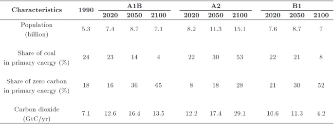
The B1 scenario family predicts a convergent world. The peak of global population is in mid-century and will decrease after the mid-mid-century (as the A1 scenario); however, with rapid changes will be observed in economic structures toward a service and information economy, a reduction in material intensity, and application of clean and resource-ecient technolo-gies. The purpose of this scenario is to present global solutions for economic, social, and environmental sus-tainability, including improved equity, yet without additional climate initiatives. The characteristics of three scenarios are shown in Table 1.

2.2.3. RBF ANN

Radial base function network is a suitable ANN for su-pervised learning problems as regression, classication, and time series prediction. This network has usually three layers:

1. Input layer. In this layer, the number of nodes is equal to that of datasets. Input layer in this research has two nodes (annual precipitation depth and mean annual temperature are data sets).

2. Hidden layer. In this layer, the optimum number of nodes and its parameters must be determined by trial-error method. This layer develops a nonlinear adaptation between inputs and outputs

(4)

Table 1. The characteristics of three scenarios A1B, B1, and A2 [24].

Characteristics 1990 A1B A2 B1

2020 2050 2100 2020 2050 2100 2020 2050 2100 Population

(billion) 5.3 7.4 8.7 7.1 8.2 11.3 15.1 7.6 8.7 7

Share of coal

in primary energy (%) 24 23 14 4 22 30 53 22 21 8

Share of zero carbon

in primary energy (%) 18 16 36 65 8 18 28 21 30 52

Carbon dioxide

(GtC/yr) 7.1 12.6 16.4 13.5 12.2 17.4 29.1 10.6 11.3 4.2

and converts nonlinear patterns to separable linear patterns. This layer utilizes a nonlinear activation function. This function is:

F (x) =

N

X

i=1

wih(kx uik); (1)

where N is the number of neurons in the hidden layer, ui is the center vector for neuron i, and wi is

the weight of neuron i in the linear output neuron. The radial basis function is commonly Gaus-sian basis function.

h(kx uik) = exp

kx uik2

i

; (2)

where i is the Kernel weight factor for neuron i.

3. Output layer. This layer produces a linear combi-nation from wi. The number of the nodes is equal

to that of outputs of network. In this research, this layer has one node (maximum intensity of rainfall for each duration is output of ANN).

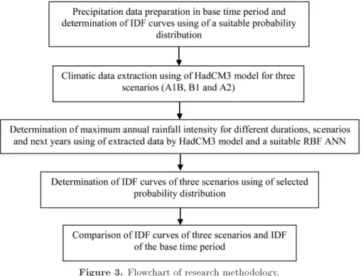
Figure 2 shows a RBF ANN and Figure 3 shows a owchart of research methodology.

3. Results and discussion

Results of this study are stated in the following steps:

Figure 2. A radial base function articial neural network [25].

Step 1: Preparation of precipitation data in base time period and determination of IDF curves using a suitable probability distribution. Khuzestan Water and Power Authority (KWPA) has recorded the depth of occurred rainfalls in 15-minute time steps at the Baghmalek climatic station. These rainfalls occurred in a 40-year period (1974-2013). By using such recorded data, maximum annual intensity of precipitation was extracted for dierent durations (15, 30, and 45 min-utes and 1, 2, 3, 6, and 12 hours). Table 2 illustrates

Table 2. The minimum, mean and maximum values of maximum annual intensity of precipitation for dierent durations. Duration 15 min 30 min 45 min 1 hour 2 hours 3 hours 6 hours 12 hours

Min (mm/hr) (year)

16.8 (2013)

8.4 (2004)

5.6 (2004)

5.1 (2004, 2013)

2.55 (2004)

1.7 (2004)

0.61 (2013)

0.7 (1999) Mean (mm/hr) 133.35 68.89 49.7 37.62 23.09 14.14 4.9 3.06

Max (mm/hr) (year)

583.20 (2010)

291.60 (2010)

194.53 (2010)

145.90 (2010)

73.05 (2010)

46.83 (1994)

20.48 (1994)

10.45 (1994)

(5)

Figure 3. Flowchart of research methodology.

Table 3. Rainfall intensity (mm/hr) for dierent durations and return periods (1974-2013). Probability

distribution

Return period (year)

Duration (min)

15 30 45 60 120 180 360 720

Gumbel

2 117.08 61.02 44.40 33.64 20.67 12.72 4.31 2.76 2.3 129.03 66.80 48.29 36.56 22.44 13.77 4.74 2.98 100 489.39 241.08 165.65 124.55 75.96 45.35 17.70 9.83

Log pearson III

2 53.81 31.63 23.87 18.18 11.20 6.92 2.37 1.62 2.3 113.47 73.47 77.93 51.92 34.16 18.76 6.18 2.76 100 420.39 189.16 121.79 96.36 58.36 35.99 12.27 7.85 Table 4. MSE (mm/hr)2 _{of Gumbel and log pearson III probability distributions.}

Probability distribution

Duration (min)

15 30 45 60 120 180 360 720

Gumbel 17.19 5.3 3.56 2.81 4.98 3.16 1.63 0.52 Log pearson III 18 7.91 4.9 4.02 4.01 2.68 1.56 0.61

the minimum, mean, and maximum values of maximum annual intensity of precipitation.

To extract IDF curves and determine rainfall intensity for each duration and return period, two conventional probability distributions (Gumbel and log pearson III) were tested by mean square error method. MSE of these distributions was calculated for observed data in the base time period (1974-2013). Table 3 shows calculated rainfall intensity by two probability distributions for dierent durations and return periods

in base time period. Table 4 shows MSE of calculated values by two probability distributions.

For most of durations, MSE of the Gumbel proba-bility distribution is lower than that of the log pearson III probability distribution. Moreover, for durations with low MSE of the log pearson III probability distri-bution, the dierence between MSE of this distribution and MSE of the Gumbel probability distribution is negligible. Therefore, to prepare IDF curves, the Gum-bel probability distribution is a suitable distribution.

(6)

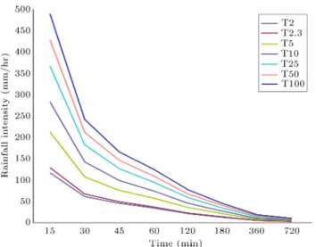
Figure 4. Produced IDF curves using the Gumbel probability distribution (1974-2013).

Therefore, this probability distribution uses production of IDF curves from 1974 to 2013 (Figure 4).

Step 2: Training, validation, and testing of RBF ANN and selection of its optimum parameters. For selection of the optimum values of parameters (number of nodes in hidden layer and the Kernel weight factor), RBF ANN must be trained using observed data in base time period (1974-2013). Annual precipitation depth and mean annual temperature (240 = 80 inputs) were introduced to ANN, and outputs included maximum annual rainfall intensity of dierent durations (408 = 320 outputs), calculated by ANN. Then, 70, 15 and 15 percents of data were applied to training, validation, and testing of ANN, respectively. RBF ANNs with dierent number of nodes in hidden layer and the Kernel weight factors were evaluated, whose results are shown in Table 5.

The MSE changes of selected RBF ANN and eects of changes of the number of nodes in hidden layer and the Kernel weight factor on MSE are illustrated in Figures 5 to 7.

Maximum annual rainfall intensity was calculated by selected RBF ANN for dierent durations (15, 30, and 45 minutes and 1, 2, 3, 6, and 12 hours) in base time period. Table 6 shows the minimum, mean, and maximum values of calculated maximum annual

Figure 5. Eects of changes of the number of nodes in hidden layer on MSE.

Figure 6. Eects of changes of the Kernel weight factor on MSE.

Figure 7. The MSE changes of selected RBF ANN.

rainfall intensity by selected RBF ANN for dierent durations.

Step 3: Climatic data extraction using the HadCM3 model for three scenarios (A1B, B1, and A2): In this research, annual precipitation depth and mean annual temperature have been extracted using the HadCM3

Table 5. The optimum values of parameters of RBF ANN for dierent durations. Durations (min) 15 30 45 60 120 180 360 720

Number of nodes

in hidden layer 100 99 99 100 100 100 100 100 The Kernel

(7)

Table 6. The minimum, mean, and maximum values of maximum annual rainfall intensity for dierent durations (calculated by selected RBF ANN).

Duration 15 min 30 min 45 min 1 hour 2 hours 3 hours 6 hours 12 hours Min (mm/hr)

(year)

17 (2013)

8.5 (2004)

5.3 (2004)

5.15 (2004, 2013)

2.3 (2004)

1.9 (2004)

0.7 (2013)

0.65 (1999)

Mean (mm/hr) 123.86 62.7 45.68 34.61 21.7 13.81 4.92 3.05

Max (mm/hr) (year)

545.3 (2010)

323.5 (2010)

172.4 (2010)

165 (2010)

80.4 (2010)

45.1 (1994)

21.2 (1994)

12.14 (1994) Table 7. The minimum, mean, and maximum values of

extracted annual precipitation depth and mean annual temperature for three scenarios (2021-2050).

Scenarios A1B B1 A2

Annual precipitation depth (mm)

Min 143.63 189.44 72.67 Mean 348.78 383.59 346.86 Max 575.75 621.16 589.84

Mean annual temperature (_C)

Min 16.19 15.6 16.31 Mean 17.83 17.23 17.7 Max 19.57 18.75 19.01

model and the AR4(2007) assessment. The three considered scenarios are B1, A2, and A1B. Annual precipitation depth and mean annual temperature of three scenarios are illustrated in Table 7.

Step 4: Determination of maximum annual rainfall intensity for dierent durations and scenarios in the next years (2021-2050) using RBF ANN and deter-mination of IDF curves of three scenarios using the Gumbel probability distribution. IDFs of three scenarios are illustrated in Table 8.

Step 5: Comparison of IDF curves of three scenar-ios with IDF of the base time period. IDF curves of three scenarios and the base time period have been compared, and the results have been observed.

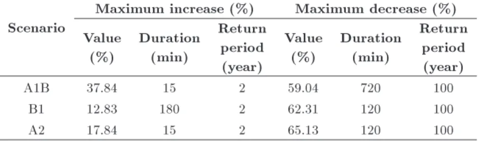
In comparison with IDF curves of the base time period, Table 9 and Figures 8 to 10 illustrate that rainfall intensity increases for dierent durations and scenarios (return periods less than 2.3 years), while it decreases for dierent durations and scenarios (return periods more than 100 years). Due to increasing greenhouse gases (especially dioxide carbon) in the future, the number of regular rainfalls will increase and the number of heavy rainfalls will decrease. This study presents the reason for increasing rainfall intensity of return periods less than 2.3 years and decreasing rainfall intensity of return periods more than 2.3 years. From 2021 to 2050, the volume of dioxide carbon

Figure 8. Comparison of rainfall intensity of three scenarios and the base time period for dierent durations (return period 2 years).

Figure 9. Comparison of rainfall intensity of three scenarios and the base time period for dierent durations (return periods 2.3 years).

Figure 10. Comparison of rainfall intensity of three scenarios and the base time period for dierent durations (return periods 100 years).

of A1B is more than other scenarios. Therefore, for dierent return periods and durations, rainfall intensity of A1B is higher than other scenarios, while rainfall intensities of B1 and A2 are approximately equal.

(8)

Table 8. IDF of A1B, B1, and A2 scenarios (2021-2050).

Return period (year) Scenario Duration (min)

15 30 45 60 120 180 360 720

2

A1B 161.38 82.58 58.61 44.51 25.49 17.21 5.29 3.22 B1 128.32 66.22 47.84 36.51 21.57 14.35 4.70 2.79 A2 137.97 70.62 49.74 37.84 21.68 14.69 4.90 3.10

2.3 A1BB1 167.43131.77 85.4267.84 48.8660.47 45.8637.25 26.0821.94 14.6917.71 4.835.41 3.272.87 A2 141.33 72.14 50.66 38.49 21.93 14.94 5.00 3.14

5 A1BB1 187.91143.45 95.0573.35 52.3366.77 50.4239.77 28.0723.20 15.8219.40 5.265.81 3.413.12 A2 152.70 77.27 53.76 40.67 22.79 15.78 5.34 3.31

10 A1BB1 210.58156.38 105.7179.45 56.1773.75 55.4842.55 30.2824.60 17.0821.28 5.736.26 3.573.40 A2 165.30 82.96 57.20 43.09 23.74 16.71 5.71 3.50

25

A1B 237.01 118.13 81.88 61.37 32.85 23.47 6.78 3.75 B1 171.45 86.55 60.64 45.79 26.22 18.55 6.28 3.72 A2 179.98 89.59 61.20 45.91 24.85 17.80 6.14 3.71

50

A1B 256.65 127.36 87.92 65.75 34.76 25.09 7.17 3.89 B1 182.65 91.83 63.96 48.21 27.43 19.64 6.69 3.96 A2 190.89 94.52 64.18 48.00 25.67 18.61 6.47 3.87

100

A1B 276.10 136.50 93.91 70.09 36.66 26.70 7.55 4.02 B1 193.74 97.06 67.26 50.59 28.63 20.71 7.09 4.20 A2 201.70 99.40 67.12 50.08 26.49 19.41 6.78 4.03

Table 9. Maximum increase and decrease of rainfall intensity of three scenarios in comparison with that of rainfall intensity of the base time period.

Scenario

Maximum increase (%) Maximum decrease (%) Value

(%)

Duration (min)

Return period

(year)

Value (%)

Duration (min)

Return period

(year)

A1B 37.84 15 2 59.04 720 100

B1 12.83 180 2 62.31 120 100

A2 17.84 15 2 65.13 120 100

4. Conclusion

This study employed developed integrated method for producing IDF curves and evaluating eects of the climatic changes on them. This method (1) prepared precipitation data and extracted IDF curves for the base time period by using the Gumbel probability distribution, (2) prepared annual rainfall depth and mean annual temperature using the HadCM3 model for three scenarios of A1B, B1, and A2, (3)

deter-mined maximum annual rainfall intensity for dierent durations and scenarios using a RBF ANN (optimum parameters of this network were determined by testing dierent parameters), (4) determined IDF curves of three scenarios by the Gumbel probability distribution, and (5) compared IDF curves of three scenarios and IDF curves of the base time period.

With an increase in population number and in volume of greenhouse gases as dioxide carbon, humidity increases, thus increasing the number of regular rainfall

(9)

and rainfall intensity for return periods less than 2.3 years. On the other hand, temperature increases, too. The same phenomenon is the reason for a decrease in the number of heavy rainfall and rainfall intensity for return periods more than 2.3 years.

The maximum and minimum volumes of green-house gases belong to A1B and B1 scenarios, respec-tively (from 2021 to 2050). Therefore, the maximum and minimum rainfall intensities for return periods less than 2.3 years belong to A1b and B1, too. By increasing temperature and volume of greenhouse gases, the number and rainfall intensity of showers increase, and duration of showers decreases. Therefore, for return periods more than 2.3 years and durations less than 60 minutes, the maximum and minimum rainfall intensities belong to A1B and B1, respectively. However, for durations more than 60 minutes, rainfall intensities of three scenarios are approximately equal.

For dierent scenarios, this study showed that rainfall intensity would decrease for large return pe-riods. Precipitations with great return periods are an important resource of river water supply. The Baghmalek climatic station is located in the Zard River watershed. The Zard River is a tributary of the Jarahi River. Therefore, the ow discharge of these rivers will decrease in the future. Managers of water resources, authorities of KWPA, and water engineers must mod-ify water supply plans for drinkable, industrial, and agricultural water demands.

References

1. Garcia-Bartual, R. and Schneider, M. \Estimating maximum expected short-duration rainfall intensities from extreme convective storms", Phys. Chem. Earth. Pt. B., 26(9), pp. 675-681 (2001).

2. Yu, P.S., Yang, T.C., and Lin, C.S. \Regional rainfall intensity formulas based on scaling property of rain-fall", J. Hydrol., 295(1-4), pp. 108-123 (2004).

3. Madsen, H., Arnbjerg-Nielsen, K., and Mikkelsen, P.S. \Update of regional intensity-duration-frequency curves in Denmark: tendency towards increased storm intensities", Atmos. Res., 92(3), pp. 343-349 (2009).

4. Agilan, V. and Umamahesh, N.V. \What are the best covariates for developing non-stationary rainfall intensity-duration-frequency relationship?", Adv. Wa-ter Resour., 101, pp. 11-22 (2017).

5. Huang, Y.F., Mirzaei, M., and Amin, M.Z.M. \Un-certainty quantication in rainfall intensity duration frequency curves based on historical extreme precip-itation quantiles", Procedia Eng., 154, pp. 426-432 (2016).

6. Fadhel, S., Rico-Ramirez, M.A., and Han, D. \Uncer-tainty of Intensity-Duration-Frequency (IDF) curves due to varied climate baseline periods", J. Hydrol., 547, pp. 600-612 (2017).

7. Bezak, N., Sraj, M. and Mikos, M. \Copula-based IDF curves and empirical rainfall thresholds for ash oods and rainfall-induced landslides", J. Hydrol., 541(Part A), pp. 272-284 (2016).

8. Khan, M.S., Coulibaly, P., and Dibike, Y. \Uncertainty analysis of statistical downscaling methods", J. Hy-drol., 319(1-4), pp. 357-382 (2006).

9. Wang, H. and Lau, K.M. \Atmospheric hydrological cycle in the tropics in twentieth century coupled climate simulations", Int. J. Climatol., 26(5), pp. 655-678 (2006).

10. Hashmi, M.Z., Shamseldin, A.Y., and Melville, B.W. \Comparison of SDSM and LARS-WG for simulation and downscaling of extreme precipitation events in a watershed", Stoch. Env. Res. Risk A., 25(4), pp. 475-484 (2011).

11. Gulacha, M.M. and Mulungu, D.M.M. \Generation of climate change scenarios for precipitation and temper-ature at local scales using SDSM in Wami-Ruvu River Basin Tanzania", Phys. Chem. Earth. Pts. A/B/C., 100, pp. 62-72 (2017).

12. Kuok, K.K., Mah, Y.S., Imteaz, M.A., and Kueh, S.M. \Comparison of future intensity duration frequency curve by considering the impact of climate change: case study for Kuching city", Int. J. River Basin Manag., 14(1), pp. 47-55 (2016).

13. Mailhot, A., Duchesne, S., Caya, D., and Talbot, G. \Assessment of future change in intensity-duration-frequency (IDF) curves for Southern Quebec using the Canadian Regional Climate Model (CRCM)", J. Hydrol., 347(1-2), pp. 197-210 (2007).

14. Alam, M.S. and Elshorbagy, A. \Quantication of the climate change-induced variations in intensity-duration-frequency curves in the Canadian Prairies", J. Hydrol., 527, pp. 990-1005 (2015).

15. Kuo, C.C., Gan, T.Y., and Hanrahan, J.L. \Precip-itation frequency analysis based on regional climate simulations in Central Alberta", J. Hydrol., 510, pp. 436-446 (2014).

16. Lima, C.H.R., Kwon, H.H., and Kim, J.Y. \A Bayesian beta distribution model for estimating rainfall IDF curves in a changing climate", J. Hydrol., 540, pp. 744-756 (2016).

17. Agilan, V. and Umamahesh, N.V. \Is the covariate based non-stationary rainfall IDF curve capable of encompassing future rainfall changes?", J. Hydrol., 541(Part B), pp. 1441-1455 (2016).

18. Simonovic, S.P., Schardong, A., Sandink, D., and Srivastav, R. \A web-based tool for the development of intensity duration frequency curves under changing climate", Environ. Modell. Softw., 81, pp. 136-153 (2016).

19. DeGaetano, A.T. and Castellano, C.M. \Future pro-jections of extreme precipitation intensity-duration-frequency curves for climate adaptation planning in New York State", Clim. Serv., 5, pp. 23-35 (2017).

(10)

20. Kalantari, N., Rangzan, K., Thigale, S.S. and Rahimi, M.H. \Site selection and cost-benet analysis for ar-ticial recharge in the Baghmalek plain, Khuzestan province, southwest Iran", Hydrogeol. J., 18(3), pp. 761-773 (2010).

21. Gordon, C., Cooper, C., Senior, C.A., Banks, H., Gregory, J.M., Johns, T.C., Mitchell, J.F.B., and Wood, R.A. \The simulation of SST, sea ice extents and ocean heat transports in a version of the Hadley Centre coupled model without ux adjustments", Clim. Dynam., 16(2-3), pp. 147-168 (2000).

22. Pope, V.D., Gallani, M.L., Rowntree, P.R., and Strat-ton, R.A. \The impact of new physical parameteriza-tions in the Hadley Centre climate model: HadAM3", Clim. Dynam., 16(2-3), pp. 123-146 (2000).

23. Collins, M., Tett, S.F.B., and Cooper, C. \The internal climate variability of HadCM3, a version of the Hadley Centre coupled model without ux adjustments", Clim. Dynam., 17(1), pp. 61-81 (2001).

24. Summary for policymakers-Emissions scenarios \A special report of working group III of the intergovern-mental panel on climate change", (2000).

25. Orr, M.J.L., Introduction to Radial Basis Function Networks, Centre for Cognitive Science, 67 p, Univer-sity of Edinburgh, Edinburgh, Scotland (1996).

Biographies

Arash Adib is an Associate Professor at Shahid Chamran university, Ahvaz, Iran. He has almost 50 journal papers and 120 conference papers. He accomplished 3 research projects for water and energy ministry of Iran (Khuzestan Water and Power Author-ity). He received a scholarship from British Council in 2004 and achieved Iranian superior researcher medal in December 2012. He was a supervisor of almost 50 MSc theses and 6 PhD theses.

Saied Ghafari Rad was a water resources engineering student at the Civil Engineering Department, Engi-neering Faculty, Shahid Chamran University, Ahvaz, Iran. His supervisor was Arash Adib. He obtained his MSc degree in February 2017. He has two conference papers.