One-dimensional spherical elementary current systems and their use for
determining ionospheric currents from satellite measurements
Liisa Juusola, Olaf Amm, and Ari Viljanen
Finnish Meteorological Institute, Space Research Unit, P.O. Box 503, FIN-00101, Finland
(Received December 20, 2004; Revised November 18, 2005; Accepted November 19, 2005; Online published May 12, 2006)
The method of 1D spherical elementary current systems (SECS) is a new way for determining ionospheric and field-aligned currents in spherical geometry from magnetic field measurements made by a low-orbit satellite. In contrast to earlier methods, the full ionospheric current distribution, including both divergence-free and curl-free horizontal currents, as well as field-aligned currents, can be determined. Placing infinitely many 2D SECSs of identical amplitudes at a constant latitude results in two types of 1D SECSs, which are independent of longitude, and by superposition can reproduce any ionospheric and field-aligned current system with the same property. One type of the 1D SECSs is divergence-free and toroidal with a poloidal magnetic field, and the other type is curl-free and poloidal. Associated with the divergence of the curl-free type are radial currents. The magnetic field of the combined curl-free 1D SECS and field-aligned currents is toroidal and restricted to the region above the ionosphere. Ionospheric currents are determined by placing several 1D SECSs at different latitudes and choosing their amplitudes in such a way that their combined magnetic field as closely as possible fits the one measured by the satellite. The 1D SECS method has been tested using both modeled and real data from the CHAMP satellite, and found to work excellently in 1D cases.
Key words:Ionospheric currents, geomagnetic measurements, spherical elementary current systems.
1.
Introduction
Magnetic measurements from ground-based magnetome-ters or satellites can be employed to determine ionospheric electric currents, which are of interest in the ionosphere-magnetosphere research. Ground-based measurements by themselves can only yield ionospheric equivalent currents (Fukushima, 1976), whereas measurements above the iono-sphere can be used to determine the full current distribu-tion, including horizontal and field-aligned currents (FAC). In addition, a specific advantage of satellite observations over ground-based magnetic measurements is their uniform spatial coverage of the whole Earth. Ground-based sta-tions tend to be irregularly located, leaving large gaps es-pecially on oceans. With additional information on iono-spheric electric fields and conductances, also ground-based measurements can yield the full ionospheric current distri-bution (Untiedt and Baumjohann, 1993) but, unlike mag-netic measurements, these are not easily and extensively available.
The technique commonly applied to magnetic satellite data in order to determine ionospheric currents was devel-oped by Olsen (1996). He assumed that only horizontal, not field-aligned currents, contribute to the magnetic field component parallel to the geomagnetic field. The horizon-tal ionospheric currents were then modeled as a set of in-finitely long, straight line currents flowing perpendicular to the satellite orbit plane at a constant height. Limitations of
Copyright cThe Society of Geomagnetism and Earth, Planetary and Space Sci-ences (SGEPSS); The Seismological Society of Japan; The Volcanological Society of Japan; The Geodetic Society of Japan; The Japanese Society for Planetary Sci-ences; TERRAPUB.
his method are that only one component of the ionospheric current density can be determined, and the geometry is as-sumed to be partly Cartesian.
Amm (1997) and Amm and Viljanen (1999) intro-duced the spherical elementary current system (2D SECS) method, which has so far been applied only to determine ionospheric equivalent currents from ground-based mea-surements (Pulkkinenet al., 2003; Viljanen et al., 2004). Vanham¨aki et al. (2003) presented a 1D variant of the method, applicable for determining equivalent currents in electrojet situations, or when data from only one meridian magnetometer chain are available.
In this study, a 1D variant of the 2D SECS method, suit-able for determining the full ionospheric current distribu-tion from satellite-based magnetic measurements in spheri-cal geometry, is presented. The goal of this new technique is to calculate simultaneously the zonal, meridional and field-aligned currents at the altitude of the main ionospheric cur-rent flow (here set to 100 km). In order to be able to com-bine the different current components in a meaningful way, all three shall be deduced at the same spatial scale. This scale is limited by the best possible resolution of the zonal currents, which in turn depends on the satellite altitude.
In the following section, the 2D SECS method is shortly reviewed, and in Section 3, the theoretical basis for the new method is laid. This includes deriving the 1D elementary current systems on which the method is based, and deter-mining application limits of the method. Section 4 deals with testing the method with synthetic ionospheric current distributions, both one- and two-dimensional, and in Sec-tion 5 the method is applied to real data from the CHAMP
satellite. The results of the new method are also compared with those given by the well-established Olsen method. The last section summarises the results and conclusions reached.
2.
The 2D SECS Method
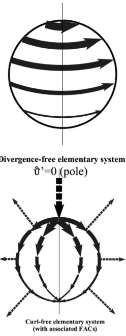
The method of 2D spherical elementary current systems (2D SECS) was introduced by Amm (1997). It is based on two sets of basis functions in spherical coordinates, which can be used to expand any ionospheric surface cur-rent distribution, or any continuously diffecur-rentiable vector field on a sphere. One of the elementary current systems is divergence-free (Jd f,2D), the other one curl-free (Jc f,2D). systems, called scaling factors, and RI is the radius of the ionosphere (Fig. 1).
Associated with the divergence of the curl-free 2D SECS there are field-aligned currents, which are assumed to flow
Fig. 1. The divergence-free 2D SECS and the curl-free 2D SECS with associated FACs.
radially into or out of the ionosphere
j||,2D(r, θ, φ)= sphere at the pole, and a uniform density of FACs flowing out of the ionosphere elsewhere, in such a way that the net flow into and out of the ionosphere is zero. Here, currents are denoted by the symbolI, [I] = A, sheet currents by J, [J] = A/m, and current densities by j, [j] = A/m2.
The magnetic field of the divergence-free 2D SECS was shown by Amm and Viljanen (1999) to have only Br and Bθcomponents both above and below the ionosphere. The magnetic field of the combined curl-free 2D SECS and FACs, on the other hand, is in the φ’ direction and con-fined to the region above the ionosphere for radially flowing FACs (Fukushima, 1976). Thus only the divergence-free 2D SECSs are needed to determine ionospheric equivalent currents.
3.
The 1D SECS Method
In this context, one-dimensionality means independence of the longitude of the chosen coordinate system. 1D vari-ants of the two types of 2D SECSs can be derived by placing poles of infinitely many 2D SECSs of identical amplitude next to each other at a constant latitude
Jd f The unprimed ones, on the other hand, define the coordinate system where the ionospheric currents are to be determined, and as such could have its pole at the geomagnetic or geo-graphic one, for example.
3.1 Divergence-free 1D SECS
Derivation of the divergence-free 1D SECS from Eq. (4) was carried out by Vanham¨akiet al.(2003), and the result-ing current density is given by
Jd f,1D(θ, θ0)=
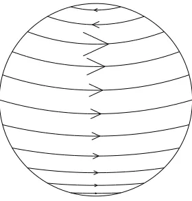
The current density is sketched in Fig. 2.
Theφcomponent of the magnetic field of the system is zero both above and below the ionosphere. The other com-ponents can be written using associated Legendre functions Plm(Arfken and Weber, 1995)
Fig. 2. The divergence-free 1D SECS.
3.2 Curl-free 1D SECS and FACs
Calculation of the curl-free 1D SECS closely follows that of the divergence-free one, the details of which were given by Vanham¨akiet al.(2003). The result is
Jc f,1D(θ, θ0)=
The radial field-aligned currents associated with the curl-free 1D SECS consist again of two parts, FACs flowing uniformly out of the ionosphere, and FACs flowing into the ionosphere atθ =θ0. The current density of the uniform
field-aligned currents at the ionospheric altitude is given by the divergence of the curl-free 1D SECS. The current density of the FACs flowing into the ionosphere atθ =θ0,
on the other hand, is determined by the condition that the net flow into the ionosphere has to vanish. These conditions yield for the FACs
j||,1D(r, θ, φ)=ˆer Magnetic field lines of the combined curl-free 1D SECS and its associated FACs are circles around the z-axis, and therefore Ampere’s law can be applied to calculate their magnetic field. Details of the calculation are given in Ap-pendix A. The result is
B(r, θ, φ)=
3.3 Calculation of ionospheric currents
Measurements of the variation magnetic field compo-nents (Br,Bθ) at locations (ri,θi),i = 1. . .n, can be used to solve the scaling factors I0,d f of the divergence-free 1D SECSs located atθ0,j, j =1. . .m, in such a way that their combined magnetic field as closely as possible fits the mea-sured one. Likewise, the meamea-suredBφcomponent gives the scaling factors I0,c f of the curl-free 1D SECSs. After the scaling factors have been solved, calculating the magnetic field and current density at arbitrary points is a straightfor-ward task.
The problem can be expressed in the matrix form
Br,θ
where the vectorBr,θ contains the measuredr andθ com-ponents of the magnetic field at locations (ri,θi), the vec-torI0,d f scaling factors of the divergence-free 1D SECSs atθ0,j, and the matrixMr,θ the effect of the divergence-free 1D SECSs atθ0,jon therandθcomponents of the magnetic field at (ri,θi). Likewise, the vectorBφ contains measure-ments of the φcomponent of the magnetic field at (ri,θi), vectorI0,c f scaling factors of the curl-free 1D SECSs atθ0,j, and the matrixMφ the effect of the curl-free 1D SECSs at
θ0,jon theφcomponent of the magnetic field at (ri,θi). The scaling factors are obtained by inverting the matrixM
I
The number of measurement points is often smaller than the number of 1D SECSs, causing the problem to be under-determined. Therefore, the matrix inversion has to be per-formed using a suitable technique, for instance the singular value decomposition (SVD, Presset al., 1992).
In SVD, the matrixM ∈Rn×mis decomposed intoM =
U W V T
, whereU ∈ Rn×n andV ∈ Rm×m are orthogonal matrices andW ∈ Rn×m a diagonal matrix. The diagonal elements wkk ≥ 0 of W are called the singular values of M. Ifm > n (underdetermined problem), m−n of the
wkk’s are zero. Among the rest of the singular values, those that are very small compared to the largest wkk represent the unstable part of the solution. The problem is solved by setting 1/wkk = 0, if wkk < ·max(wkk). Here
is an adjustable parameter. The inverse matrix is then M−1=Vdiag(1/wkk)U
T .
In addition to satellite measurements, ground-based mea-surements (cf. Vanham¨akiet al., 2003) can be utilized when determining the divergence-free scaling factors. The curl-free ones, of course, have to be determined solely from measurements above the ionosphere, since the curl-free 1D SECS with FACs does not create a magnetic field below the ionosphere. In addition, due to the assumption of ra-dial FACs, which differ from the more realistic dipole ones, the applicability of the curl-free 1D SECSs was determined by respective tests to be restricted to latitudes higher than approximately 45◦. The 1D assumption breaks down at latitudes higher than approximately 80◦, and therefore the method does not work in this region either. This restric-tion, however, can be circumvented by temporally moving the poles of the 1D SECSs to the equator (see Section 5 for an example). Associated with each curl-free elementary system there is also a certain region, whose magnetic mea-surements cannot be included in determining the amplitude of that particular elementary system. This region, denoted by Fin Fig. 3, is located between the assumed radial FAC sheet of the curl-free 1D SECS and the more realistic dipole one. In this region, magnetic fields of the radial and dipole FAC, which are discontinuous at the FAC sheet, changing their direction, are oppositely directed.
TheF-regions are located at angles
Dipole FAC
Fig. 3. TheF-region between the radial FAC sheet of the curl-free 1D SECS and the more realistic dipole FAC sheet. Magnetic measurements in theFregion cannot be included in determining the amplitude of the concerned curl-free 1D SECS. The width of the region is denoted by θ(r, θ0).
and their width, obtained from the geometry of the dipole field line, is In practise, these regions are left out when determining the curl-free scaling factors by setting the corresponding elements of the matrixMφto zero. This means thatBφat a certain point (r,θ) is given by the combined magnetic field of all other 1D SECSs, except those that have the point (r,θ) located within theirF-region. Or, reversely, the amplitude of the 1D SECS located atθ0is determined using only those
measurement points that do not fall into theF-region of that 1D SECS. An example of the effect of these regions is given in Section 6.
4.
Application Examples—Synthetic Data
Testing of the 1D SECS method was carried out by apply-ing it to two synthetic current density models: a purely one-dimensional electrojet, and a Harang discontinuity model displaying some two-dimensional features.
The starting-point for applying the method to synthetic data was a known ionospheric current density distribution (jr,Jθ,Jφ). The magnetic field of the current distribution was then calculated along a virtual satellite path, and these ‘measured’ magnetic field values were used by the 1D SECS method to first determine the scaling factors and from them to recalculate the magnetic field and current distribu-tion. These were then compared with the original magnetic field and current density to determine the competence of the method. The results of the 1D SECS method were also compared with those of the Olsen method.
4.1 Electrojet
The electrojet was modeled by a gaussian current density distribution
Jφ = −Ae−(θ−θc) 2
2(δθ)2 . (15) In order to determine the other current density components, the geomagnetic field was assumed to beB = −Bˆer, and the convection electric fieldE=Eˆeθ, which gave
⎧
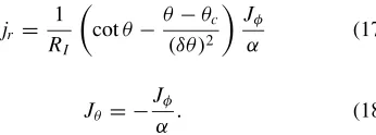
whereP andHare the Pedersen and Hall conductances. It was assumed thatα = H/P = 2 (e.g. Untiedt and Baumjohann, 1993), which then yielded the other two cur-rent density components in the ionosphere in terms ofJφ:
jr =
The magnetic field of the current distribution of the electro-jet along a virtual satellite path at 400 km above the iono-sphere was determined by expanding the current density in 1D SECSs.
In order to recalculate the magnetic field and the current density of the electrojet from the magnetic data, the 1D SECSs were placed 1◦ apart in the ionosphere. The total number of each type of elementary systems for the elec-trojet model then became 36. For the Olsen method, the infinitely long, straight line currents were extended from
θ0= −π . . . πwith a distance corresponding to 1◦between
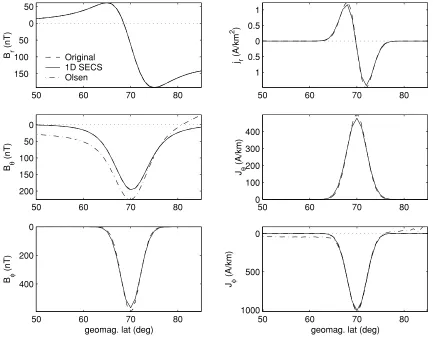
two succesive line currents, and only ther component of the magnetic field was fitted when determing the scaling factors. The results of both methods are given in Fig. 4. Table 1 shows the percentual errors of each fit, defined as
error=
where|B|stands for average of absolute values of the el-ements of the vector. The error of the current density was likewise determined.
For the 1D SECS method, the errors of the fits are very small, and the curves in Fig. 4 are almost indistinguishable from the original ones. The Olsen method is able to repro-duce the electrojet pretty well, but nonetheless the results are not quite as good as those of the 1D SECS method.
50 60 70 80 150
100 50 0 50
B r
(nT)
Original 1D SECS Olsen
50 60 70 80
200 150 100 50 0
B θ
(nT)
50 60 70 80
400 200 0
geomag. lat (deg)
B φ
(nT)
50 60 70 80
1 0.5 0 0.5 1
j r
(A/km
2 )
50 60 70 80
0 100 200 300 400
J θ
(A/km)
50 60 70 80
1000 500 0
geomag. lat (deg)
J φ
(A/km)
Fig. 4. The three components of the magnetic field and current density of the electrojet model as a function of latitude.Jφis determined fromBrand
Bθby the 1D SECS method, and fromBrby the Olsen method. jrandJθare calculated fromBφby the 1D SECS method. Table 1. Percentual errors of the fits of the electrojet model, displayed in Fig. 4, as given by Eq. (19).
Method Br Bθ Bφ jr Jθ Jφ
1D SECS 0.3 0.5 6 8 6 2
Olsen 2·10−4 50 - - - 23
Table 2. Percentual errors of the fits of the electrojet model, displayed in Fig. 5, as given by Eq. (19).
Method Br Bθ Bφ jr Jθ Jφ
1D SECS 0.06 0.05 6 8 6 6
Olsen 0.0012 51 - - - 46
Table 3. Percentual errors of the fits of the Harang discontinuity model, displayed in Fig. 7, as given by Eq. (19).
Method Br Bθ Bφ jr Jθ Jφ
1D SECS 1.3 98 6 72 65 21
Olsen 3·10−4 105 - - - 22
4.2 Harang discontinuity
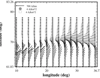
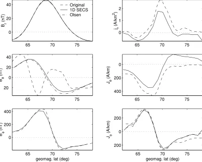
Figure 6 displays the current density of the Harang dis-continuity model, and the path taken by the satellite. The magnetic field of the current distribution was determined using Biot-Savart integration. Figure 7 shows the results of the 1D SECS and Olsen methods applied to the magnetic data of the Harang discontinuity model. The percentual er-rors of the fits are displayed in Table 3.
two-50 60 70 80 40
30 20 10 0
B r
(nT)
Original 1D SECS Olsen
50 60 70 80
30 20 10 0
B θ
(nT)
50 60 70 80
400 300 200 100 0
geomag. lat (deg)
B φ
(nT)
50 60 70 80
1 0.5 0 0.5 1
j r
(A/km
2 )
50 60 70 80
0 100 200 300 400
J θ
(A/km)
50 60 70 80
800 600 400 200 0
geomag. lat (deg)
J φ
(A/km)
Fig. 5. The same as Fig. 4 but with the satellite passing 2000 km above the ionosphere instead of 400 km.
10 20 30 36.77
61.83 70 80 83.26
longitude (deg)
latitude (deg)
700 A/km 4 A/km^2 4 A/km^2
65 70 75 0
20 40
B r
(nT)
Original 1D SECS Olsen
65 70 75 20
0 20 40
B θ
(nT)
65 70 75 0
200 400
geomag. lat (deg)
B φ
(nT)
65 70 75 0
1 2
j r
(A/km
2 )
65 70 75 400
200 0
J θ
(A/km)
65 70 75 200
0 200
geomag. lat (deg)
J φ
(A/km)
Fig. 7. The three components of the magnetic field and current density of the Harang discontinuity as a function of latitude.Jφis determined fromBr
by the 1D SECS method and by the Olsen method. jr andJθare calculated fromBφby the 1D SECS method. The ‘original current density’ is the
current density of the model right below the track of the satellite.
Table 4. Percentual errors of the fits of the CHAMP data, displayed in Fig. 9, as given by Eq. (19).
Method Br Bθ Bφ
1D SECS 6 50 20
Olsen 6 40
-dimensionality of the original current distribution. Even jr andJθfrom the excellentBφfit do not show an overly good resemblance to the original current distribution along the satellite track.
Though the results for the two-dimensional Harang discontinuity are clearly worse than those for the one-dimensional electrojet, the main features of the current den-sity are nonetheless produced pretty well. Performance of both the 1D SECS and Olsen methods appears to be almost equally good.
Further testing with an Omega band model (results not displayed here) revealed that although the performance of the method in a fully two-dimensional case was again worse than with the slightly more one-dimensional Harang discon-tinuity model, even in such a case the method was able to produce the general shape of the current densities.
5.
Application Example—Real Data
In order to test the method with real data, a pass of the CHAMP satellite (Ritteret al., 2004) over the IMAGE
max = 1915 nT
ground equivalent currents, 06Nov2001 05:05:00
60 65 70 800
600 400 200 0 200
B r
(nT)
CHAMP 1D SECS Olsen
60 65 70
1000 500 0 500
B θ
(nT)
60 65 70
1500 1000 500 0 500
geomag. lat (deg)
B φ
(nT)
60 65 70
3 2 1 0 1
j r
(A/km
2 )
60 65 70
0 500 1000
J θ
(A/km)
60 65 70
2000 1000 0 1000
geomag. lat (deg)
J φ
(A/km)
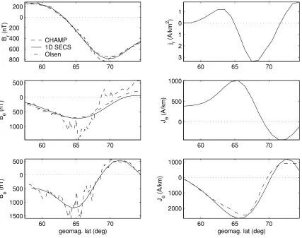
Fig. 9. The three components of the magnetic field and current density measured by the CHAMP satellite on November 6, 2001 at 05:04–05:08 UT, as a function of the geomagnetic dipole latitude. Jφis determined fromBr by the 1D SECS method, and the Olsen method. jrandJθare calculated fromBφby the 1D SECS method.
magnetometer network1 on November 6, 2001 at 05:04–
05:08 UT (8:05–7:26 MLT) was selected. Figure 8 displays a snapshot of the equivalent currents at 05:05 UT. During the overflight, the equivalent current distribution remained pretty much stationary and one-dimensional, as required by the 1D SECS method. When invertingMr,θ using the SVD, we used=0.01 and forMφ,=0.1.
The magnetic field and current density, as given by the 1D SECS method and the Olsen method, are shown in Fig. 9. In a good agreement with the equivalent currents of Fig. 8, both methods display a westward electrojet cen-tered at 65◦geomagnetic latitude. The oppositely directed currents poleward of the electrojet correspond to the less in-tense return flow in the polar cap. At 55◦–65◦and 71◦–75◦ latitudes, the FACs (jr) are mostly directed away from the ionosphere wheras at 65◦–71◦they flow into the ionosphere. In general, due to the distance from the ionosphere, both the 1D SECS method and the Olsen method tend to smooth out the small scale fluctuations present in the magnetic data from the satellite. Jθflows mostly southward on the electro-jet proper between the two main regions of the oppositely directed FACs, with some flow northward at latitudes pole-ward of 70◦. Percentual errors of the magnetic field fits are displayed in Table 4. The ground induced currents, which
1http://www.ava.fmi.fi/image/
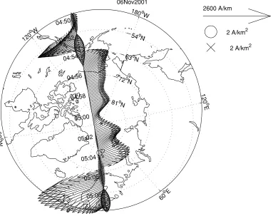
have been ignored in this analysis, affect mainly the am-plitude of Jφ(Olsen, 1996). Finally, Fig. 10 illustrates the application of the 1D SECS method to a polar cap cross-ing. For that purpose, the 1D SECS pole was placed at at 0◦ geographic latitude and 20◦longitude.
6.
Discussion
06Nov2001
120 oW
60
o W
0o
60
oE
120
o
E
180o W
54o N
63o N
72o N
81o N 04:50
04:52
04:54
04:56
04:58
05:00
05:02
05:04
05:06
05:08
2 A/km2
2 A/km2 2600 A/km
Fig. 10. An example of the application of the 1D SECS method to a polar cap crossing. The horizontal ionospheric currents are denoted by the black arrows, the upward FACs by the circles and the downward FACs by the crosses. In order to compute the currents, the 1D SECS pole was placed at 0◦ latitude and 20◦longitude.
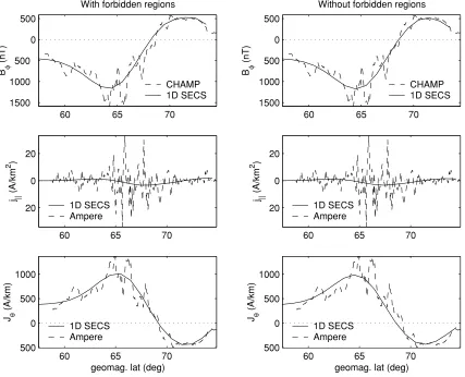
This is due to the fact that the conductive ionosphere causes a damping of the FACs and electric fields of spatial scale smaller than approximately 10–50 km, depending on the ambient conductivities (see e.g. Brekke, 1997, figure 7.35). Hence, if such small scale parts are present in the satellite data, the Ampere’s law-approach is not appropriate to this purpose. In the case of quiet events, however, the results of the 1D SECS method and Eqs. (B.3) and (B.4) often be-come very similar. For comparison, Jθ and j|| calculated using the 1D SECS method and Ampere’s law are shown on the left hand side of Fig. 11.
6.1 Effect of theF-regions
The effect of the F-regions is also demonstrated in Fig. 11. On the right hand side the matrix elements cor-responding to the F-regions (Section 3.3) have not been set to zero when determining the curl-free scaling factors, whereas on the left hand side they have. With the satel-lite flying this low, only approximately 400 km above the Earth’s surface, the effect of not setting the elements to zero is not very significant, as can be seen. Jθ given by the 1D SECS method just appears to have been slightly shifted with respect to the curve derived using Ampere’s law. How-ever, with increasing altitude and decreasing latitude theF -regions get wider and consequently their effects more pro-nounced.
6.2 One-dimensionality
The 1D SECS method assumes one-dimensionality and therefore gives most reliable results when the current dis-tribution under analysis fulfils this condition. To be able
to evalute the quality of the results given by the method, a measure for the one-dimensionality of the situation is needed. One way to achieve this is to use 2D ground-based magnetometer networks, as was illustrated in Section 5. However, these are not always available. Therefore, it is better to be able to do the evaluation relying solely on the magnetic data measured by the satellite. If the divergence-free scaling factors are determined using only ther compo-nent of the magnetic field, the deviation of theθcomponent of the 1D SECSs’ magnetic field from the measured one provides such a measure. The smaller the deviation, the more one-dimensional the current distribution. In a fully 1D case the calculated and measured fields would be equal. In practise, if the shape of the two profiles is approximately the same, the situation appears to be sufficiently 1D. For example, passes of the CHAMP satellite over the IMAGE magnetometer network (like that in Fig. 8) having error of Bθ less than 60% can be considered to be 1D.
7.
Conclusions
60 65 70
Fig. 11. Left: j||andJθcalculated from CHAMP data (November 6, 2001, 05:04–05:08 UT) using both the 1D SECS method and directly applying Ampere’s law.Right:The same as on the left hand side, except that the matrix elements corresponding to theF-regions (Section 3.3) have not been set to zero.
SECSs in the ionosphere can be freely chosen to best ac-comodate the magnetic field measurements. Only the r andθ components of the magnetic field are needed to de-termine the divergence-free horizontal currents, and only the φcomponent to calculate the curl-free horizontal cur-rents and field-aligned curcur-rents. If ground-based measure-ments are available, they can be included in determining the divergence-free scaling factors. In cases that are not fully one-dimensional, the ability of the method to deter-mine the divergence-free currents can be improved by fit-ting just ther component of the magnetic field. The Olsen method, which has commonly been applied to determine ionospheric current from satellite measurements, assumes the geometry to be partly Cartesian, and is only able to produce the part of the horizontal currents perpendicular to the satellite track. The one-dimensionality of the current distribution, and hence the quality of the obtained results can be determined from the difference between the mea-suredBθand that of the 1D SECSs’ when the amplitudes of the divergence-free 1D SECSs have been determined using onlyBr.
Testing of the 1D SECS method was carried out using both synthetic and real data from the CHAMP satellite. The method was established to work excellently in one-dimensional situations, and being able to at least produce the main shape of the currents even if the situation was not
strictly one-dimensional. In 1D cases, performance of the new 1D SECS method appeared to be somewhat better than that of the Olsen method, but in cases which displayed more two-dimensional features, both methods seemed to work almost equally well.
Appendix A.
In this Appendix, calculation of the magnetic field of the combined curl-free 1D SECS and its associated FACs is outlined.
The magnetic field of the combined curl-free 1D SECS and its associated FACs can be determined employing the vector potential this kind of approach does not easily yield a closed expres-sion for the magnetic field, and therefore is merely used to determine the geometry of the field lines. Once the geome-try is known, the magnetic field can be calculated applying Ampere’s law in the integral form.
cur-rent density element and the observation point at (r,θ,φ). Due to symmetry in φdirection, theφ = 0 point can be chosen for the observation point without reducing the gen-erality of the analysis. Figure A.12 displays a sketch of the current system. Elements at (r1,θ1,φ1) and (r1,θ1,−φ1)
have Jx(r1, θ1, φ1) = Jx(r1, θ1,−φ1), Jy(r1, θ1, φ1) =
−Jy(r1, θ1,−φ1), Jz(r1, θ1, φ1) = Jz(r1, θ1,−φ1), and
their distances from the observation point are equal. The sum of their contributions to the vector potential is there-fore a vector with only x and z components. Summing up all the elements pairwise then gives the form of the vector potential at the observation point as A(r, θ,0) =
that is, the magnetic field lines of the combined curl-free 1D SECS and its associated FACs are circles centered on thez-axis:
B(r, θ, φ)=B(r, θ)ˆeφ. (A.4) Ampere’s law can now be employed to calculate the mag-netic field of the system. The law states that a line integral of the magnetic fieldBaround a closed pathC is equal to
μ0times the total current through a surfaceS bordered by
C
Fig. A.12. The curl-free 1D SECS and associated FACs. Magnetic field of the system can be calculated applying Ampere’s law. The concerned surface, bordered by the curveC, is denoted byS. randθdefine the location at which the magnetic field is calculated, andθ0the angle at which the FAC sheet flows into the ionosphere.
θI
Fig. B.13. The geometry for determining Jθ and j|| using Ampere’s law. The circular magnetic field line (the thick, slashed line) passing through the point (r,θ), where the satellite is assumed to lie, borders the funnel-like surface (the thick line), which follows the dipole field and passes through the ionosphere at (RI,θI), closing somewhere below it.
The surface S and curve C are chosen as shown in Fig. A.12. Current passing through the surface S in then solely due to the field-aligned currents, given by Eq. (9). Below the ionosphere (r<RI), current through the surface is zero, but above (r ≥ RI) it is
Performing the integration yields which combined with Eq. (A.4) and
C
B·dl=2πrsinθB(r, θ) (A.8)
then gives the results of Eq. (10).
Appendix B.
In this Appendix, Jθ and associated FACs in dipole ge-ometry are calculated directly without using the curl-free 1D SECSs.
actually any kind of geometry fulfilling the 1D requirement will do just as well. Consequently, Jθ and FACs can be calculated directly using Ampere’s law. Figure B.13 shows the respective geometry for FACs flowing along dipole field lines. The circular magnetic field line passing through the point (r,θ) borders the funnel-like surface, which fol-lows the dipole field and passes through the ionosphere at (RI,θI), closing somewhere below it. Only Jθ contributes to the total current passing through the surface. Therefore, according to Ampere’s law,
2πrsinθBφ(r, θ)= −μ02πRIsinθIJθ(RI, θI), (B.1) where the angleθI is given by
θI =sin−1
RI r sinθ
. (B.2)
Jθcan now be solved from Eqs (B.1) and (B.2)
Jθ(RI, θI)= −
r RI
3/2
Bφ(r, θ)
μ0
(B.3)
and the FACs are given by the current continuity
j||(RI, θI)= − 1 rsinθ
∂
∂θ(sinθJθ). (B.4)
These results equal those of the 1D SECS -approach in the case when infinitely many curl-free 1D SECSs are placed in the ionosphere, apart from the geometry of the FACs.
Acknowledgments. The authors wish to thank Dr. Patricia Rit-ter from GFZ Potsdam for providing the CHAMP satellite data, and Dr. Nils Olsen from Danish Space Research Institute for his valuable advice concerning the application of his method. The two referees are acknowledged for their comments, which greatly improved the outcome.
References
Amm, O., Ionospheric elementary current systems in spherical coordinates and their application,J. Geomag. Geoelectr.,49, 947–955, 1997. Amm, O. and A. Viljanen, Ionospheric disturbance magnetic field
continu-ation from the ground to ionosphere using spherical elementary current systems,Earth Planets Space,51, 431–440, 1999.
Arfken, G. and H. Weber,Mathematical Methods for Physicists, Academic Press, 4th ed., 1995.
Brekke, A.,Physics of the Upper Polar Atmosphere, John Wiley & Sons Ltd, 1997.
Fukushima, N., Generalized theorem for no ground magnetic effect of vertical currents connected with Pedersen currents in the uniform-conductivity ionosphere, Rep. Ionos. Space. Res. Japan, 30, 35–40, 1976.
Olsen, N., A new tool for determining ionospheric currents from magnetic satellite data,Geophys. Res. Lett.,23, 3635–3638, 1996.
Press, W. H., B. P. Flannery, S. A. Teukolsky, and W. T. Vetterling, Numer-ical Recipes, 2nd ed., 973 pp., Cambridge University Press, Cambridge, 1992.
Pulkkinen, A., O. Amm, A. Viljanen, and BEAR Working Group, Iono-spheric equivalent current distributions determined with the method of spherical elementary current systems,J. Geophys. Res.,108, 1053, 2003.
Ritter, P., H. L¨uhr, A. Viljanen, O. Amm, A. Pulkkinen, and I. Sillanp¨a¨a, Ionospheric currents estimated simultaneously from CHAMP satellite and IMAGE ground based magnetic field measurements: a statistical study at auroral latitudes,Ann. Geophys.,22, 417–430, 2004. Untiedt, J. and W. Baumjohann, Studies of polar current systems using the
IMS Scandinavian magnetometer array,Space Sci. Rev.,63, 245–390, 1993.
Vanham¨aki, H., O. Amm, and A. Viljanen, 1-Dimensional upward contin-uation of the ground magnetic field disturbance using spherical elemen-tary current systems,Earth Planets Space,55, 613–625, 2003. Viljanen, A., A. Pulkkinen, O. Amm, R. Pirjola, T. Korja, and BEAR
Working Group, Fast computation of the geoelectric field using the method of elementary current systems and planar earth models,Ann. Geophys.,22, 101–113, 2004.