A two-stage GIS-based optimization model for the dry port
location problem: A case study of Iran
Mehran Abbasi1, Mir Saman Pishvaee1* 1
School of Industrial Engineering, Iran University of Science and Technology, Tehran, Iran [email protected], [email protected]
Abstract
This article aims to investigate the location of dry ports by providing a two-stage GIS-optimization model. At the first stage, the appropriate points for establishing dry ports were identified using GIS and hierarchical analysis process; then, the suitable points were introduced as the potential points to the second stage model. At the second stage, by providing a multi-objective integer model, the location of the port and the transportation modes used to transship the goods from/to the dry port are investigated. Finally, the model is linearized using a heuristic method and, then, is developed using its robust counterpart in order to deal with the uncertainty in the model parameters. To investigate the performance of the model, the problem was solved using GAMS software for the case study of Iran. The obtained numerical results indicated that the use of the developed model and establishment of the dry port led to the reduced costs, reduced variable environmental effects of the seaport, improved accountability to the customers of these ports, and consequently increased
competitiveness.
Keywords: Dry port, multi-modal transportation, geographic information system (GIS), robust optimization, logistics planning
1- Introduction
Over the years, the development in the use of containers in international transportation has been completely obvious so that seaport-dependent transportation rate in Europe has been increased by 100% during the first 10 years in the onset of the 21st century (Commission, 2000). Thus, such increased transportation has caused major problems in seaports. Lack of sufficient space, high volume, and density of tasks such as unloading, loading, customs, as well as sending and receiving commodities are some of these problems (Jaržemskis and Vasiliauskas, 2007). The increased flow of containers was modeled and simulated by Parola and Sciomachen (2005), the results of which showed the significant congestion and increase in the road traffic around seaports and even at farther distances. On the other hand, environmental problems have been increased in the past decade and, thus, the logistics systems play a significant role in reducing such effects (Aronsson and Huge Brodin, 2006). Dry ports are the example of the measures taken to resolve these problems (Dadvar et al., 2011).
Dry ports are located in the internal parts of the country compared to the seaports, but are directly related to seaports. Furthermore, in the international transportation of commodities, they are correlated with the destinations of imported commodities as well as departures of exported commodities.
*Corresponding Author
ISSN: 1735-8272, Copyright c 2018 JISE. All rights reserved
Journal of Industrial and Systems Engineering
Vol. 11, No. 1, pp. 50-73
Dry ports are applied in the coastal as well as landlocked countries; however, in all of them, land transportation methods provide easy access to seaports (UNCTAD, 1991). These inner terminals, as the development of seaports, have led to their increased capacity and efficiency as well as reduced road traffic by transferring traffic to railways or inland waters (Do et al., 2011). Furthermore, dry ports can be also considered as one of the logistics system strategies for reducing environmental problems (Roso, 2007). Regarding the above-mentioned advantages, these ports are considered as one of the major role-players in the water transportation chain (Woxenius et al., 2004).
The concept of the dry port was first introduced by Munford (1980) in 1980, in which it was considered as the case study of Argentina and the term “dry port” was used specifically.
With regard to the advantages of dry ports, this field has been highly regarded in the literature in recent years. Apropos of dry ports, studies have been mostly focused on the concepts (Veenstra et al., 2012, Roso et al., 2009, Roso, 2007), creation and development (Beresford et al., 2012), implementation and execution (González-Sánchez et al., 2015, Kovacs et al., 2008), and policy (Haralambides and Gujar, 2011, Ng and Gujar, 2009). Also, three review articles by Cullinane et al. (2012), Roso and Lumsden (2010), and Beresford et al. (2012) have investigated the literature in this regard; on the other hand, only a few works have been focused on the location of dry ports using mathematical modeling; thus, further research is required.
Presenting a mathematical model for the concept of dry ports was initiated by Zeng et al. (2011) through proposing a mixed integer programming (MIP) model for their location. In this article, the relationship between three main components of the network, namely customer, dry port, and seaport, was taken into consideration completely whether in terms of sending and receiving the commodities or presence of a relationship between the components. One of the considerable points in this model was that the relationship between the dry ports and seaports and the relationship between the seaports or dry ports and customers were assumed using the railways and roads, respectively.
In the proposed models in this field, due to the enlargement of the model at the time of implementation, the heuristic and meta-heuristic methods are often used (Zeng et al., 2011, Feng et al., 2013, Qiu and Lam, 2014, Qiu et al., 2015, Chang et al., 2015); in few cases (Ambrosino and Sciomachen, 2014, Crainic et al., 2015), the exact solution methods are applied. Subsequent to the aforementioned article, by adding the maintenance and repair costs of the communication routes, in addition to considering the transportation cost and, of course, disregarding type of transportation, Feng et al. (2013) presented a nonlinear model and solved it using the genetic algorithm (GA).
An example of the classifications of the presented models is to consider a variety of transportation methods or to consider them as the same, while each of these methods might have the shipping capacity. As a combined classification, in the most complicated mode, a multi-modal transportation has capacity (e.g. (Ambrosino and Sciomachen, 2014)) and, in the simplest mode, transportation has a shipping method and lacks capacity (e.g. (Feng et al., 2013, Qiu and Lam, 2014, Qiu et al., 2015)). In the article by Ambrosino and Sciomachen (2014), despite the use of multi-modal transportation mode with capacity, the model was written as linear and solved precisely and easily by the software, the results of which were analyzed for Genoa.
The articles presenting mathematical models on dry ports have been fully focused on the location issue and only two articles by Qiu and Lam (2014) and Qiu et al. (2015) have investigated the issues of inventory maintenance and storage costs. In the articles by Qiu and Lam (2014), inventory and transportation costs were taken into account, and the profit rate, number of shipped containers, and commodity storage cost were expressed as the output of the model. Moreover, in a similar article by Qiu et al. (2015), the inventory pricing was
investigated. In this article, in contrast to the previous one (Qiu and Lam, 2014) stating the issue of transferring from the seaport to the dry port and eventually to the customer, the transportation from the customer to the dry port and, then, to the seaport was taken into consideration.
As previously mentioned, except for the two articles investigating the subject of pricing, other articles have presented models for the location. For example, Chang et al. (2015) presented a two-step model for the location. In this model, first, using the decision-making techniques, the candidate points for establishing the dry port were extracted; then, by providing a location model, the optimal points for establishing the port were specified. Besides, in this model, the multi-modal transport can be seen. The last article used the mathematical optimization model on dry ports was by Crainic et al. (2015) in which the transport rate was considered as the model outcome and, despite adding time to the model causing its complexity at the time of solution, the model was solved accurately.
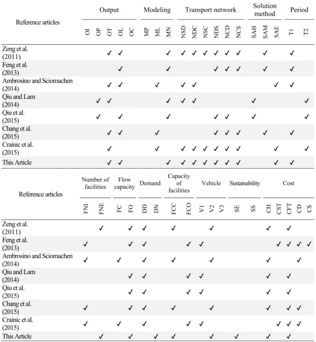
Table 1. Encoding various problems in the field of dry ports
Classification Code Classification Code
Out
put
Inventory OI
Pro bl em defi nition Num ber o f facili
ties Endogenous FNI
Storage price OP Exogenous FNE
Transportation rate OT
Flow capac
it
y Flow with capacity FC
Location and allocation OL Flow without capacity FO
Capacity of facilities OC
De
man
d Deterministic DD
Modeling
Mixed random integer programming MP Non-deterministic DN
Mixed integer linear programming ML
Capa cit y of facilitie s
With capacity FCC
Mixed integer nonlinear programming MN Without capacity FCO
T rans port net w ork Sen din
g to
cust
omer
From seaport to dry port NSD
Ve
hi
cle One type V1
From dry port to customer NDC Two types V2
From seaport to customer NSC Multiple types V3
Receiving from
cu
stom
er
From dry port to seaport NDS
Su
stai
nability
Environment SE
From customer to dry port NCD
Social SS
From customer to seaport NCS
So
luti
on
met
hod
Heuristic SAH
Cost
Maintenance in dry port CH
Meta-heuristic SAM Transportation constant CST
Exact SAE Transportation variable CFT
Period
Single-period T1 Dry port operation CD
As seen in tables 1 and 2, the articles on dry ports have presented models based on various features. To define the location model of dry ports, it is primarily necessary to specify the appropriate potential points for establishing these ports. In the relevant literature, the potential points are determined by experts and, then, inserted in the model as parameters; however, identification of these points depends on the factors such as land slope, proximity to roads and railways, and type of land use; all of these factors should be taken into account. On the other hand, in the literature of other fields, most of the aforementioned instances are combined as 0 and 1, while these factors are not necessarily the same in terms of importance. One of the useful instruments, the use of which has been significantly expanded, is remote measurement and geographical information systems (GIS). Geographical information systems play a key role by considering the roads and other geographical features to find the locations of facilities (Church, 2002). In addition, GIS contribute significantly to collect, classify, combine, and analyze the geographical data for location and optimization in the transportation network (Alçada-Almeida et al., 2009) and are also used for data handling and result analysis (Teixeira et al., 2007). The Combination of decision making analysis model and geographical information systems cause to emerge the interesting research fields (Wang et al., 2004). The use of GIS facilitates the identification of qualitative and quantitative variables, measurement of the parameters affecting these variables, interpretation of their relationship (Malczewski, 2004), and finally identification of the appropriate regions for establishing dry ports. By these instruments for each of the factors affecting the selection of the potential points, the geographical layers are defined; then, regarding the importance of the layers and using the AHP technique, the layers are merged and, finally, the appropriate potential points are obtained to be presented to the mathematical model (Mohseni et al., 2016).
Table 2. Investigating the research gap in the literature Period Solution method Transport network Modeling Output Reference articles T2 T1 SA E SAM SAH NCS NC D ND S NSC ND C NSD MN ML MP OC OL OT OP OI ✔ ✔ ✔ ✔ ✔ ✔ ✔ ✔ ✔ ✔ ✔ Zeng et al.
(2011) ✔ ✔ ✔ ✔ ✔ ✔ ✔ Feng et al.
(2013) ✔ ✔ ✔ ✔ ✔ ✔ ✔ Ambrosino and Sciomachen
(2014) ✔ ✔ ✔ ✔ ✔ ✔ ✔ Qiu and Lam
(2014) ✔ ✔ ✔ ✔ ✔ ✔ ✔ Qiu et al.
(2015) ✔ ✔ ✔ ✔ ✔ ✔ ✔ ✔ Chang et al.
(2015) ✔ ✔ ✔ ✔ ✔ ✔ ✔ ✔ ✔ ✔ Crainic et al.
(2015) ✔ ✔ ✔ ✔ ✔ ✔ ✔ ✔ ✔ ✔ ✔ This Article Cost Sustainability Vehicle Capacity of facilities Demand Flow capacity Number of facilities Reference articles CS CD CFT CST CH SS SE V3 V2 V1 FCO FCC DN DD FO FC FNE FN I ✔ ✔ ✔ ✔ ✔ ✔ ✔
Zeng et al. (2011) ✔ ✔ ✔ ✔ ✔ ✔ ✔ ✔ ✔
Feng et al. (2013) ✔ ✔ ✔ ✔ ✔ ✔ ✔ Ambrosino and Sciomachen (2014) ✔ ✔ ✔ ✔ ✔ ✔ Qiu and Lam
(2014) ✔ ✔ ✔ ✔ ✔ ✔ Qiu et al.
(2015) ✔ ✔ ✔ ✔ ✔ ✔ ✔ ✔
Chang et al. (2015) ✔ ✔ ✔ ✔ ✔ ✔ ✔ ✔
Crainic et al. (2015) ✔ ✔ ✔ ✔ ✔ ✔ ✔ ✔ This Article
Another issue that has not been considered in any of the articles is the environment. In the current era, due to the consumption of fossil fuels and airborne waves, freight transport has significant effects on the environment (Wang et al., 2015); therefore, the use of objective functions that take into account the environment can reveal the importance of dry ports more than ever. One of the reasons for the use of such objective functions is the environmental effects of transportation activities (Zachariadis et al., 2015). Iran is among the countries encountering numerous problems in terms of air pollution, especially in recent years, and this environmental problem has troubled the Iranian people. Therefore, it is essential to consider this problem in most of the activities and plans of the private, and particularly governmental, institutions. The use of some types of transportation vehicles might lead to reduced costs, but reducing environmental pollutions is of greater importance for the Iranian government. Accordingly, regarding the importance of this subject in Iran, besides investigating the location for
establishing a dry port, the present article attempted to consider the issue of environment in the presented model. Consequently, a mathematical multi-objective location model was written to solve this problem.
The rest of this article is organized as follows: first, a brief description of the problem is expressed in Section 2; then, in Section 3, the mathematical model and its required tools are presented. In Section 4, the mathematical model and GIS are implemented with the information on the case study of Iran. Then, the numerical results are analyzed and evaluated. Finally in Section 5, the conclusion is presented.
2- Problem Definition
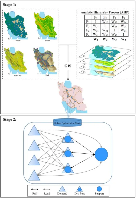
A dry port is typically founded to reduce the volume of seaport-related activities. In order to establish dry ports, first, appropriate places should be identified and, then, the optimal points should be determined from among them. Identifying the appropriate locations or potential points depends on various factors including land slope, proximity to roads and rail routes (Chang et al., 2015), and land use. Furthermore, choosing the optimal points is carried out based on several indices, including transportation cost, the operational cost of dry ports, etc. In the related literature, the potential points are determined by the experts and, then, inserted in the model as parameters since avoiding the investigation of the aforementioned geographical factors would lead to the increased error in experts’ decisions. On the other hand, in the literature, the aforementioned instances are often combined as 0 and 1, while they are not necessarily the same in terms of importance; superiority of each of them to others should be determined by the experts because it is not sufficient to have all the factors for a single point of the investigated area; thus, they should be determined based on their degrees of importance since the factors are quite compensatory for each other. All the selected points should have a minimum level of all the factors; however, the points that have this minimum level should be determined with regard to the importance of the criteria relative to each other as well as the score obtained by each point in a criterion. Therefore, the present article tried to solve this problem using a two-stage model according to figure 1:
Stage 1: In this stage, at first the effective geographic factors on choosing the suitable location to establish the dry port are identified. Then regarding expert opinions and using analytic hierarchy process (AHP) method, the numerical weight of factors is derived by comparing them to each other. Afterwards, the geographic layer of these factors are created in the GIS software environment and with respect to the weights derived from AHP method, the created layers merged into a final layer. Finally, the suitable points to build the dry port are extracted and introduced to a mathematical model in the second stage as the potential points.
Stage 2: A mathematical model is developed at this stage based on features of dry port transportation network for the location of the ports. This model evaluates and analyzes the features of the potential points derived from the previous stage and considered as the input points for this stage, stand on environmental effects and costs involved. Finally, the model determines the ideal locations for establishing the dry ports.
Developing the mathematical location model in the second stage is based on that the dry ports are commonly connected to the seaports through railways. Sending or receiving the goods from the customer to the seaport or vice versa can be carried out through the dry port or directly by the seaport (Roso and Lumsden, 2009), meaning that as shown in figure 1, there are two ways for sending (receiving) the marine cargo to (from) the customer: (1) Sending directly from the seaport to the customer by road transportation, or (2) transferring to the dry port through railway and delivering to the customer by road transportation, which is closer to the reality considering the combined transportation (road and rail) because, in many cases and also in the case investigated in this article, after receiving the cargo from the dry port, transportation is carried out through the roads.
Fig. 1. Schematic of two-stage location model of dry ports
Due to the budget constraints and regarding the opinions of the relevant authorities, it is necessary to establish a certain number of dry ports. In order to choose some of these locations, two objectives should be examined: the first objective is to minimize the total cost which includes the costs of transportation between each of the network components of the network; besides, there is a specific operational cost for dry ports in accordance with the chosen location. The second objective is to minimize the environmental pollution, which has not been discussed in any of the articles in this regard; however, it is of great importance due to the growing increase of the pollutants. Among the other features causing the complexity of this problem is
the multi-modal transportation because the issues of multi-modal transportation and dry ports have been such tied together that Leveque and Roso (2002) called dry ports as the multi-modal terminal.
In order to get the model closer to the reality, the capacity of dry ports is assumed limited and, thus, it is impossible to send the goods to these ports beyond their capacity; therefore, in case of the lack of capacity in any of the dry ports, the goods will be inevitably sent directly from the seaport to the customer through road transportation. Considering the problems of the international trade and, as a result, fluctuations of the trade inside the country and also regarding the political and macroeconomic problems and, finally, due to the uncertainty of the dry port demand rate, it is highly important and practical to consider the uncertainty and plan for it, which would result in the proactive measures and actions.
3- Model formulation
As previously mentioned, for the location of the dry ports, a two-stage model was proposed in this article. At the first stage, the suitable points for establishing the dry ports are specified; then, at the second stage, these points are introduced as the potential points into the mathematical optimization model and, eventually, the final location for establishing the dry port is determined.
In order to determine the suitable points, first, the indices and sub-indices affecting the establishment of the dry port are identified; on this basis, in the case study of the present article, the land slope, proximity to the roads and railways, and land use are determined as the indices. After identifying these factors, the corresponding geographic layers are formed using ArcGIS software; then, in order to merge these layers, commonly two methods, namely Boolean and weighted overlay, are normally used (Malczewski, 1999). The Boolean method is considered in the cases in which the factors are non-compensatory so that if all the factors are essential, the operator “and” will be used, and if one of the factors is sufficient for determining the points, the operator “or” will be used (Gorsevski et al., 2012). However, when the factors are compensatory and not necessarily of the same importance, the weighted overlay method will be used, as in the present study. In this method, one of the favorable approaches for determining the weights of geographic layers is the AHP method (Şener et al., 2010). In this regard, in order to determine the importance and weight of the indices and sub-indices relative to each other, first, their paired comparison is made by the experts and, then, the importance of the weight of each of the identified factors relative to each other is extracted using the AHP method. After determining the weights, using ArcGIS software and output weights of the AHP method, the developed geographical layers are merged; finally, after merging the layers, the suitable points for establishing the dry port are identified and given to the deterministic and robust mathematical model as the potential points.
3-1- Deterministicmodel
In this section, a mathematical multi-objective mixed integer programming model is presented, the first objective of which is to minimize the total costs and the other one is to minimize the environmental effects. Thus, first the sets, parameters, and variables are introduced:
Sets:
I Set of all the nodes of the network in land iI
J Set of all the potential points for establishing the dry port jJ Parameters:
Total transported goods at node i in a non-deterministic manner (the goods exported from and imported to the node)
d1
i,j Road distance between i and j d1
i0 Road distance between i andseaport d2
i,j Rail distance between i and j d2
j0 Rail distance between j and seaport
C1 Road transportation cost unit per traveled distance C2 Rail transportation cost unit per traveled distance
C3 Operational cost unit of dry port per amount of goods at the port
V1 Coefficient of pollutant production by road transportation per traveled distance and
transported cargo
V2 Coefficient of pollutant production by rail transportation per traveled distance and
transported cargo
P Determined number of dry ports to be established Qj The Capacity of dry port j
Decision variables:
yj 0 and 1 variables of choosing the dry port location so that if the potential location is
selected, it will be equal to 1; otherwise, 0
Wij 0 and 1 variables of connecting the dry port to other nodes so that if the dry port j is
connected to node i, it will be equal to1;otherwise, 0 Xa
i Goods transported from (to) customers to (from) the seaport through the dry port Xb
i Goods transported from (to) customers to (from) the seaport directly through the roads
1 2 1
1 1 0 2 3 0 1
a a
j
a b
ij i ij ij i j ij i i i
i i
Min Z
W X d C W X d C W X C
X d C (1)1 2 1
2 1 0 2 0 1
a a b
i ij ij i ij j i i
i i
j
Min Z
X W d V X W d V
X d V (2)1 j
ij
W i
(3)j j
y P
(4),
ij j
W y i j (5)
a b
i i i
X X O i (6)
j a ij i i
W X Q j
(7)
, 0,1 ,
j ij
y W i j (8)
, 0
a b
i i
X X i (9)
In equation (1), the first objective function seeks to minimize the costs of road transpiration between the seaport and customer and between the dry port and customer, the costs of rail transportation between the dry port and seaport, as well as the operational costs of the dry port. In the dry port transportation network, the amount of CO2 emission depends on the type of transportation mode and also the distance between customers, dry ports, and sea ports. In this regard, the second objective function presented in equation (2) minimize the CO2 emission which has a bad effect on the environment.
The first constraint (3) indicates that each customer can receive the services only from one dry port. Constraint (4) states the total number of the dry ports that should be established because the determination of the number of dry ports has been assumed as exogenous in the problem. The relationship between variables Wij and yj is mentioned in equation (5), stating that
there will be a relationship between the customer i and dry port j if the dry port is established and exists at node k. Equation (6) shows that the total goods received (sent) by the customer
through road, and rail transportation is equal to the customer’s demand and the customer’s demand is responded to completely; of course, the customer’s demand has had deep uncertainty, the insertion of which in the model was discussed in the “solution description” section. Constraint (7) indicates that the capacity of each dry port is observed in order to prevent the total sent goods from exceeding its capacity. Moreover, Equations (8) and (9) determine the type of the decision variables.
3-2- Linearization method
With regard to the non-linearity of the model, a heuristic method expressed in the relevant literature was used to linearize it. In this method, by adding the variable, the non-linear model is converted into a linear one. This method is used when both decision variables are multiplied and leads to the non-linearity of the model so that if one of the variables is 0 and 1, the model will become linear by defining and substituting a new variable instead of the multiplication of the aforementioned two variables (Jaberi and Rafeh, 2014). Thus, in order to linearize the term “A*B”, if A is a 0 and 1 variable and B is a positive continuous variable, then continuous variable C will be defined and assumed as equal to the aforementioned terms (C=A*B). After defining variable C, the following constraints are added (up representing the upper limit of variable B and low representing the lower limit of variable A) (Chen, Baston, and Dang 2010):
(10)
∗ ∗ 0
3-3-Robust optimization
Uncertainty plays a significant role in the international trade models and in the global supply chain design (Garivani and Pishvaee, 2017). For example, the demand parameter used in the mathematical model depends on the political, social, and particularly macroeconomic factors of a country. For instance, in Iran (the case study of the present article), the presence or absence of economic sanctions, due to the political issues, plays a significant role in the trade fluctuations of the country; on the other hand, the uncertainty in the international trade volume has caused some problems in this regard. For example, the trade volume in Japan was decreased due to the economic recession by 50% from September 2008 to February 2009 (Novy and Taylor, 2014) and resulted in a big shock in the trade of this country; furthermore, the uncertainty also affected the import and export rates (Wolf, 1995). Moreover, since the dry ports are regarded as a part of import and export network along with the seaports, uncertainty in the international trade would affect the demand of the dry ports.
One of the methods that have been recently considered by researchers for dealing with uncertainty is the robust optimization method. This method, in the case of the presence of uncertainty in the parameters of the problem, would help decision-makers act with respect to its risk-taking and risk-aversion levels. Finally, the use of this approach would result in the solutions with less sensitivity to the uncertainty; besides, this method seeks to find solutions that remain robust and feasible in the case of emerging uncertainty. The use of this approach in the strategic decisions of the dry port would lead to the decisions with less sensitivity to the non-deterministic parameters.
This approach was presented by Soyster (1973) in 1973. Although the term “robust optimization” is not used in the present article, it is supposed that the parameters with uncertainty change in an interval and, thus, a model is provided to produce a feasible solution in the worst case. However, in most cases, it would be less likely that all of these parameters are in their worst status; instead, they impose very high costs on the model. In order to resolve this problem, Ben-Tal and Nemirovski (2000) and El Ghaoui et al. (1998) have presented models under the elliptical uncertainty set. Although in these two models, the conservativeness level of Soyster’s model is reduced, the basic linear model is turned to a non-linear one. Furthermore, Li et al. (2011) showed that the models presented based on the rhombic and square uncertainty set as well as their combination would maintain the linearity of the initial problem, but other sets would lead to the nonlinearity of the model.
In 2004, Bertsimas and Sim (2004) presented a model that, in addition to maintaining the linearity of the initial problem, completely controlled the model’s conservativeness level by considering the uncertainty budget. The use of this robust optimization model in this article made it possible to investigate and make strategic decisions of the dry port for different conservative levels (uncertainty budget).
In this method, a budget parameter Γ ∈ 0, | | was introduced to control the conservativeness level of the solution so that | | indicates the number of the non-deterministic factors in the ith constraint and Γ adjusts the robustness level versus conservativeness of the solution and is called the uncertainty budget for constraint i. If Γ 0, the effect of the changes in the coefficients will be ignored; on the other hand, if Γ | |, then all the possible changes in the coefficients will be taken into account, which is the most conservative state. Moreover, if Γ ∈ 0, | | , the decision-maker decides on the level of changes to be applied. In order to describe this structure, the following model is considered:
(11)
. . ∀
∈
where indicates the actual values for the coefficients’ parameters that are put in the range of , . Also, and indicate the nominal values and the range of fluctuations, respectively. In the ith constraint, it is improbable for all parameters of the
non-deterministic factors to take the worst state at the same time; thus, this formulation is aimed to control the Γ number of those parameters that take the values of the worst state.
max
∪ | ⊆ ,| | , ∈ \ Γ Γ
∈
∀ (12)
where indicates a subset containing Γ non-deterministic parameters in the constraint and is an index for describing the non-deterministic parameter when Γ is not an integer; thus, the above constraint expresses that the worst values can be selected as much as the Γ number of the non-deterministic parameters at the same time. It is clear that when Γ selects an integer
Γ Γ , then the constraint will be changed as follows:
max | ⊆ ,| |
∈
when Γ is not an integer, the non-deterministic parameter can be changed up to
Γ Γ , while the protection function , Γ is defined as follows:
, Γ max
∪ | ⊆ ,| | , ∈ \ Γ Γ
∈
(14)
In this case, , Γ is equal to the objective of the following model so that the optimal solution ∗ contains Γ variables in 1 and one variable in Γ Γ .
∗ ∈
(15) . .
∈
Γ 0 1 ∀ , ∈
After writing the dual problem, we will have: Γ
∈
(16) . . ∗ ∀ , ∈
0 ∀ ∈ 0 ∀
where corresponds to the dual variable of the inequality 1 and corresponds the dual variable of the inequality ∑ ∈ Γ. Finally, after substituting the above model in the initial problem, the following robust model will be obtained:
(17) . . Γ
∈
∀ ∗ ∀ , ∈
0 ∀ ∈ 0 ∀
In this model, budget parameter Γ determines the number of coefficients that can take the worst values for any constraint at the same time and the robust optimization model remains linear. This is different from the formulation of the worst case, in which all the given parameters take the worst values at the same time without controlling the conservativeness level of the solution.
In order to solve and deal with the multi-objective problems, numerous methods have been proposed in the literature. Choosing an appropriate method for a particular application is not simply possible because each one has its own specific advantages and disadvantages (Ehrgott et al., 2016). On the other hand, according to Ignizio (1983), the term “best” cannot be used for a single method for all the problems. In the present paper, the idealistic programming method was used because of being a flexible and relatively simple method that facilitates investigating different scenarios. The idea of the idealistic programming is such that an ideal is determined for each objective and the model seeks for a solution that is closer to the objectives as much as possible (Charnes et al., 1955). Moreover, in the present article, from among various approaches to the idealistic programming expressed in the literature, the weighted goal programming method was used because the objectives were compensatory for each other with
different levels of importance so that the importance of the ideal k was considered with weight Rk.
Hence, the following variables and parameters were added to the model: Parameters:
Rk Weight of importance of the kth objective function Gk Idealof the kth objective function
M A very large number Decision variables:
f –
k Negative deviation from the kth objective function f +
k Positive deviation from the kth objective function Sij Alternative variable for linearization
Considering the presented explanations and the equality a
ij ij i
S W X (for linearization) for each i and each j and also assuming OiOiO Oˆi, iOˆi (for the robust model), the model was finally rewritten as follows:
1 1 2 2
Min Z R f R f (18)
1 2 1
1 2 3 1 1 1 1
b
ij ij ij jD ij i iD
i
j i
S d C S d C S C X d C f f G
(19)1 2 1
1 2 b 1 2 2 2
ij ij ij jD i iD
i
j i
S d V S d V X d V f f G
(20)1 j
ij
W i
(21)j j
y P
(22),
ij j
W y i j (23)
a b
i i i i i i
X X M O i (24)
ˆ
i Mi Oi i
(25)
j ij i
S Q j
(26), a
ij i
S X i j (27)
. ,
ij ij
S M W i j (28)
. a ,
ij ij i
S M W X M i j (29)
, 0,1 ,
j ij
y W i j (30)
, , ,
, i i 0
a b
i i ij
X X S M i (31)
After integrating and linearizing the model, it was solved using the software, the results of which were obtained in accordance with the case study of Iran.
4- Case study and numerical results
Having more than 5800 kilometers of coastline, including the islands, Iran has a great potential for marine transportation; besides, the strategic situation of the country in terms of the commodities transit indicates the significant role of the naval fleet in the development of the country’s transportation. Iran, as the crossroad of the world trade, is located in the course of north-east, east-west, and central trade corridors in Asia; therefore, while being at the heart
of the trade corridors, it can play a special role in providing services based on the transit of commodities from Asia to Europe as well as the countries around the Persian Gulf and the central Asian countries. Such an appropriate opportunity has motivated policymakers to consider the issue of transit as an alternative for the incomes derived from the oil reservoirs.
However, the wide geographical area of Iran and long distance between the cities and coastal ports have caused numerous problems for exporters, importers, as well as transit of goods. Besides, the high costs of road transportation would lead to the increased final price of the domestic products, which reduces the competitive power of the domestic producers compared with the foreign ones. In this regard, the use of the hub logistical technique and, specifically, the dry ports can be effective and useful.
Regarding the geographical area, first, the suitable points for establishing dry ports should be selected; for this purpose, the following factors were examined:
Proximity to roads and railways: In the literature of dry ports, these ports have been called
multimodal terminals (Ng et al., 2013) so that the goods are commonly entered into these ports using a transportation method and exit through another method. Furthermore, similar to the present article, in most cases, seaports and dry ports are connected through a railway and, subsequently, a road. Thus, proximity to roads and railways is of great importance because long distances would result in very high costs for road construction and connecting dry ports to the road network of the country. For this purpose, multiple buffers were used and, after performing the raster with the precision of 1 km as separate layers, proximity to the roads and railways was taken into account in the model.
Land slope: For the economic construction of dry ports and with regard to the presence of
the equipment required for changing transportation method from roads to railways, the establishment of these ports requires lands free of the steep slope. To reduce the costs, investigation of the appropriate locations was limited to the lands with the slope of fewer than 5 degrees. In order to create the land slope layer in Iran, the digital elevation model, as well as the command “surface” in ArcGIS software, was used.
Land use: Considering the environmental issues and other features of dry ports, including
reduction of traffic, it is better to construct these ports at places with fewer problems in terms of land use. One of the functions of dry ports is to remove containers from the port city and help reduce traffic in cities; thus, establishing these ports in urban lands cannot be reasonably justified. Moreover, the wood/forest lands are not suitable for this purpose, while barren lands and desert areas are considered as the appropriate cases. The land use map was received from Iran National Cartographic Center (NCC) and rasterized with the precision of 1 km.
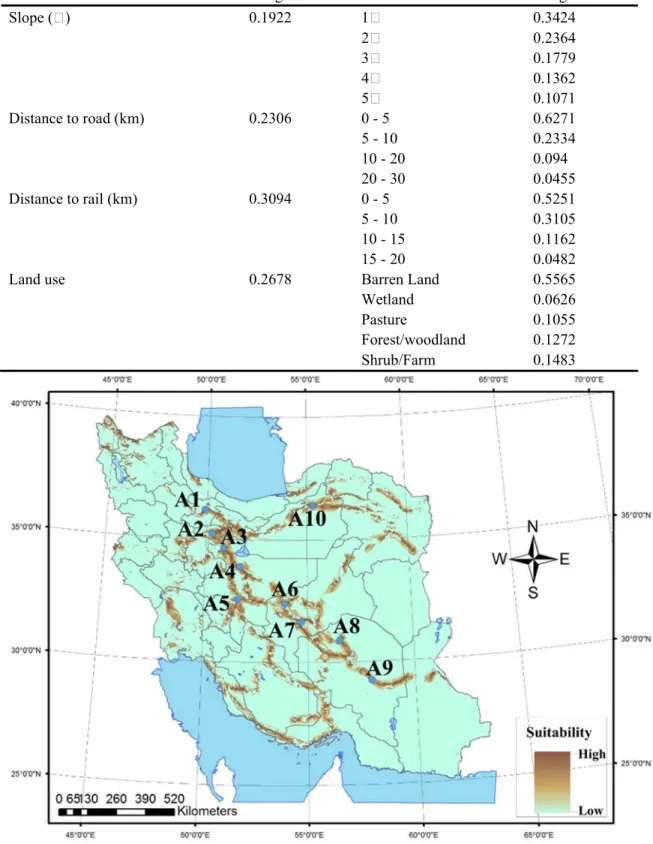
After preparing the aforementioned geographic layers, first, the level of suitability should be determined by moving away from the ideal values in each layer. For example, the closer to the road routes, the more suitable the location would be, while being away from the roads reduces suitability. Thus, the places are reclassified based on their distance from the routes. Once the layers are reclassified, the importance (weight) of the layers relative to each other was determined based on the experts’ opinions (table 3). Using the command “overly” in ArcGIS software, the obtained geographic layers were combined with each other according to the determined weights using AHP method and the final map was obtained (figure 2). According to figure 2, the potential points written to be introduced into the mathematical model included A1 to A10, which were extracted with respect to the experts’ opinions and the final GIS map. It should be noted that since this case study was aimed to construct the distant dry ports, the points close to the coast were not taken into account.
Table 3. Weights determined for indices and sub-indices to be used in selecting suitable locations
Criteria Weight Sub-criteria Weight
Slope (⁰) 0.1922 1⁰ 0.3424
2⁰ 0.2364
3⁰ 0.1779
4⁰ 0.1362
5⁰ 0.1071
Distance to road (km) 0.2306 0 - 5 0.6271
5 - 10 0.2334
10 - 20 0.094
20 - 30 0.0455
Distance to rail (km) 0.3094 0 - 5 0.5251
5 - 10 0.3105
10 - 15 0.1162
15 - 20 0.0482
Land use 0.2678 Barren Land 0.5565
Wetland 0.0626
Pasture 0.1055
Forest/woodland 0.1272
Shrub/Farm 0.1483
Fig. 2. Final map of selecting suitable locations for establishing dry ports
After determining the location of the potential points using GIS, these points were considered as parameters in the written mathematical models. The model was solved with a
deterministic and robust approach considering the data published by Iranian Ministry of Roads and Urban Development for demand values (table 4) and using CPLEX 12.5 solver in GAMS optimization software by a PC with CPU Intel Core i5-6267U.
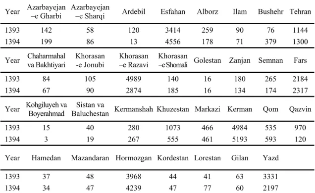
Table 4. Parameter of demand points
Year Azarbayejan –e Gharbi Azarbayejan –e Sharqi Ardebil Esfahan Alborz Ilam Bushehr Tehran
1393 142 58 120 3414 259 90 76 1144
1394 199 86 13 4556 178 71 379 1300
Year Chaharmahal va Bakhtiyari Khorasan -e Jonubi Khorasan –e Razavi Khorasan –e Shomali Golestan Zanjan Semnan Fars
1393 84 105 4989 140 16 180 265 2184
1394 67 90 2874 185 16 134 174 2317
Year Kohgiluyeh va Boyerahmad Baluchestan Sistan va Kermanshah Khuzestan Markazi Kerman Qom Qazvin
1393 15 40 280 1073 466 4984 535 970
1394 3 19 267 555 461 5193 593 120
Year Hamedan Mazandaran Hormozgan Kordestan Lorestan Gilan Yazd
1393 37 48 3968 44 41 63 3331
1394 34 47 4239 47 77 60 2197
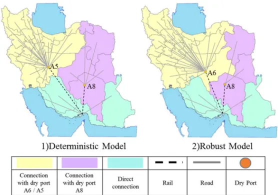
According to figure 3 representing the final results obtained from solving the mathematical model, points A8 and A6 in the robust mode and points A8 and A5 in the deterministic mode were determined as the final points for establishing the dry ports, the connection of each of the provinces with the seaports was provided directly or using the dry ports, and the demand was met.
Fig. 3. Optimal network of export and import demands in Iran by establishing dry ports in deterministic and robust models
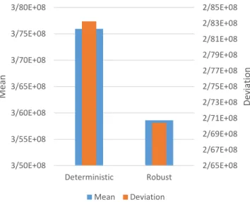
In this article, to compare the two deterministic and robust models, the simulation method was used so that using the uniform distribution, 15 random numbers (α) were generated and, accordingly, a value between the maximum and minimum demand data in the past four years was determined. Then, each of the robust and deterministic models was executed 15 times per nominal value for each of the produced demand parameters based on the solutions obtained from executing the model and the simulation results were reclassified into three parts (α >0.6, 0.3<α<0.6, α<0.3) according to the value of the random number. According to figure 4 through 6, when most of the demand parameters took their maximum values (figure 6), performance of the robust model was better demonstrated and the saving rate of this model became more obvious; however, in the case of lower demand, the difference between the robust and deterministic models was shown to be insignificant. However, according to figure 7, after the simulation, as expected, the mean and standard deviation of the robust model were less than those of the deterministic model and the model demonstrated more stability against the changes caused by the simulation. In other words, regarding the presence of the demand non-deterministic parameter, the robust model led to better results, which were closer to the optimal solution; but by applying the demand changes, the deterministic model showed more deviation from the optimal solution. Thus, the proposed robust model was more efficient in the uncertainty conditions.
Fig. 4. Performance of deterministic and robust models after simulation (0.3> α)
Fig. 5. Performance of deterministic and robust models after simulation (0.6>α>0.3)
Fig. 6. Performance of deterministic and robust models after simulation (1>α>0.6) 0/00E+00
2/00E+07 4/00E+07 6/00E+07 8/00E+07 1/00E+08 1/20E+08 1/40E+08 1/60E+08 1/80E+08 2/00E+08
0 1 2 3 4 5 6
Ob
je
cti
ve
Funct
ion
Deterministic Robust
1/50E+08 2/00E+08 2/50E+08 3/00E+08 3/50E+08 4/00E+08 4/50E+08 5/00E+08
0 1 2 3 4 5 6
Objective
Func
tion
Deterministic Robust
5/30E+08 5/80E+08 6/30E+08 6/80E+08 7/30E+08 7/80E+08 8/30E+08
0 1 2 3 4 5 6
Obj
ecti
ve
Fu
ncti
on
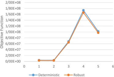
Fig. 7. Investigating mean and standard deviation of deterministic and robust models in actualization conditions The presented mathematical model was exogenous; thus, the number of the dry ports to be established was given to the model and the model could not make decisions on the number of them due to the constraints such as budget. Although the present case study sought to establish two dry ports, according to figure 8 for sensitivity analysis, each of the deterministic and robust models was implemented for different numbers of the established dry ports (P). By increasing the number of the dry ports from 1 to 5, the values of the objective functions were decreased, but the rate of this downward trend was reduced so that the objective function was further reduced by changing the number of the dry ports from 1 to 2. Investigating the changes in the objective function according to the changes in the number of the dry ports to be established might change the decision-maker’s opinion on determining the number of dry ports. It should be noted that changing P led to fewer changes in the robust model than the deterministic one.
Fig. 8. Changes in the objective functions of robust and deterministic models for changes in the number of established dry ports
2/65E+08 2/67E+08 2/69E+08 2/71E+08 2/73E+08 2/75E+08 2/77E+08 2/79E+08 2/81E+08 2/83E+08 2/85E+08
3/50E+08 3/55E+08 3/60E+08 3/65E+08 3/70E+08 3/75E+08 3/80E+08
Deterministic Robust
Dev
iatio
n
Me
an
Mean Deviation
0/7 0/75 0/8 0/85 0/9 0/95 1 1/05
0 1 2 3 4 5 6
Cha
nges
in
the
object
iv
e
funct
ion
(%)
Number of dry ports to be established (P)
4-1- Managerial insights
Regarding the considerable importance of port cities as good investment opportunities with a high risk-taking power, the investigation of relevant decisions and effective factors on them more than ever should be considered. Meanwhile, using the dry port as a multi-modal terminal to reduce the costs, maintain the competitiveness of the seaports, and suppose the seaports as a hub port in the main international shipping line is inevitable.
Solving the environmental problems is one of the most important social requests in 21 century (Lättilä et al., 2013) so that the reduction of carbon dioxide emissions in the country investigated in this paper is the main part of the government action plans. As noted in the present paper, with respect to the benefits like reducing the traffic jam in the port cities and intercity roads and also achieving multi-modal transportation, using dry ports in the countries’ logistics network can help to governments in the way of solving these problems.
Regarding the dry port is an emerging concept especially in the developing countries, the governments can encourage exporters and importers to use dry port by offering cheaper or more quality services and laying down government policies.
As mentioned before in sensitivity analysis section, the more the number of dry port established, the lower the cost of the transportation network. On the other hand, due to the too high cost of dry port establishment, depending on conditions and trade-off between the costs (establishment and transportation network costs) and benefits of the more establishment of dry port, relevant authorities should make suitable decisions. The geographic range of in question country and its transportation costs are included these conditions that the present paper proposed establishing two dry ports with respect to the conditions of the case study.
5- Conclusions
Dry port is a combined terminal in the hinterland, which is connected to one or more seaports using various methods of transportation. In addition to the basic services provided in this unit, the services such as commodities storage, maintenance of empty containers, customs affairs, and clearance are provided.
For establishing dry ports, factors such as land slope, land use, and proximity to roads and railways are of great importance, which are not taken into account in the models. Thus, in the present research, using GIS and investigating the geographic layers, Iran was reclassified into appropriate points for establishing dry ports and, then, these points were inserted in the mathematical model as the parameters of the potential points. Subsequently, in the mathematical model, the location of the dry ports was carried out with regard to the costs as well as the diffusion of pollution caused by various transportation methods. Due to the existence of the uncertainty in the demand parameter, the robust approach was used to deal with the uncertainty. Finally, after linearization, the model was solved using the idealistic programming approach for the case study of Iran; then, each of the deterministic and robust models presented some appropriate points for establishing the dry ports.
Despite all the advantages of the dry ports, establishing these terminals is very costly; thus, the private sector prefers to use such terminals in a stepwise manner in order to overcome high establishment costs. While such a consideration is of great importance, it is not seen in any of the published articles, so there is no solution for it. If the establishment of these ports in the model is broken into various levels with different profits and costs, it will become more applicable and get much closer to the reality; i.e. the model is authorized to choose which phase of the dry port should be established and opened at which time in order to achieve its maximum profit.
Another notable point that can be considered is to take into account other possible elements for freight transportation, including marine and air lines, because due to the novelty of the studies in this field, researchers have often used the railway transportation in combination with
the road transportation for connecting dry ports to seaports. However, regarding the above-mentioned concepts, the use of other transportation methods might lead to reduced costs and increased efficiency.
Moreover, the fuzzy approach has been highly regarded in the related articles that don’t use mathematical programming model; On the other hand, the articles proposing a mathematical model have not tended toward fuzzy approach, while it is very realistic and highly considered by industrial managers.
The proposed model can be further improved by incorporating dynamic service portfolio selection, considering other transportation modes like air and marine, and assuming fuzzy approach for various factors e.g. demand.
References
Alçada-Almeida, L., Coutinho-Rodrigues, J., & Current, J. (2009). A multiobjective modeling approach
to locating incinerators. Socio-Economic Planning Sciences, 43(2), 111-120.
Ambrosino, D., & Sciomachen, A. (2014). Location of mid-range dry ports in multimodal logistic
networks. Procedia-Social and Behavioral Sciences, 108, 118-128.
Aronsson, H., & Huge Brodin, M. (2006). The environmental impact of changing logistics structures.
The international journal of logistics management, 17(3), 394-415.
Ben-Tal, A., & Nemirovski, A. (2000). Robust solutions of linear programming problems contaminated
with uncertain data. Mathematical programming, 88(3), 411-424.
Beresford, A., Pettit, S., Xu, Q., & Williams, S. (2012). A study of dry port development in China.
Maritime Economics & Logistics, 14(1), 73-98.
Bertsimas, D., & Sim, M. (2004). The price of robustness. Operations research, 52(1), 35-53.
Chang, Z., Notteboom, T., & Lu, J. (2015). A two-phase model for dry port location with an application
to the port of Dalian in China. Transportation Planning and Technology, 38(4), 442-464.
Charnes, A., Cooper, W. W., & Ferguson, R. O. (1955). Optimal estimation of executive compensation
by linear programming. Management science, 1(2), 138-151.
Church, R. L. (2002). Geographical information systems and location science. Computers & Operations
Research, 29(6), 541-562.
Commission, E. (2000). IQ – intermodal quality final report for publication, Transport RTD
programme of the 4th framework programme – Integrated transport chain. Retrieved from
Crainic, T. G., Dell’Olmo, P., Ricciardi, N., & Sgalambro, A. (2015). Modeling dry-port-based freight
distribution planning. Transportation Research Part C: Emerging Technologies, 55, 518-534.
Cullinane, K., Bergqvist, R., & Wilmsmeier, G. (2012). The dry port concept–Theory and practice.
Maritime Economics & Logistics, 14(1), 1-13.
Dadvar, E., Ganji, S. S., & Tanzifi, M. (2011). Feasibility of establishment of “Dry Ports” in the
developing countries—the case of Iran. Journal of Transportation Security, 4(1), 19-33.
Do, N.-H., Nam, K.-C., & Le, Q.-L. N. (2011). A consideration for developing a dry port system in
Ehrgott, M., Gandibleux, X., & Przybylski, A. (2016). Exact Methods for Multi-Objective
Combinatorial Optimisation Multiple Criteria Decision Analysis (pp. 817-850): Springer.
El Ghaoui, L., Oustry, F., & Lebret, H. (1998). Robust solutions to uncertain semidefinite programs.
SIAM Journal on Optimization, 9(1), 33-52.
Feng, X., Zhang, Y., Li, Y., & Wang, W. (2013). A Location-Allocation Model for Seaport-Dry Port
System Optimization. Discrete Dynamics in Nature and Society, 2013.
Garivani, A., & Pishvaee, M. S. (2017). Honey global supply chain network design using fuzzy
optimization approach. Journal of Industrial and Systems Engineering, 10(3).
González-Sánchez, G., Olmo-Sánchez, M. I., & Maeso-González, E. (2015). Effects of the
Implementation of Antequera Dry Port in Export and Import Flows Enhancing Synergies in a
Collaborative Environment (pp. 147-154): Springer.
Gorsevski, P. V., Donevska, K. R., Mitrovski, C. D., & Frizado, J. P. (2012). Integrating multi-criteria evaluation techniques with geographic information systems for landfill site selection: a case study using
ordered weighted average. Waste management, 32(2), 287-296.
Haralambides, H., & Gujar, G. (2011). The Indian dry ports sector, pricing policies and opportunities
for public-private partnerships. Research in Transportation Economics, 33(1), 51-58.
Ignizio, J. P. (1983). Generalized goal programming an overview. Computers & Operations Research,
10(4), 277-289.
Jaberi, N., & Rafeh, R. (2014). On the Linearization of Zinc Models. Journal of Advances in Computer
Research, 5(4), 1-8.
Jaržemskis, A., & Vasiliauskas, A. V. (2007). Research on dry port concept as intermodal node.
Transport, 22(3), 207-213.
Kovacs, G., Spens, K., & Roso, V. (2008). Factors influencing implementation of a dry port.
International Journal of Physical Distribution & Logistics Management, 38(10), 782-798.
Lättilä, L., Henttu, V., & Hilmola, O.-P. (2013). Hinterland operations of sea ports do matter: dry port
usage effects on transportation costs and CO 2 emissions. Transportation Research Part E: Logistics
and Transportation Review, 55, 23-42.
Leveque, P., & Roso, V. (2002). Dry port concept for seaport inland access with intermodal solutions.
Master's Thesis, Department of logistics and transportation, Chalmers University of Technology.
Li, Z., Ding, R., & Floudas, C. A. (2011). A comparative theoretical and computational study on robust counterpart optimization: I. Robust linear optimization and robust mixed integer linear optimization.
Industrial & engineering chemistry research, 50(18), 10567-10603.
Malczewski, J. (1999). GIS and multicriteria decision analysis: John Wiley & Sons.
Malczewski, J. (2004). GIS-based land-use suitability analysis: a critical overview. Progress in
planning, 62(1), 3-65.
Mohseni, S., Pishvaee, M. S., & Sahebi, H. (2016). Robust design and planning of microalgae
Munford, C. (1980). Buenos Aires–Congestion and the dry port solution. Cargo Systems International: The Journal of ICHCA, 7(10), 26-27.
Ng, A. K., Padilha, F., & Pallis, A. A. (2013). Institutions, bureaucratic and logistical roles of dry ports:
the Brazilian experiences. Journal of Transport Geography, 27, 46-55.
Ng, A. Y., & Gujar, G. C. (2009). Government policies, efficiency and competitiveness: the case of dry
ports in India. Transport Policy, 16(5), 232-239.
Novy, D., & Taylor, A. M. (2014). Trade and uncertainty. Retrieved from
Parola, F., & Sciomachen, A. (2005). Intermodal container flows in a port system network:: Analysis
of possible growths via simulation models. International journal of production economics, 97(1),
75-88.
Qiu, X., & Lam, J. S. L. (2014). Optimal storage pricing and pickup scheduling for inbound containers
in a dry port system. Paper presented at the 2014 IEEE International Conference on Systems, Man, and
Cybernetics (SMC).
Qiu, X., Lam, J. S. L., & Huang, G. Q. (2015). A bilevel storage pricing model for outbound containers
in a dry port system. Transportation Research Part E: Logistics and Transportation Review, 73, 65-83.
Roso, V. (2007). Evaluation of the dry port concept from an environmental perspective: A note.
Transportation Research Part D: Transport and Environment, 12(7), 523-527.
Roso, V., & Lumsden, K. (2009). The dry port concept: moving seaport activities inland. UNESCAP,
Transport and Communications Bulletin for Asia and the Pacific, 5(78), 87-102.
Roso, V., & Lumsden, K. (2010). A review of dry ports. Maritime Economics & Logistics, 12(2),
196-213.
Roso, V., Woxenius, J., & Lumsden, K. (2009). The dry port concept: connecting container seaports
with the hinterland. Journal of Transport Geography, 17(5), 338-345.
Şener, Ş., Şener, E., Nas, B., & Karagüzel, R. (2010). Combining AHP with GIS for landfill site
selection: a case study in the Lake Beyşehir catchment area (Konya, Turkey). Waste management,
30(11), 2037-2046.
Soyster, A. L. (1973). Technical note—convex programming with set-inclusive constraints and
applications to inexact linear programming. Operations research, 21(5), 1154-1157.
Teixeira, J., Antunes, A., & Peeters, D. (2007). An optimization-based study on the redeployment of a
secondary school network. Environment and Planning B: planning and Design, 34(2), 296-315.
UNCTAD. (1991). Handbook on the Management and Operation of Dry Ports. Geneva.
Veenstra, A., Zuidwijk, R., & van Asperen, E. (2012). The extended gate concept for container
terminals: Expanding the notion of dry ports. Maritime Economics & Logistics, 14(1), 14-32.
Wang, C., Mu, D., Zhao, F., & Sutherland, J. W. (2015). A parallel simulated annealing method for the
vehicle routing problem with simultaneous pickup–delivery and time windows. Computers & Industrial
Engineering, 83, 111-122.
Wang, X., Yu, S., & Huang, G. (2004). Land allocation based on integrated GIS-optimization modeling
Wolf, A. (1995). Import and hedging uncertainty in international trade. Journal of Futures Markets,
15(2), 101-110.
Woxenius, J., Roso, V., & Lumsden, K. (2004). The dry port concept–connecting seaports with their
hinterland by rail. ICLSP, Dalian, 22-26.
Zachariadis, E. E., Tarantilis, C. D., & Kiranoudis, C. T. (2015). The load-dependent vehicle routing
problem and its pick-up and delivery extension. Transportation Research Part B: Methodological, 71,
158-181.
Zeng, Q., Liu, Y., Yang, Z., & Yu, B. (2011). Optimization of Dry Ports Location for Western Taiwan
Straits Economic Zone. Paper presented at the Reston, VA: ASCEProceedings of the Eleventh