Variance Reduction in Global Illumination with Monte Carlo
Methods
Raymond Kim advised by Sanjoy Baruah
University of North Carolina at Chapel Hill
Abstract Monte Carlo methods are a class of numerical algorithms that depend on repeated samples of random variables to obtain results; the numerical solution to the problem at hand can converge to the analytical solution by increasing the number of samples. However, as the problem becomes more
complex, this procedure of reaching an accepted solution becomes inefficient: the problem may require higher orders of samples to achieve a single order of accuracy. Thus, variance reduction techniques exist
to alter our method of performing the Monte Carlo method to achieve a faster convergence rate and a more accurate approximation given the same number of samples. In this paper we evaluate several
variance reduction techniques of the Monte Carlo method and its application in the global illumination problem in computer graphics.
Introduction to Monte Carlo Methods
Background
The term Monte Carlo was first mentioned in the article ”The Monte Carlo Method” by Metropolis and Ulam
in 1949, just after the end of World War II [1]. The article considers a medium in which nuclear particles
have the capability of producing other particles depending on their position and energy. This system is
formulated by a set of integro-differential equations (equations involving both integrals and deriatives of
the function) known as the Boltzmann equations; however, the classical methods used to deal with these
equations were “extremely laborious and incomplete” such that the closed form solutions were unobtainable.
Instead, a statistical approach is taken by sampling single chains of events upon which an analysis of the
possible outcomes’ properties and distributions at various times can then be conducted.
The notion of solving problems through statistical means have existed long before the 20th century.
A variant of Buffon’s needle experiment involving trials to estimate the value of π was published in the
18th century [2]. Even more so, the theoretical foundations of this method can be dated back to the 16th
century with the formalization of the law of large numbers [3]. Since the Monte Carlo method by nature
is repetitive, its popularity and practicality as a numerical technique only rose with the advent of modern
computers. Note that performing the Monte Carlo method involves randomness which brings us to the topic
of (pseudo)random number generators. Although it is out of this paper’s scope, it should not be disregarded
and should be considered an important area of study.
Motivation
The previous section briefly describes the original motivation of the Monte Carlo method and the problem
that was solved. As discussed, the sheer difficulty of the problem can be a factor in why the Monte Carlo
to the problem of interest). Take for example, the evaluation of a definite integral. At one dimension, there
are many different quadrature techniques to approximate the value of the integral, most of which perform
better than the Monte Carlo method (which would require sampling the function at random points along the
domain). These techniques can be extended to evaluate higher dimensional integrals; however, the number
of function evaluations grow exponentially as the dimension increases. In this case, the Monte Carlo method
can prove to be useful as its result does not depend in the dimensionality of the problem.
Another motivation of the Monte Carlo method is its applicability in different fields of study. It serves as a
strong optimization technique when uncertainty is at play. We’ve seen how it can be used in mathematics and
physical sciences, but this method can also be seen in engineering, finance, artificial intelligence, computer
graphics, etc. The Monte Carlo method is also conceptually simple. When we want to find the expected
value of a die, we can estimate this empirically by performing repeated simulations by rolling the die and
combining our results to get an answer (this experiment can be found in the curriculum of many elementary
schools).
In short, the Monte Carlo method is a simple and intuitive yet powerful method that can be used to
solve the most challenging of problems.
Definition
There is no common consensus on the definition of a Monte Carlo method. Some have come up with
clas-sifications and distinctions while others have come up with qualifications on what the Monte Carlo method
should entail. Putting these details and discussions aside, a nice general statement describes this method as
“a numerical method of solving mathematical problems by the simulation of random variables.” [4] This will
involve drawing samples from probability distributions. A general objective is to find the expectationEof a
transformationf on a random variableX. This is equivalent in evaluating the integral as notated below:
E[f(X)] =
Z
Ω
f(x)p(x)dx
whereX falls under some probability density functionp(x) in some sample spaceΩ. Since these two
expres-sions are equivalent, we can use them interchangebly as done a few times in this paper.
Examples
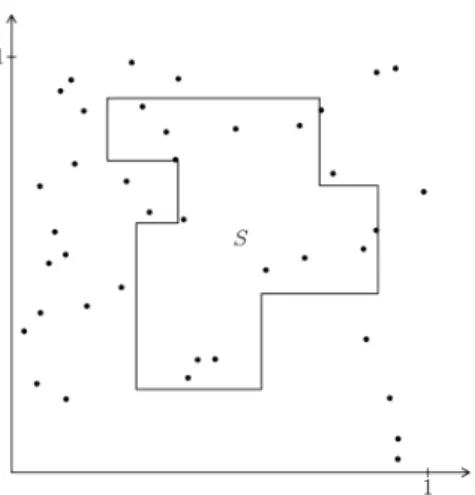
Figure 1.Estimating the area ofS
In the following examples we discuss how the Monte Carlo
method can be used to solve each problem. Note that we
for-mally do not know if the estimator for each example converges
to the right answer.Rather, we trust the correctness of each
estimator using intuition and common sense. The next section
hints at some of the underlying theory behind Monte Carlo
methods, but will focus on variance reduction techniques.
”Hit or Miss” method. This first example is simple but
does a nice job of showing how the Monte Carlo method can
be used to solve a basic problem. Consider an arbitrary plane
don’t need to know anything else about the figure, other than the fact that we can distinguish between points
in its interior and exterior. Our objective is to findE[S]. The spirit of the Monte Carlo method tells us that
if we take random points in our sample space enough times, then we can use
e
S= # points inS # total points
as an accurate estimator for S. For example, let us sample 40 points as shown in Figure 1, pulled from a
uniform distribution. There are 13 points inside S and thus we can estimateS by taking the ratio of the
two. This gives us an estimated area of 0.325 whereas the actual area (knowing the coordinates that were
used to plot this figure) is 0.3077. This gives us a relative error of about 5.6%. Taking 100 samples results
in a relative error of 0.75%.
We can see that this estimator does indeed work. Intuitively, we also understand that as we sample more
points, our estimator will become more accurate. Thix example can be extended into higher dimensions and
gives us an idea of how to use Monte Carlo methods to approximate the volume of high-dimensional bodies.
Simulation of a Mass Serving System. Consider a system of n lines that service incoming requests
arriving that moments
T1< T2<· · ·< Tk<· · ·
where thekth request comes at timeTk [4]. When the first request comes in, naturally, all the lines are free.
Hence, the first line will begin servicing the request for an arbitrary timeth. When thekth request comes in,
the first open line will start serving the request, but if all are busy then thekth request is considered rejected.
Our goal is to find the expected number of requests that are satsified and rejected. Analytically, solving this
may be tedious for a large number of requests. If we draw th from a distribution, then our problem may
become nontrivial and finding a solution becomes much harder. We can apply the Monte Carlo method here
to reach our objective; if we maintain a timer t we can essentially iterate through all Ti, updating t as we
go and keeping count of requests that are satisfied and rejected, so that in a single simulation, we get the
number of requests that are statisfied and rejected. Our Monte Carlo estimator can simply be the sample
mean of such simulations; by running it multiple times and taking the average, we can reach an esimate of
the expected values we are interested in.
Evaluating a Definite Integral On a more analytical end, let us try to find the integral of a simple
functionf where we define f to be
f(x, y) = exp(sin(8x2+ 3x) + sin(11y)).
We want to find
I= Z 1
0
Z 1
0
f(x, y)dx dy= Z 1
0
Z 1
0
exp(sin(8x2+ 3x) + sin(11y))dx dy.
In a more graphical sense, we want to find the volume created by this function over the unit square. Intuitively,
we can define our estimator to be
e
I= 1
N
N X
i=1
where Xi and Yi are random variables drawn from the uniform distribution U(0,1). In this sense, we can
estimate I by repeated sampling the function at different points throughout the domain. Here we see a
Figure 2.Heatmap of f (left) and 100 samples off (right)
heatmap off in the figure to the left and the result of 100 samples in the figure to the right. Although we
do not provide a complete numerical analysis, we see that we calculateIeby taking the average of all 100
sample values.
Variance Reduction Techniques in Monte Carlo Methods
Premise
There are two theorems that are fundamental to the Monte Carlo method, and the reason why we can expect
it to work. The first is stated as follows [5]:
Strong Law of Large Numbers. Let X1, X2, . . . be pairwise
indepen-dent iindepen-dentically distributed random variables withE[Xi]<∞. LetE[Xi] =µ andYn =X1+· · ·+Xn. Then,Yn/n→µalmost surely asn→ ∞.
Here we see that essentially as the number of samples we take approaches infinity, the sample mean approaches
the true expected values. In the previous examples, we used the sample mean as our estimator; by this theorem
we know that our this will converge to the correct answer and our estimator is indeed accurate. The second
theorem fundamental to studying Monte Carlo methods stated below:
Central Limit Theorem (Lindeberg-Levy). Suppose {X1, X2, . . .} is
a sequence of independently and identically distributed random variables
withE[Xi] =µand Var(Xi) =σ2<∞.Asn→ ∞,
√
n
1
n
n X
i=1
Xi !
−µ
!
→ N(0, σ2).
In otherwords, for{X1, X2, . . . , Xn} andYn =X1+· · ·+Xn, if nis
Simply put, the Central Limit Theorem states that the sum of a large number of identical and independently
distributed random variables will approximately fall under a normal distribution. The two theorems are very
similar in nature, but the difference between the Law of Large Numbers and the Central Limit Theorem is
that the latter tells us the shape of the distribution as well, which is helpful when evaluating variance.
Since the Monte Carlo method is based upon random variables, it is natural to expect variance in our
results. As mentioned earlier, the objective of the basic Monte Carlo method is to find some expectation
E[X] of a random variableX with variance σ2; we do so by collectingnsamples,X1, . . . , Xn, and using the sample mean as our estimator
Xn = 1
n
n X
i=1
Xi.
We find the variance of the basic estimator using the Central Limit theorem as follows:
Var(Xn) = Var 1 n n X i=1 Xi ! = 1 n2 n X i=1
Xi= 1
n2nσ 2= σ2
n.
The rate of convergence that signifies how fast the error is reduced is measured through the standard
deviation, which means that the rate of convergence for the basic Monte Carlo estimator becomesO(1/√n).
As we can see, the most obvious way to reduce our variance is by increasingn. Understandably, this does not
result in a very fast convergence rate and can be inefficient when comparing the cost necessary to generate
our samples versus the reduction in variance. Thus, we want to find methods in which we can alter our
sampling method or come up with a new estimator so that the error converges faster than our basic case.
Antithetic Variates
Using antithetic variates as a means of variance reduction involves introducing a negative correlation within
our samples [6]. Similar to our previous examples, suppose we are trying to find E[X]. Take Xi to be a random variable among the samples we take in the Monte Carlo scheme, where Xn was used as our basic
estimator. Assume the total number of samples nto be even so that we let n = 2m for some m ≥1. We
define Yi as the average betweenX2i−1 and X2i for i= 1,2, . . . , m and use Ym to be our new estimator.
Note the following:
Xn= 1 2m
2m X
i=1
Xi= 1
m
m X
j=1
Yj=Ym.
Here we see that the two estimators are equivalent, and thusYm can be used to findE[X]. We know that
Var(Yi) = Var
X2i−1+X2i 2
=1
4(Var(X2i−1+X2i)) = 1 4(σ
2+σ2+ 2 Cov(X
2i−1, X2i))
=1 2(σ
2+ Cov(X
2i−1, X2i)
| {z }
correlation
).
The coefficient is expected as there are half as many Yi as there are Xi. Thus, if we are able to pair up
samples ofXi such that the two are negatively correlated, then our covariance value becomes negative and
our overall variance is reduced.
There are several drawback to this method. First, we need to come up with a method of generating good
of this method is based upon an entirely different issue. There are problems in which generating antithetic
pairs are simple and straightforward; however, in most cases it will take some effort in doing so. Another
drawback is that if the sample pairs are poorly picked, then the correlation value becomes positive and our
varianceincreases. This is natural since picking simlar values will lower the amount of ’information’ we get compared to the ’information’ from two independently drawn samples. Thus, we need to be careful in how
we choose our antithetic samples when using this as a variance reduction technique.
Importance Sampling
Importance sampling alters the way we shoose our samples. In all of our previous scenarios, we assume that
the samples are drawn from a uniform distribution. The key idea behind importance sampling is choosing
samples from a probability density function that reflects the ”importance” of a sample’s contribution [4].
Assume that we want to evaluate the integral of some functionf(x) in some spaceA. If we let our probability
density fuction be denoted byp(x), then we wantpto be as close tof as possible. To see how this works,
we redefine the problem to be the following:
I= Z
x∈A
f(x)dx= Z
x∈A
f(x)p(x)
p(x)dx= Z
x∈A
f(x)
p(x)p(X)dx=E f(X)
p(X)
.
To find this value, we simply define an estimator to be
f
fnp(X) = 1
n
n X
i=1
f(Xi)
p(Xi)
where Xi is drawn from p(x). It has been shown that the variance is reduced most when p(x)∝ |f(x)|[4].
This can be easily checked by allowing p(x) =cf(x) for a constant c; taking the variance of the estimator
results in evaluating the variance of a constant 1/cwhich is 0. When solving forc, we solve the integral
Z
x∈A
p(x)dx= Z
x∈A
cf(x)dx= 1
which becomes the problem we are trying to solve. Finding the best probability density function is extremely
difficult, as the problems we use Monte Carlo methods to solve involve complex or black-box functions. It’s
often impractical to find the ”perfect”p, so we usually settle for finding apthat resemblesf. Similar to the
previous variance reduction technique, ifpis chosen poorly, this can lead to an increase in variance (consider
the case wherep(x) = 1/f(x)).
Stratified Sampling
As the name may imply, stratified sampling involves partitioning the sample space into different strata [7].
We find the expectation of each local strata, then combine the results to estimate our overall expectation.
Again, let us try to estimate µ = E[X]. Instead of taking n samples, we take l samples from m different
strata so that n = lm and let Xij be the value of theith sample from the jth strata [9]. We define the
estimator in thejth strata and our overall estimator to be
e
Xj= 1
l
l X
i=1
Allow the expectation and variance of the random variables per strata be denoted asµj andσ2j respectively.
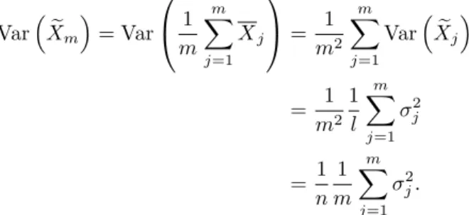
Using these definitions, we evalute the variance of our estimator to be
VarXem = Var 1 m m X j=1 Xj = 1 m2 m X j=1
VarXej = 1 m2 1 l m X j=1
σ2j
= 1 n 1 m m X j=1
σj2.
We similarly evaluate the variance for the basic estimatorX in terms of thej strata:
Var X=E
h
X2i−µ2= 1
m m X j=1 E h
X2|X from strataji−µ2
= 1
m
m X
j=1
(µ2j+σ2j)−µ2
= 1
m
m X
j=1
((µj−µ)2+σ2j)
≥ 1
m
m X
j=1
σj2.
It is clear to see that the variance of the stratified estimator is less than the variance of the basic estimator.
Intuitively, through stratifeid sampling we are reducing the variance that can exist between each strata. This
specific type of variance can be a result of an issue known as sample clumping where randomly generated
samples are clustered in one area; by partitioning the sample space we guaranteed some measure of spread
about our space. This is visualized in the figure below.
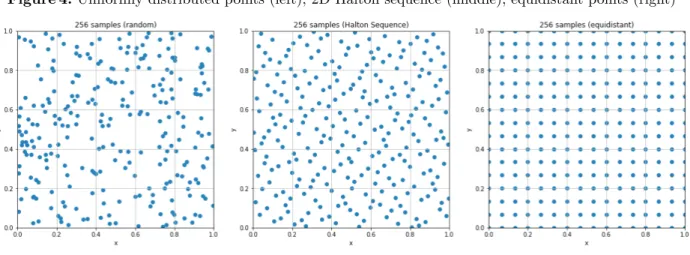
The Quasi Monte Carlo Method
This variance reduction technique is a bit different from the rest, as we do not depend on taking random
samples from a distribution. Instead, we use low discrepancy sequences to generate our samples. A low
discrepancy sequence is a deterministic sequence that share properties of random variables so that each
element is, as the term quasi is defined, seemingly random. These sequences are generated using prime
numbers and different number bases; a few famous ones are the Halton sequence, Hammersley set, and the
Sobol sequence. The rate of convergence for error using the Quasi Monte Carlo [8] is calculated to be
O
(logn)s
n
for some dimensions.
When compared to the convergence for the basic Monte Carlo method, we can see an improvmement when
nis high andsis relatively low.
Figure 4.Uniformly distributed points (left), 2D Halton sequence (middle), equidistant points (right)
The Global Illumination Problem
In global illumination, our objective is to accurately capture the light within an environment to generate
realistic images. From a light source, light rays will intersect with the scene, bounce around, and eventually
reach the camera where the image can then be formed. Global illumination involves the two types of
illu-mination: direct and indirect illumination. Direct illumination occurs when a position in the environment is
directly exposed to the light source whereas indirect illumination occurs when a position in the environment
is exposed to light that has been reflected from other surfaces. This problem has been formalized into what
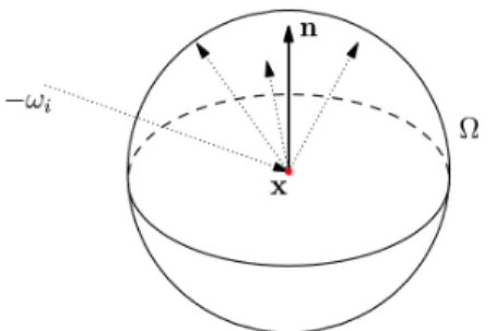
is known as the rendering equation [10,11]:
Lo(x, ωo, λ, t)
| {z }
outgoing radiance
=Le(x, ωo, λ, t)
| {z }
emitted radiance
+ Z
Ω
fr(x, ωi, ωo, λ, t)
| {z }
BRDF
Li(x, ωi, λ, t)
| {z }
incoming radiance
(ωi·n) | {z }
scalar
dωi
where x is the location in space, ωo is the direction of the outgoing light, λ is the wavelength of light, t
is time, ωi is the negative direction of the incoming light, and n is the surface normal at x. The BRDF
hits the surface. The domain of of the intgral is the hemisphere oriented about nand we take the integral
with respect to all incoming light rays.
Our interest lies in evaluating the integral in the right hand side of the rendering equation. Doing so
analytically is impractical as the scene can be arbitrarily complex, so we use the Monte Carlo method to
obtain an approximation. This requires a method of sampling differentωiaboutΩ, taking multiple samples,
performing the appropriate function evaluations, and calculating the sample mean to use as our estimator.
We now discuss two common methods used to do so: ray tracing and path tracing. Ray tracing establishes the
foundations of how the rendering will work, then path tracing extends upon that idea to solve the rendering
equation.
Ray Tracing
The term ”ray tracing” has evolved into a very broad term, but we will referring to the basic method proposed
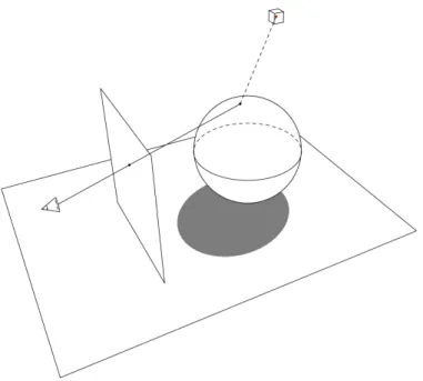
by Whitted in 1979 [12]. In ray tracing, we start from the camera (the cone in Figure 5) and intersect viewing
rays through the image plane and into the scene. This image plane is a figurative plane that the scene will
project onto (and will be our resulting image on a pixel by pixel basis). When the ray intersects the scene at
some positionx, we trace the ray fromxto the light source(s) (cube in Figure 5) in the scene - if the ray is
uninterrupted, then we include that light source when determining the amount of light gathered atx(which
determines the color for the pixel in the image). If the ray is interrupted (e.g. if the viewing ray intersects
the darkened area on the bottom plane of Figure 5), we ignore the light source when calculating the light
at that point which results in a shadow effect. A ray tracer can be extended to be recursive: in doing so,
Figure 5.Camera setup in a scene
we can achieve effects like reflection or perhaps even some basic caustics. However, one of the downsides to
ray tracing is that only direct lighting can be computed; this limits the features of our rendering to the ones
mentioned previously. There exist shortcuts and workarounds that can be applied to our basic ray tracer in
order to get more intricate details; however, this requires indepth knowledge about the scene and an artistic
eye to imitate such realism. Another requirement for a ray tracer are intersection functions for each object
defined analytically, it is required to know where each ray intersects with the object given any orientation.
As the scene becomes more complicated, this intersection function becomes costly which is a reason why ray
tracing has been mostly used for offline rendering. Other rendering methods exist in cases where latency is
an important issue (e.g. video-games, VR displays). With the rise in GPU’s and parallel processing power,
real-time raytracing has become feasible, allowing for beautiful renderings of virtual worlds.
Path Tracing
The second method, path tracing, is similar to that of ray tracing but has more of a probabilistic aspect
[10]. Before we discuss the algorithm and its implementation, we first need to understand the behavior of
light in a scene and indirect lighting. On a bright sunny day, it is obvious to see that the shadow of a tree
is not pitch black. This ambient lighting comes from what we call indirect illumination: light from a source
reaches an object and scatters around the environment, providing light to other objects in the scene. In the
example of the tree, the light ray may hit a nearby stone and get reflected into the leaves and then reach
ground where the tree’s shadow is located. If we relate back to the rendering equations, this is why we take
the integral with respect to the incoming light rays about the hemisphere.
Figure 6.Scattering of light rays atx
With this behavior in mind, path tracing makes an attempt at simulating the bouncing behavior of light.
Forward path tracing starts from the light source and follows the paths of light into the scene, keeping
track of all the light rays that reach our camera. However, this is really inefficient which is why we consider
backwards path tracing. Similar to ray tracing, we from the camera and shoot viewing rays into the scene.
However, instead of shooting a single ray through each pixel, we send a large number of rays through the
image plane. This number is often referred to as samples per pixel (SPP) and is a common metric for path
tracers; the number of samples can reach into the tens of thousands (resulting in a better image but slower
runtime). Next, for each ray, we find the intersection of the ray and the scene at some location x. In ray
tracing we checked whether or not x is exposed to any light. However, in path tracing, we bounce the ray
randomly within the hemisphere about the surface normal (the domain of our integral) as depicted in Figure
6. Of course, how we determine our reflected ray depends on the material and the BRDF atx: if the surface
is completely reflective then we can calculate the appropriate mirrored ray. If the surface is not perfectly
reflective, then we can choose a random ray that is biased towards the general direction of the mirrored
ray. Finally if the surface was perfectly diffuse, then we send the ray in a uniform random direction about
the hemisphere. Finally, if the viewing ray intersects with the light source, we can factor this back into the
original radiance value ofx. If the viewing ray never intersects with the light source given some upper bound
of bounces, then it is left alone.
Ideally, we want to take multiple samples per bounce and take the average to get a better estimate of the
otherwise the runtime will exponentially increase (for each of the thousands of original rays, we creatennew
rays). If we assume that we have the computing power to sample the hemisphere at multiple locations even
at high SPP, then it is essential to use a quality Monte Calo estimator to evaluate our integral.
Variance in Global Illumination
We see how Monte Carlo methods are used in path tracing and in solving the rendering equation, but
the problem we focus on is the variance associated with approximating the integral. In computer graphics,
variance comes in the form of visual artifacts: noise and aliasing. Noise resembles the random pixal pattern
from analog TV sets and is produced through the use of random numbers. In path tracing, if we use a low
SPP value then there can be a high likelyhood that a majority of those samples will miss the light source and
return a darker radiance than the true value. This is why images with low SPP values tend to look darker
in general.
When it comes to variance reduction techniques in global illumination, stratified sampling is one of the
more popular methods to reduce noise. Importance sampling and antithetic variates requires an indepth
knowledge about the scene we are rendering. Use of antithetic variates would require us to find negatively
corrleated sample pairs which is difficult for a single scene. Even more so, in the film industry, the scene we
are trying to render is constantly changing which makes importance sampling and antithetic variates even
more difficult to use. On the other hand, stratified sampling would be used to partition the hemisphere into
subregions from which samples will be taken. There is no need for knowledge about the scene we are trying to
render which is extremely convenient. Quasi-Monte Carlo methods have become an area of interest, as it can
have a faster convergence rate due to the low dimensionality of the problem [12]. A benefit of Quasi-Monte
Carlo methods in global illumination is that it can visually produce less noice, but can give way to aliasing
due to the periodic nature of low discrepancy sequences. Aliasing can be identified by unusual or out-of-place
patterns in our final render.
Sampling Technique Proposal
For the remainder of this report, I propose a proof of concept for a method using low-discrepancy sequences
to generate samples in our hemisphere. Generating these samples is not a trivial task, as it is incorrect to
use uniform random variables as parameters for our sphereical coordinates and expect a uniform distribution
about the surface of the hemisphere. This brings us to my main objective: to sample the hemisphere using
low discrepancy sequences while preventing any potential aliasing artifacts that may incur by introducing a
variability factor in the sampling process. I make the assumption that we are sampling a perfectly diffuse
surface (and thus our samples are generated uniformly about the surface of the hemisphere). We assuming
the hemisphere has radius 1 and is centered at the origin with the surface normal vector oriented upwards.
We first generate a 3D and 2D low-discrepancy sequence cube and square oriented about the origin and
with length values of 2 (that is, an inscribed sphere will have radius 1). Call these set of pointsAandB. For
nsamples, generating these values will have a runtime ofO(n3) andO(n2) but is only used at the beginning
and is a constant factor. For each sample inAi, if |Ai| ≥1, we discard the sample and continue. By doing
so, we start from a point cloud in a cube and transform it into a sphere. We perform a similar process toBi,
dicarding those whose length is greater than 1. Once we are left with valid values forAiandBi, we normalize
Ai so that the points are projected onto the surface of the sphere. If theAi lies on the lower hemisphere, we
the upper hemisphere. Next, we calculate a unit vectoruthat lies in the plane orthogonal toAi. We use an
arbitraryu for the time being. We letv be the cross product of uand Ai which gives us a vector that is
orthogonal touandAi. We want to adjust the lengths ofuandvdepending on the density of the samples
- if samples are genereated pretty closely then ouruandvshould be low to effectivly ”cover” the distance
between each sample points. Usinguandvas a basis of sorts, our new sample is calculated by evaluating
Ai+Bi,xu+Bi,yv
where Bi,x and Bi,y is the x and y values of our sample Bi. In doing so, we a method of smapling our
hemisphere using low discrepancy sequences but add in a variability factor. The runtime of this method
will be similar to the speed up from using Quasi-Monte Carlo methods and should reduce the possibility of
aliasing artifacts.
Discussion
Potential problems that may occur is the amount of normalizing we are doing in the process. Square roots are
expensive operations on a low level, and performing this billions of times can add up and become a significant
overhead. Another issue is being able to realisticially test and analyze this method; could take possibly days
to generate a single render, depending on the number of samples we take. Finally, the periodicity of low
discrepancy sequences can lead to unexpected effects. The transformations we perform on each sample can
unknowingly lead to patterns which will inaccurately sample the hemisphere.
Future Work
For future work, the most immediate step would be to implement this process and conduct numerical tests to
make sure of its viability. The transformation of low discrepancy seuqences can potentially be an interesting
area of study, since they are ultimately deterministic despite being quasirandom. It would be nice to conduct
a rigorous study of error bounds and discrepancy, providing a formal argument for the correctness of the
References
1. Metropolis, Nicholas, and Stanislaw Ulam. ”The monte carlo method.” Journal of the American statistical
asso-ciation 44.247 (1949): 335-341.
2. Robert, Christian P. Monte carlo methods. John Wiley & Sons, Ltd, 2004.
3. Mlodinow, Leonard. The drunkard’s walk: How randomness rules our lives. Vintage, 2009. 4. Sobol, Ilya M. A primer for the Monte Carlo method. CRC press, 1994.
5. Klenke, Achim. Probability theory: a comprehensive course. Springer Science & Business Media, 2013.
6. Hammersley, J. M., and K. W. Morton. ”A new Monte Carlo technique: antithetic variates.” Mathematical
pro-ceedings of the Cambridge philosophical society. Vol. 52. No. 03. Cambridge University Press, 1956. 7. Kahn, Herman. ”Use of different Monte Carlo sampling techniques.” (1955).
8. Søren Asmussen and Peter W. Glynn, Stochastic Simulation: Algorithms and Analysis, Springer, 2007, 476 pages
9. Giles, Mike. Numerical Methods II. Oxford University Mathematical Institute
10. Kajiya, James T. ”The rendering equation.” ACM Siggraph Computer Graphics. Vol. 20. No. 4. ACM, 1986.
11. Immel, David S., Michael F. Cohen, and Donald P. Greenberg. ”A radiosity method for non-diffuse environ-ments.” ACM SIGGRAPH Computer Graphics. Vol. 20. No. 4. ACM, 1986.
12. Whitted, T. (2005, July). An improved illumination model for shaded display. In ACM Siggraph 2005 Courses (p. 4). ACM.