1213.pdf

ABSTRACT

JEFETIEY L. KING. Application of an ANOVA Model To Evaluate Occupational Exposure to Formaldehyde. (Under the Direction of Stephen M. Rappaport, Ph.D.)

Occupational exposure to formaldehyde was evaluated at a large chemical

facility. Of particular interest was the validity of so-called Homogeneous

Exposure Groups (HEGs) in which it is assumed that all individuals are exposed, on average, to the same level of contaminant. As a preliminary step a field study was conducted comparing the use of diffusion monitors to sorbent tubes for personal air sampling. Results from 26 matched pairs showed the two methods to be comparable [mean difference (badge - tube) = 0.03 ppm; mean (badge) = 0.17 ppm]. Six HEGs were formed based on job tasks and location. Using a

randomized design, multiple full-shift samples were collected (with monitors) from

representative workers in each HEG (127 measurements from 44 workers).

Application of an analysis of variance (ANOVA) model indicated that the total variation in exposure across the entire sample population was partitioned as follows: 79% within-worker, 8% between-worker (within HEG), and 13%

m

TABLE OF CONTENTS

INTRODUCnON...1

Defining an HEG...2

Purpose...3

METHODS and MATERIALS...5

Facility - Process Review...5

Job Title - Task Review...8

HEG Formation...10

Random Selection of Workers and Sample Days...14

Field Study Comparing Sampling Methods for Airborne Formaldehyde...16

Statistical Evaluation of Sampling Data...19

RESULTS...26

Tests ofLognormality...28

ANOVA Results...29

DISCUSSION...33

CONCLUSIONS...37

CITED REFERENCES...38

GENERAL REFERENCES...39

APPENDIX A...40

Floor Plans APPENDIXB...48

Randomization Procedure APPENDIX C...51

Sample Day By Date APPENDDCD...53

Field Study Data and Analysis APPENDIXE...56

HEG Sampling Data

ACKNOWLEDGEMENTS

I would like to thank my research advisor Dr. Stephen Rappaport for his

guidance and support, and for the wisdom he shared with me during my studies at the University of North Carolina. I am also indebted to Dr. Hans Kromhout for his statistical expertise, and to Drs. Michael Flynn and Lori Todd for their

time and critical review of this report.

I also appreciate the opportunity and advise I received from Stephen Kemp, Michael Buczynski, and all the personnel at the facility where the work for this project was conducted. Others I wish to thank for contributing to the effort include: Brian Cawley, Esther Johnson, Susan Rappaport, and Elaine

Symanski.

Lastly, I am eternally grateful to my wife Susie, for her love, devotion, and patience, to my son Matthew, for his smile, and to my parents and siblings, for their unconditional love and support over the last 28 years.

This project was conducted as part of a graduate training program and

was supported in part by a National Institute of Occupational Safety and Health

INTRODUCTION

One of the primary duties of an occupational hygienist is monitoring the work environment to determine levels of exposure to airborne contaminants.

Sampling campaigns are undertaken for a variety of reasons: to ensure

compliance with governmental occupational exposure limits (OELs), to establish

baseline levels of exposure, to evaluate the effectiveness of engineering controls,

and to provide exposure information for future epidemiological investigations.

Regardless of the reason for monitoring, it is important for the hygienist to collect

samples which accurately reflect the level of exposure and which are sufficiently

representative to allow meaningful decisions to be made regarding the exposures.

Much progress has been made in the last fifty years to improve the accuracy and

precision of environmental sampling methods. However, the issue of

representative sampling in the field of occupational health has much room for

improvement. While the idea of representative sampling is nothing new nor

conceptually difficult, the how-to and application of a method of representative

sampling still presents difficulties for the occupational hygienist.

The problem is two-fold: usually not every worker can be monitored at all

times, and there exists a great deal of variability in the level of exposure across a

population of workers in a given work environment. Furthermore, occupational

hygienists have a limited amount of time and resources to devote to workplace

monitoring. Thus it is important to structure the monitoring program such that a maximum amount of information regarding exposures can be obtained from a minimum number of samples, while maintaining an acceptable degree of

sometimes termed homogeneous exposure groups (HEGs), where it is assumed

that all workers within a group are exposed, on average, to the same level of

contaminant.

Defining an HEG

The American Industrial Hygiene Association's (AIHA) Exposure

Assessment Strategies Committee (1991) defines an HEG as follows:

"A group of employees who experience agent exposures similar enough that monitoring agent exposures of any worker in the group provides data

useful for predicting exposures of the remaining workers. Such groups are used in stratified sampling of workplace exposures, thereby improving the

power of statistical decision tools. The categorization of workers into such

groups often involves categorization by process, job description, and agents, although finer separation can be attained by further dividing on

the basis of task analysis."

While this definition provides a useful qualitative description of an HEG, it gives the reader no guidance in terms of a quantitative description of such a group. In

fact, even though the word "statistical" appears in the definition, to date this

group, nor any other consensus group in the field of occupational health, has

specifically dealt with the defining attributes of an HEG, from a statistical

viewpoint.

Rappaport (1991) addresses the issue of defining discrete exposure groups

from a statistical viewpoint by defining two other terms. First, the author defines

a 'monomorphic' group as "a collection of individuals whose mean exposures can

be adequately described by a single log-normal distribution (between-persons)."

A 'uniformly exposed' group of workers is then defined as "a monomorphic group

this definition of a uniformly exposed group is arbitrary and possibly too restrictive, it does provide a quantitative framework with which to assess the homogeneity of a given EGEG. A metric based on this definition is denoted by the

author as R0.95, b ^^ is presented in an upcoming section.

There are essentially two approaches one can use to establish HEGs. One

involves classification of workers a priori, based on observational techniques.

The other method groups workers subsequent to random sampling of exposures,

and is hence considered a ;7<95fenon (Rappaport, 1991).

An a priori classification of workers into discrete groups called "exposure zones" was described by Com and Esmen (1979). The concept involves

prospective assignment based on task, agent, and work process similarities. A randomly selected sub-group of workers within each exposure zone is

subsequently sampled and assumed to represent the level of exposure for the entire group.

Purpose

This study was initiated to evaluate occupational exposure to

formaldehyde at a chemical manufacturing facility using HEGs based on an

observational approach. Of particular interest is the uniformity of exposures to

workers within such an established HEG. To address this issue, several HEGs were formed a priori using information on occupational title, job tasks, and work location. Multiple full-shift, breathing zone samples were subsequently collected using a randomized design from a representative sub-group of workers within

each HEG. The homogeneity of the data is evaluated statistically by means of an

analysis allows a judgment to be made regarding the success of the observational approach in this case, and provides valuable information on the distribution of

exposures at this facility, to help guide future monitoring programs.

The work for this report was conducted during a ten week industrial

hygiene internship served at this facility. Given the limited time and resources

available, and the research nature of the project, it was not intended to be a

comprehensive assessment of all exposures at this facility. The focus of the study

was limited to potential formaldehyde exposure for a segment of the workforce, albeit that segment which was deemed to have the greatest potential.

First, results are presented from a field study comparing two methods of

I)ersonal sampling for airborne formaldehyde. The preliminary study was initiated

to demonstrate the efficacy of passive monitors relative to the pump-sorbent tube method, which traditionally had been the standard formaldehyde sampling

METHODS and MATERIALS

Facility - Process Review

The workplace monitored for this project is a medium-sized chemical

facility located in western New York State. The plant produces phenolic resin

(approximately 30 million Ibs./year) and phenolic molding compound

(approximately 50 million Ibs./year). The production of both materials involves

batch-type operations, with the ability to produce hundreds of different

formulations depending on the specific application. These resins are used, for

example, in the aerospace industry as thermal barriers, in the abrasives industry as

adhesives, and in the coatings industry as ingredients in paints and varnishes.

Molding compounds are utilized extensively in the automotive industry as brake

parts, pulleys, motor frames, and ashtrays.

The plant consists of about 40 buildings spanning 66 acres of land, though

only a few are actively involved in production. Phenolic resin is produced in two

separate buildings, while molding compound is produced in one building. The

facility employs 120 salaried and 240 hourly personnel.

Phenolic resins, in general, are the polymerization product of a

condensation reaction involving phenol and an aldehyde. The vast majority of

phenolic resins consist of the phenol-formaldehyde variety, which is the type

made at this facility. In particular, this plant produces two types of

phenol-formaldehyde resin: a one-stage resole, and a two-stage novolac.

A resole is produced by reacting phenol and excess formaldehyde (50%

charged with all reactants needed for the final polymer; specifically, enough formaldehyde is added to make the resin thermosetting, or infusible once heated to a certain temperature. Production of a novolac, on the other hand, involves a two-stage process where an acid catalyst and a portion of the necessary

formaldehyde (80%) are reacted with phenol. The first stage forms partially

reacted, low molecular weight linear polymers. At this point the resin is

considered thermoplastic, or fusible since application of heat will not chemically

alter the material. The remainder of the formaldehyde necessary for final cure is

added at a later time during the second stage, typically in the form of

hexamethylenetetramine, which decomposes in the presence of heat and moisture to formaldehyde and ammonia. The latter acts as a catalyst.

Once a kettle is charged with the reactants it is generally heated to a boil

and refluxed for an amount of time determined by the given formulation. Upon

reaching a desired end-point (e.g. viscosity or percent free formaldehyde

remaining), the kettle is rapidly cooled and dehydrated to remove water and

unreacted phenol, which prevents the resin from advancing beyond the desired stage. The cycle time for resin production at this facility ranges from several hours to several days, depending on the specific resin. Upon completion, the molten resin is transferred from the kettle and may or may not undergo further processing, again depending on the specific resin and customer specifications. If it is sold as a liquid resin, it will either be packed-out in 55 gallon drums, or

transferred directly to a tank wagon for transport. It may also be transferred to a tank farm for storage as a liquid.

Alternatively, the resin can be converted to a solid form via additional

solidify. The solid mass is pulverized using a crusher and hammer mill. Once pulverized, it may be packed-out into boxes or bags, or used to make molding compound. Flake resin is formed using either a drum dryer or a belt flaker,

depending on the type of resin (novolac or resole). Once formed, it too is either

packed out or used for molding compound production.

The other primary manufacturing process at this facility is the production

of phenolic molding compound. In this process, pulverized resin is mixed with

various fillers, lubricants, and plasticizers in large ribbon blenders. The resulting

mixture is fed onto a set of counter-rotating heated rolls, where the material is

transformed into a thermosetting compound. From there the material goes

through a grinder, a sifter, and another blender prior to pack-out in drums, boxes, or bags. Figure 1 depicts the process, from resin production to molding

compound production.

Finally, there are a multitude of other support activities performed by

personnel at this facility. A quality control lab provides analytical services for

raw materials and resins in various stages of production. Maintenance operations include a welding shop, an electrical shop, and a metal fabrication shop.

FORMALDEHYDE SUPPUY WIEIGH

TANK

PHENOL (^'^ fO«M*4.D(M*Qt HOLD TANK I I "O'-0'-« '

r^^l^

AC 10 PUMP

RELIEF DISK

z:r2_

"^ ' i COMOCNUR \COOLIMG nATEn OUT

r=PK

OLINCCOH ^—^---U—ͣ

---ͣ

^ COOtiNCCOOLINC PANS

Amvcvon It DLLS FINfS r\r\ RINDCR ͣ LCNOED t Resin

^-'"' I Molding

'^ Compound

OnUMFACKOUT INAL PRODUCT

Job Title - Task Review

DRUM Off fOA POSSlSLC RtTUAM TOMIvcn

D \ OS

An analysis of job tides and associated tasks was performed, focussing on

those which were judged to have the highest potential for formaldehyde

exposure. Information on job titles was obtained from a 'weekly locator,' which

listed all personnel (by job tide) and their weekly shift assignment, and from

interviews with personnel. Job task information was ascertained through

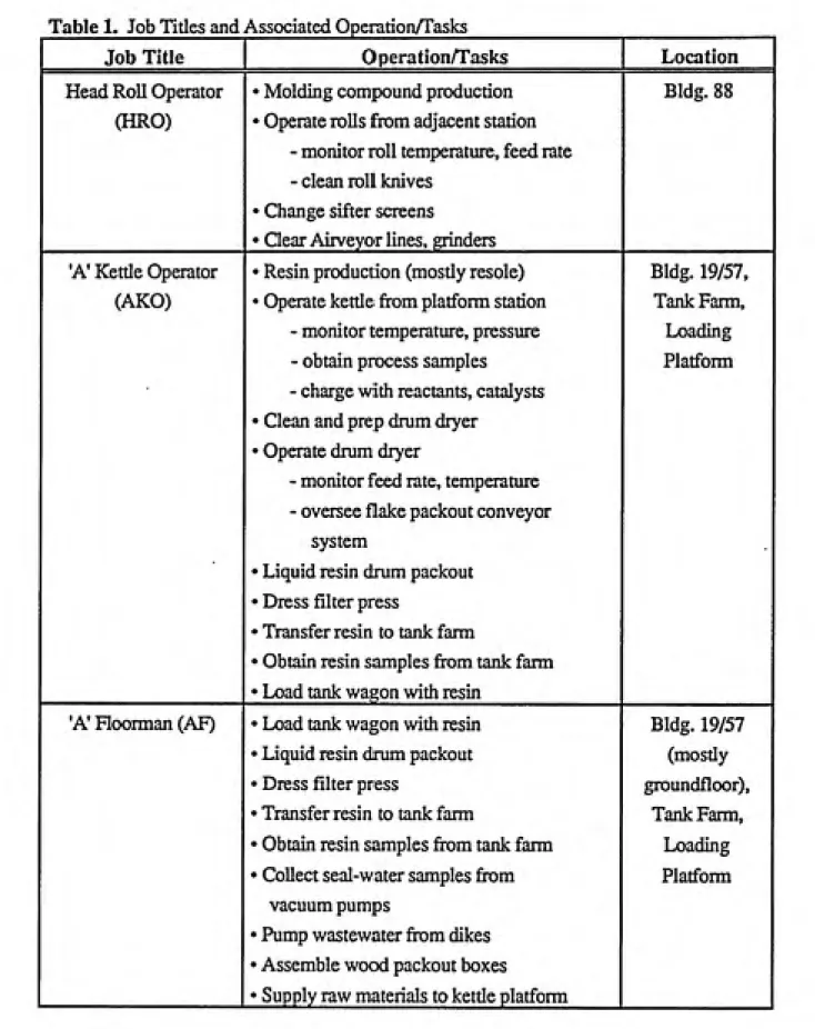
observation and interviews with personnel. Table 1 provides a summary of the

Table 1. Job Titles and Associated Operation/Tasks

Job Title Operation/Tasks Location

Head Roll Operator • Molding compound production Bldg. 88 (HRO) • Operate rolls from adjacent station

- monitor roll temperature, feed rate

- clean roll knives

• Change sifter screens

• Qear Airveyor lines, grinders

'A' Ketde Operator • Resin production (mostly resole) Bldg. 19/57, (AKO) • Operate kettle from platfonu station Tank Farm,

- monitor temperature, pressure Loading

- obtain process samples Platform

- charge with reactants, catalysts

• Clean and prep drum dryer • Operate drum dryer

- monitor feed rate, temperature

- oversee flake packout conveyor

system

• Liquid resin drum packout • Dress filter press

• Transfer resin to tank farm

• Obtain resin samples from tank farm

• Load tank wagon with resin

'A' Hoorman (AF) • Load tank wagon with resin Bldg. 19/57

• Liquid resin drum packout (mostly

• Dress filter press groundfloor).

• Transfer resin to tank fann _{Tank Farm,}

• Obtain resin samples from tank fanii Loading • Collect seal-water samples from Platform

vacuum pumps

• Pump wastewater from dikes

• Assemble wood packout boxes

10

Job Title Operation/Tasks Location

'A' Kettle Operator • Resin production (mosdy novolac)

• Operate kettle from platfonu station

- monitor temperature, pressure - obtain process samples

- charge with reactants, catalysts • Clean and prep belt or dram flaker

• Operate belt or dram flaker • Flake resin dram/box/bag packout

• Liquid resin dram packout

• Liquid resin pan job • Dress filter press

• Load tank wagon with resin

Bldg. 3/12

Lift Truck/Conveyor

Operator (LTO)

• Operate lift track - material transport

• Clean and prep belt or dram flaker • Operate belt or dram flaker

• Rake resin dram/box/bag packout • Liquid resin dram packout

• Liquid resin pan job • Dress filter press

• Load tank wagons with resin

Bldg. 3/12 (mostiy groundfloor)

Control Lab Specialist

(SFl)

• Run routine analyses on raw materials

and resins

- cures, titrations, pH, freeze point,

viscosity, refractive index, etc.

Control Lab

HEG Formation

After obtaining information on job title, task, and location, workers were

11

following four defining attributes of exposure zones (HEGs), as described by

Com and Esmen (1979):

1. Work similarity - workers in each HEG must perform similar job

tasks.

2. Hazardous agent similarity - workers in each HEG must share

potential exposure to the same agent(s).

3. Environment similarity - workers must perform job duties in similar

environments, such that exposures are influenced by similar controls

and processes.

4. Identifiability - there should exist a means of identifying workers

within an HEG to facilitate any future tracking efforts.

Based on these criteria, six HEGs were established, as presented in Table 2.

Table 2; Summary of Formaldehyde HEGs

HEG No. Job Classification Location No. of Workers

1 _{Head Roll Operator Bldg. 88 6}

2 _{A Kettle Operator Bldg. 3/12} 12

3 _{A Ketde Operator Bldg. 19/57} 28

4 _{Lift Truck/Conveyor Operator Bldg. 3/12} 4

5 AFloorman _{Bldg. 19/57} 6

6 _{Control Lab Specialist} Control Lab 12

Total 68

Each HEG represents a group of workers perceived to have a unique

potential for exposure to formaldehyde, given the job functions performed in the

specific work environment. In this case, each HEG represents a different job title,

or, for HEG 2 and 3, a different work location. It was not possible to further

define HEGs within job classifications based on job tasks, because of task

performed the same tasks based on a daily rotation procedure. Workers were not

"pigeon-holed" into performing specific tasks every shift; all tasks were rotated.

Therefore, it was assumed that all workers in a given job classification (and work

environment) over time were uniformly exposed and hence represented by a

discrete HEG.

HEG 1 is comprised of Head Roll Operators for Building 88, which

produces molding compound (see Appendix A for floor plan). It was estimated

that workers in this job classification are the only ones in the compound building

to have any significant potential for formaldehyde exposure. Formaldehyde, as a

raw product, is not present in this building. The job of a Roll Operator is to

monitor a set of differential rolls from an adjacent work station. Exposure may

occur as free-formaldehyde (unreacted) is vaporized during the heating of

pulverized phenolic resin as it is applied to the hot rolls. The amount of

free-formaldehyde present in a resin varies based on the given resin formulation and

the particular batch. Estimates of the percent of free-formaldehyde in resins

produced at this facility were as high as 14%, though the majority fall in the 0.5 to

5.0% range. Formaldehyde exposure for this job classification was also

dependant on the efficacy of the local exhaust ventilation (LEV) system for this

operation, which, it was noted, varied day to day. There were several factors

which seemed to influence its ability to remove generated contaminants. One

was process equipment operation, which itself was dependent on many factors,

such as the relative proportion of resin to fillers, the temperature of the rolls, the

relative humidity, and the feed rate. If conditions were not optimal, the process

generated contaminants in excess of what the LEV system could handle, resulting

in releases to the work environment. The other factor which influenced the LEV

system was the presence of air-flow disturbances, primarily cross-drafts from large

13

HEGs 2 and 3 are made up of Kettle Operators. Their job is to produce

phenolic resins. This facility has two separate resin production buildings, each of

which tends to make a different type of resin. Building 3/12 makes mostiy two-step novolac resins, while Building 19/57 produces mostly one-two-step resoles (see Appendix A for floor plans). Given the different work locations and the fact that

each building makes a different type of resin, two separate HEGs were formed,

one for the Kettle Operators in each building. Because formaldehyde is one of two primary raw materials used in the production of phenolic resins, this job

involves a number of exposure opportunities, even though it is primarily a closed

system. For example, charging kettles with formaldehyde can result in releases to the work environment when the manway is opened to make a visual check or, as a result of minor leaks during transfer of the charge from the facility holding system to the weigh case or pressurized charge tank. Another task that may

involve significant release to the work environment is when a kettle is charged

with formaldehyde in solid form (paraformaldehyde). This requires addition

through an open manway and hence more direct contact. Collecting raw material or process samples presents another opportunity for exposure. Kettle Operators

in Building 19/57 also risk exposure while operating a drum dryer, which

converts liquid resin into flake form through a dehydration process. Other tasks

involving potential exposure opportunities include liquid resin packout and

cleaning filter presses. The exposures relating to most of these tasks are

influenced to some degree by LEV. However, the effectiveness of these systems

is dependent upon the same factors mentioned previously for the LEV system in the compound building.

Lift Truck/Conveyor Operators in Building 3/12 make up HEG 4. This job

requires operating a lift truck on the ground level of Building 3/12, as well as resin

exposure opportunities associated with this job, though not as numerous as for

Kettle Operators. Tasks with the highest potential for exposure include cleaning

the filter press and the belt flaker, liquid resin packout into drums, and liquid resin pan jobs. Also, these workers risk exposure simply by working on the ground

floor of this resin production building.

HEG 5 is comprised of A Floormen in Building 19/57. This job is roughly

analogous to the Lift Truck/Conveyor Operators in Building 3/12. It involves

packout duties on the ground floor of Building 19/57, supplying raw materials to

the kettle platform, and loading tank wagons with liquid resin. The main

difference is that these workers spend significantly more time outside loading

tankwagons and transferring resins to and from the tank farm.

Finally, HEG 6 includes Control Lab Specialists who work in the Control

Lab in Building 21 (see Appendix A for floor plan). These workers conduct

specification analyses on resin samples from Buildings 3/12 and 19/57. Samples

taken from kettles at various production stages may arrive at the lab at high

reaction temperatures, resulting in potential exposures for workers. Certain

analytical procedures, such as cure tests, also involve potential formaldehyde

exposure.

Random Selection of Workers and Sample Days

In order to make valid estimates of the distribution of formaldehyde exposures at this facility and to comply with assumptions inherent to the

statistical model used for data analysis, randomization was incorporated into the

sampling campaign. That is, workers to be sampled from each HEG were selected at random, as were the days on which to sample each worker. To ensure

^^"^^isff-'UH^m^

15

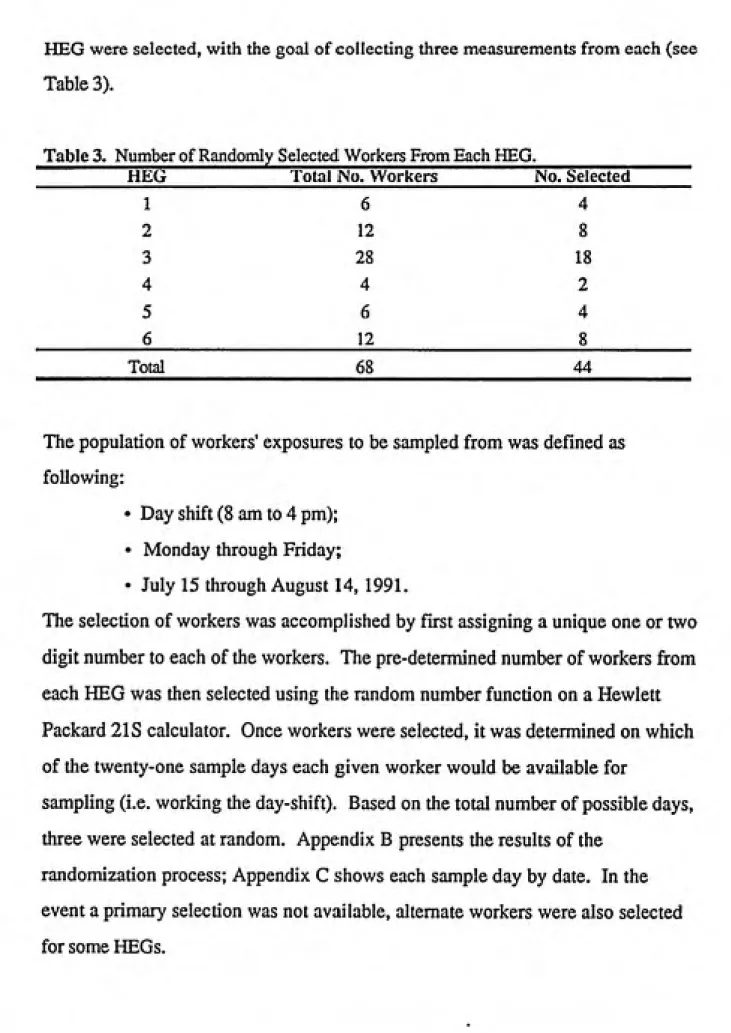
HEG were selected, with the goal of collecting three measurements from each (see Tables).

Table 3. Number of Randomly Selected Workers From Each HEG.________________ _________HEG_____________Total No. Workers__________No. Selected______

1 6 4 2 12 8 3 28 18

4 4 2 5 6 4

___________6_____________________12_____________________8___________

__________Total____________________68_____________________44__________

The population of workers' exposures to be sampled from was defined as following:

• Day shift (8 am to 4 pm);

• Monday through Friday;

• July 15 through August 14, 1991.

The selection of workers was accomplished by first assigning a unique one or two

digit number to each of the workers. The pre-determined number of workers from

each HEG was then selected using the random number function on a Hewlett Packard 21S calculator. Once workers were selected, it was determined on which of the twenty-one sample days each given worker would be available for

sampling (i.e. working tiie day-shift). Based on the total number of possible days,

three were selected at random. Appendix B presents the results of the

randomization process; Appendix C shows each sample day by date. In the

event a primary selection was not available, alternate workers were also selected

Field Study Comparing Sampling Methods for Airborne Formaldehyde

Prior to the random sampling of HEGs, a preUminary field study was

conducted to compare two personal sampling methods for airborne

formaldehyde. The study incorporated a matched-pair design and was initiated to

demonstrate the efficacy of passive diffusion monitors relative to the

pump-sorbent tube method.

The passive monitors utilized for this study were manufactured by Air

Quality Research (AQR), model PF - 20 (PEL). This device uses a dry proprietary

collector which converts formaldehyde to a stable intermediate, prior to

regeneration and analysis by the chromotropic acid method. It is designed to

monitor exposures for intervals ranging from one to eight hours. The monitors

were compared to sorbent tubes manufactured by SKC, model XAD - 2 (Treated).

These tubes also employ a dry collection media, but require the use of personal

sampling pumps to draw air through the device at a uniform rate. Sampling

pumps used were Gilian Personal Air Samplers with Constant Low Flow

Modules. Nominal sampling rate for 4-hour samples was 100 cc/min, and 50

cc/min for 8-hour samples. Pumps were calibrated before and after each sample

interval with a Mini-Buck Calibrator (Model M-5), and were checked periodically

in the field with a precision low-flow rotometer. Two field blanks of each type

were prepared each day and all samples were stored at 40-45°F. Soft bristle

brushes were used to remove any visible dust from outer membrane on diffusion

monitors prior to sealing. AQR monitors were analyzed by the manufacturer at

their facility in Research Triangle Park, North Carolina, while the SKC sorbent

tubes were analyzed by NATLSCO Environmental Sciences Laboratory located

17

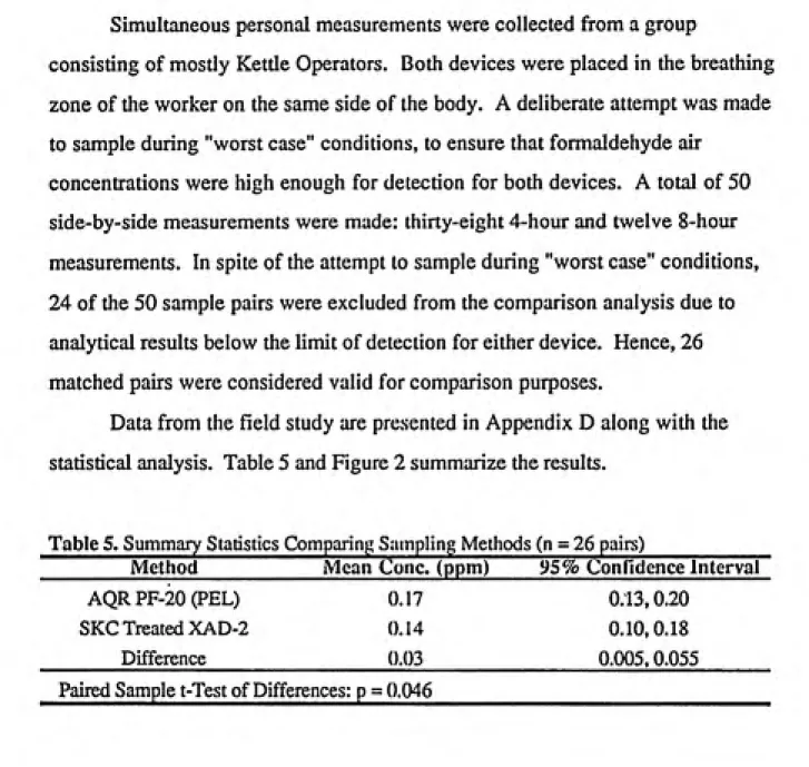
Simultaneous personal measurements were collected from a group

consisting of mosdy Kettle Operators. Both devices were placed in the breathing

zone of the worker on the same side of the body. A deliberate attempt was made

to sample during "worst case" conditions, to ensure that formaldehyde air

concentrations were high enough for detection for both devices. A total of 50

side-by-side measurements were made: thirty-eight 4-hour and twelve 8-hour

measurements. In spite of the attempt to sample during "worst case" conditions,

24 of the 50 sample pairs were excluded from the comparison analysis due to analytical results below the limit of detection for either device. Hence, 26 matched pairs were considered valid for comparison purposes.

Data from the field study are presented in Appendix D along with the

statistical analysis. Table 5 and Figure 2 summarize the results.

Table 5. Summary Statistics Comparing Sampling Methods (n = 26 pairs)___________

Method Mean Cone, (ppm) 95% Confidence Interval

0.13,0.20

AQR PF-20 (PEL) 0.17

)KC Treated XAD-2 0.14

Difference 0.03

0.10,0.18 0.005,0.055

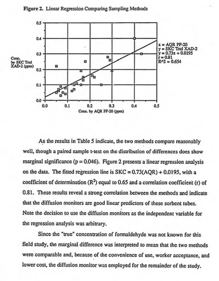
Figure 2. Linear Regression Comparing Sampling Methods

0.5

0.4

03

Cone.

by SKC Trtd 36U3-2(ppm)

0.2

0.1

0.0

---ij---B

a B

,...—»^

---B---B

_^y^

...IS...

1*^

< I

^"^

L-^

0.0 0.1 0.2 0.3 0.4

Cone, by AQR PF-20 (pirni)

X = AQR PF-20 y = SKC Trtd XAD-2 y = 0.73x + 0.0195 r = 0.81

R'^2 = 0.654

0.5

As the results in Table 5 indicate, the two methods compare reasonably

well, though a paired sample t-test on the distribution of differences does show

marginal significance (p = 0.046). Figure 2 presents a linear regression analysis

on the data. The fitted regression line is SKC = 0.73(AQR) + 0.0195, with a

coefficient of determination (R^) equal to 0.65 and a correlation coefficient (r) of

0.81. These results reveal a strong correlation between the methods and indicate

that the diffusion monitors are good linear predictors of these sorbent tubes.

Note the decision to use the diffusion monitors as the independent variable for

the regression analysis was arbitrary.

Since the "true" concentration of formaldehyde was not known for this

field study, the marginal difference was interpreted to mean that the two methods

were comparable and, because of the convenience of use, worker acceptance, and

19

Statistical Evaluation of Sampling Data

Sampling results were evaluated statistically with SAS software by means of an analysis of variance (ANOVA) based on the random effects model. This

model can be used to determine means and variance components for a given

variable based on repeated observations from a factor across numerous levels.

For example, estimating average exposures within and across groups of workers based on repeated measurements from each worker. For this study, two versions

of the model are used: a one-way classification, and a two-way nested

classification.

The one-way classification ANOVA was used to evaluate the exposure

variability within and between workers in each HEG. The equation for the model

is,

Yij = |I-H Ai-F Eij.

The term Yy represents the log-transformed exposure concentration received by

the ith worker during the jth sample interval (shift). The symbol \i is the mean

exposure for the population of workers, where Ai is the difference in mean

exposure of the ith worker from that of the population as a whole and ey is the

difference between each individuals' mean exposure (jij) and the exposure

received by that individual on any given day. The terms Aj and ey are both

2 2

assumed to be normally distributed with a mean of zero and variance ae and a^

2

respectively, and are considered independent. Thus oq represents the

between-2

worker component of variation, and Ow the within-worker component. It is also

assumed that)!, is normally distributed with a mean \i and variance Or, and that

the within-worker variance is uniform across all workers in the population.

Another assumption inherent to this model is that each observation is a random

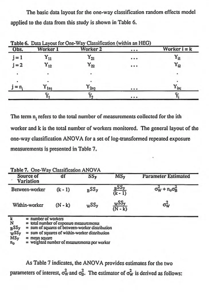
The basic data layout for the one-way classification random effects model

applied to the data from this study is shown in Table 6.

Table 6. Data Layout for One-Way Classification (within an HEG)_________________

Obs._____Worker 1________Worker 2___________;_;_;_________Worker i = k

j = 1 Yii Y21 ... Yji

j = 2 Y12 Y22 ... Yi2

J ="i_________Yin^______________Y2n2 ... _____________^^mj_______

_______________%________________%________________.^________________%

The term n. refers to the total number of measurements collected for the ith

1

worker and k is the total number of workers monitored. The general layout of the

one-way classification ANOVA for a set of log-transformed repeated exposure

measurements is presented in Table 7.

Table 7. One-Way Classification ANOVA Source of

Variation

df _{SSy MSy} Parameter Estimated

Between-worker

Within-worker

(k-1)

(N-k)

gSSy

wSSy

uSSy

(k-1) wSSy (N-k)

2 2

Oxv + noOg

k = number of workers

N = total number of exposure measuremcnus gSSy = sum of squares of between-worker distribution ^SSy = sum of squares of within-worker distribution MSy = mean square

Hq = weighted number of measurements per worker

As Table 7 indicates, the ANOVA provides estimates for the two

2 2 1

21

i J

wSy - wMSy - (N - k)

The quantity.

n

Yi =

lYi

i=l

Hi '

is the estimated mean of the i-th worker's log-transformed exposure measurements. The ANOVA estimator

computed from the following equation:

2

measurements. The ANOVA estimator for the other component of variance, as, is

2_ [(sMSy-vyS^)]

k 2

The term no= N - (LnJN) and represents the weighted number of measurements

i

per worker. Finally, because the total variance is simply the sum of the within and

between components, an estimate of the total variance is.

2 _ 2 2

T-Sy - ^Sy + gSy .

The two-way nested classification for the random effects model is used to

assess exposure variability not only within and between workers in a group, but

also between groups or, in this case, HEGs. The random effects model is

unchanged except for one additional term:

Yhij = |i + Bh + Ahi-H £hij.

For this model, Yhij is the log-transformed exposure concentration received by the

the mean across the entire group, but Bh represents random deviations of the

mean of the hth HEG about the grand mean and is normally distributed with mean

zero and variance anEG- As with the first model, the Ahi term corresponds to

between-worker deviations and £hij to within-worker deviations, and both are

normally distributed with a mean of zero and variance as and aw, respectively.

Finally, each term is assumed to be an independent variable and all measurements

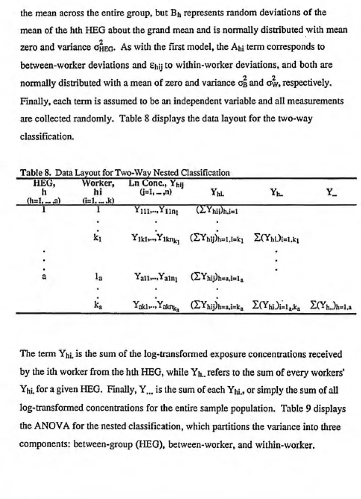
are collected randomly. Table 8 displays the data layout for the two-way

classification.

Table 8. Data Layout for Two-Way Nested Classification___________

HEG, Worker, Ln Cone, Yhy

h hi a=l,-,n) Yhi. Yh.

(h=l,... ,a)_____(i=l,... ,k)_____________________

i i Yiii,..,Yiini (ZYhii)h.i=l

ki Yiki,..,Yiknijj (SYhij)h=i,i=ki S(Yhi.)i=i,ki

Yaiiv.,Yaini (2)Yhij)h=a.i=la

Yakl.-.,Yaknk^ (ZYhij)h=a.i=ka X(Yhi.)i=i^jca S(Yh..)h=l,a

The term Yhi. is the sum of the log-transformed exposure concentrations received

by the ith worker from the hth HEG, while Yh.. refers to the sum of every workers'

Yhi. for a given HEG. Finally, Y... is the sum of each Yy., or simply the sum of all

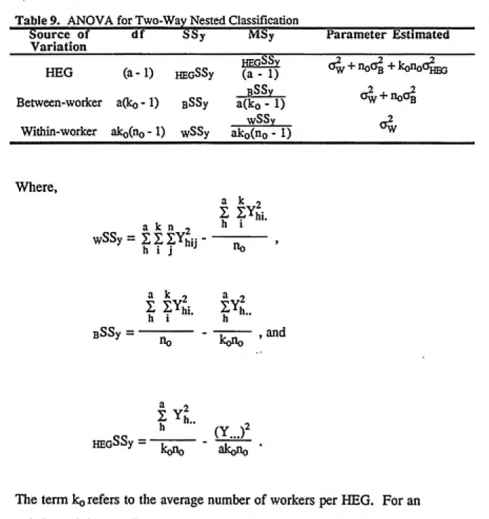
log-transformed concentrations for the entire sample population. Table 9 displays

the ANOVA for the nested classification, which partitions the variance into three

23

Table 9. ANOVA for Two-Way Nested Classification

Source of d^ _{^Sy MSy} Parameter Estimated

Variation

HEG _{(a-1) HEcSSy}

HEcSSy

(a- 1) <^w

+ Doag + koHoCJ^p,

Between-worker _{a(ko-l) sSSy}

sSSy

a(ko - 1) (% + noOg

Within-worker _{ako(no -1) wSSy}

wSSy

ako(no - 1)

elf

Where,

a k ^

I IYh':

a k n 2 ^ ^

wSSy = X Z I^hij

hi.

h i j '"J no

? ?^hi. SYJ..

iyJ..

________(Y...)

koUo akoUo

The term ko refers to the average number of workers per HEG. For an

unbalanced data set (i.e. unequal number of workers in each HEG, and unequal

measurements per worker), Uq and ko are estimated as follows:

(N-k

(S

i

n-)/ N)

, and

ilo-K - 1

ko =

a

Ik,

h

Where, K is the total number of workers sampled for the entire population, and A

is the total number of HEGs sampled. Thus, estimates of each component of

variance are:

wS? = wMSy = ajjnji),

2 _ fiMSy-wMSy

B^ - no

2

2 _ HEpMSy - wMSy - npeSy

HEcSy - k^n^

2222 222 2

Finally, the total variance ot = <^w + Ob + cjheg» hence jSy = ^Sy + gSy + ^^QSy.

To assess the degree of exposure homogeneity between workers within

HEGs and across the total group, a metric described by Rappaport (1991) was

used. The metric defines a 'uniformly exposed' group of monomorphic workers as

a group in which 95% of the individual mean exposures are within a factor of 2,

This implies that the ratio of the 97,5th percentile to the 2,5th percentile, denoted

by bRo.95. is not greater than 2, Where,

bRo.95 = exp [3.92 ag],

and Gg is the standard deviation of the between-worker distribution of the

log-transformed exposures. In this study, the true value of Gg was not known so the

estimate of bRo.95 (designated g R0.95) was used as the measure of uniformity.

This estimate,

25

2

where ySs is the between-person component of variance obtained from the

random effects ANOVA on the log-transformed measurements.

Clearly, the assumption that the exposure concentrations are lognormally

distributed is an important one. To verify the validity of this assumption, a formal

goodness-of-fit test was used, in addition to a less rigorous qualitative method.

The goodness-of-fit test employed for this study was the Shapiro-Wilk W test,

which is considered to be a statistically powerful and superior omnibus test of the

fit to the lognormal model (Waters, et al, 1991). AW statistic and corresponding

p-value was computed for each HEG and for the population as a whole,

A visual representation of the fit was also made by means of a

log-probability plot, where the cumulative probabilities are plotted against the

corresponding geometric mean exposure concentration for each worker across

the entire sample population. Each workers' cumulative probability was derived

from [i / (k + 1)], where i is the rank from low to high of each mean from the

between-worker distribution of k workers (Rappaport, 1992). Only balanced

data were used, that is, only cases with three measurements per worker. Due to

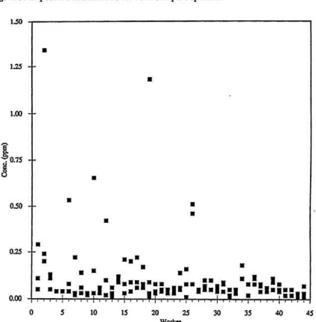
Results from the random sampling of the six HEGs are displayed in Figure

3 and are presented in tabular form in Appendix E. Each sample represents a

full-shift, 8-hour time-weighted average (TWA) concentration.

Figure 3. Exposure Measurements for Total Sample Population

1^

1.25

1.00

--I '0.75

0.50

0.25

--0.00

ͣ

I

10 15 20 25

Worker

27

A total of 130 measurements were made, two less than the desired number.

Table 10 accounts for the actual number obtained per HEG versus the number

desired.

Table 10. Measurements Collected Per HEG

HEG____________No. Desired________________No. Collected________

1 12 11 2 24 24 3 54 55

4 6 6

5 12 10

6 ______________24________________________24____________

Total_______________132_______________________130____________

For HEG 1, two of the four workers selected for monitoring were transferred to a

differentjobafter one measurement was made on each. Three samples were

subsequently collected for the alternate, as well as for the other two workers

originally selected. For HEG 3, a fourth measurement was made for one

previously selected worker, when a no-show from HEG 5 made available an extra

monitor on that day. Likewise, one other worker from HEG 5 did not show on

their scheduled day, resulting in a total of two measurements less than desired for

this group. It should also be noted that alternate workers, which were selected at

random, were used for HEGs 2 and 6. Finally, the samples from a worker

belonging to HEG 6 were excluded from the analysis because their job during the

sample interval was in a location different from that of the other workers in this

group. A temporary laboratory had been setup in one of the resin buildings.

Hence, the total number of measurements included in the analysis was 127, which

3 0.8787 0.3207

8 0.9328 0.5462

18 0.9226 0.1472

2 1.0 _1.0

2 1.0 _1.0

7 _{0.9776 0.9458}

Tests of Lognormality

Table 11 presents the results of the Shapiro-Wilk W test on the

goodness-of-fit of the data to the lognormal model.

Table 11. Results of Shapiro-Wilk W Test for Lognormality

HEG k W Statistic P Value

1

2

3

4 5

________6__________________________________________________________

Total Population__________40_____________0.9737____________0.5827

At an alpha level of 0.05, the null hypothesis of lognormality was not rejected for

any group. Clearly the test results for groups 1, 4, and 5 are without meaning,

given the small sample sizes. The degree of non-significance for the total group,

however, does indicate that the assumption of lognormality was reasonable, at

least for the total between-worker distribution of exposures. Further evidence

that the total group was monomorphic can be seen in Figure 4, which shows a

log-probability plot of the between-worker distribution for the total group. It

appears to be approximately linear. Finally, the results for groups 2, 3, and 6

indicate that the assumption of lognormality was reasonable, thus each can be

29

Figure 4. Log-Probability Plot for Total Between-Worker Distribution

i.

§

U

u

I

i

o

0.1

o:^-aO... 00

<P^

.00^.<^o

oo

QQI ' < < ' "'"^ I I r iiriiliiiii I . I I MiliiMiiirilriiili.iiluifliiiiln.rlri..li.iMi.iilrii I I...I,i... i liri.i,

0.01 0.1 1 5 10 20 30 4050 60 70 80 90 95 99 99.9 99.99

Cumulative % Less Than Indicated Cone.

ANQVA Results

Complete results from the analyses of variance performed on the exposure

measurements for these groups are presented in Tables 13-20. First, Table 12

provides a summary of the results. A total of seven one-way ANOVAs were

completed, one for each HEG and one for the total population, in addition to a

nested two-way analysis using HEGs as the primary factor. The one-way

classifications partition the variance into estimates of the within and between

m

classification reveals any reduction in between-worker variability as a result of

the grouping scheme, and is used to gauge the success of the process for this

population.

Table 12. Summary Statistics from One-Way Classification ANOVAs

HEG N k _{X (± sd)}

[ppm]

y

T^

(% of Total) (% of Total) B ^0.95

1 11 5 _{0.24 (± 0.38)} -2.08 1.129 _{0.712 (58.8) 0.498 (41.2) 15.9} 2 24 8 _{0.12 (± 0.17) -2.82} 1.226 _{1.215 (99.0) 0.012 (1.0) 1.5}

3 55 18 _{0.11 (±0.17)} -2.66 0.685 _{0.714 (100.0) - 0.030 (0.0)} 1.0 4 6 2 _{0.04 (± 0.02) -3.50 0.431}

0.369 (78.3) 0.102 (21.7) 3.5

5 10 4 _{0.09 (± 0.04) -2.56 0.381}

0.241 (58.4) 0.171 (41.6) 5.1

6 21 7 _{0.05 (± 0.03)} -3.28 0.439 0.308 (67.8) 0.146 (32.2) 4.5 Total 127 44 _{0.11 (± 0.18)} -2.77 0.841 _{0.691 (81.9) 0.152(18.1) 4.6}

N

k sd

k

w^

B*y

8^0.95

= number of exposure measurements per group

= number of woricers monitored = arithmetic mean

= sample standard deviation = mean of log-transformed data = total variance of log-transformed data = within-worker variance component = between-worker variance component

= estimated ratio of 97.5* and 2.5'*' percentile ftom the between-worker distribution

Table 13. One-Way Random Effects ANOVA for HEG 1

Variance Source df _{^S MS Variance}

Component

Percent of

Total

Between-Worker 4 7.0173 1.7543 0.4983 41.16

Within-Worker 6 4.2743 0.7124 0.7124 58.84

31

Table 14. One-WayRandom Effects ANOVA for HEG 2

Variance Source df SS MS Variance

Component

Percent of Total

Between-Worker 7 8.7534 1.2505 0.0119 0.97

Within-Worker 16 19.4364 1.2148 1.2148 99.03

Total 23 28.1898 1.2256 1.2267 100.00

Table 15. One-WayRandom Effects ANOVA for HEG 3

Variance Source df SS MS Variance

Component

Percent of

Total

Between-Worker 17 10.5860 0.6227 - 0.0300 0.00

Within-Worker 37 26.4253 0.7142 0.7142 100.00

Total 54 37.0113 0.6854 0.7142 100.00

Table 16. One-Way Random Effects ANOVA for HEG 4

Variance Source df SS MS Variance

Component

Percent of

Total

Between-Worker 1 0.6766 0.6766 0.1024 21.71

Within-Worker 4 _{1.4774 0.3694 0.3694}

78.29

Total _{5 2.1540 0.4308 0.4718}

100.00

Table 17. One-Way Random Effects ANOVA for HEG 5

Variance Source df SS MS Variance

Component

Percent of

Total

Between-Worker 3 1.9882 0.6627 0.1711 41.56

Within-Worker 6 1.4438 0.2406 0.2406 58.44

Table 18. One-Way Random Effects ANOVA for HEG 6

Variance Source df SS MS Variance

Component

Percent of Total

Between-Worker 6 4.4789 0.7465 0.1462 32.21

Within-Worker 14 4.3092 0.3078 0.3078 67.79

Total 20 8.7881 0.4394 0.4540 100.00

Table 19. One-Way Random Effects ANOVA for Total Population Variance Source df SS MS Variance

Component

Percent of

Total Between-Worker 43 48.6258 1.1308 0.1524 18.07 Within-Worker 83 57.3663 0.6912 0.6912 81.93

Total 126 105.9921 0.8412 0.8436 100.00

Table 20. Two-Way Nested Random Effects ANOVA for Total Population___________

Variance Source df SS MS Variance Percent of

________________________________________________Component______Total

HEG 5 15.1253 3.0251 0.1151 13.20

Between-Worker 38 33.5005 0.8816 0.0660 7.56

Within-Worker 83 57.3663 0.6912 0.6912 79.24

DISCUSSION

The sampling results clearly indicate that the vast majority of

formaldehyde exposures at this facility are well below the OSHA PEL of 1.0

ppm as an 8-hour TWA. In fact, out of 127 measurements, only two were above

the OEL (Figure 3, Appendix E). The mean exposure across the entire sample

population was 0.11 ppm with a standard deviation of 0.18 ppm.

Table 12 shows that the Head Roll Operators (HROs) in HEG 1 had the

highest mean exposure of all six groups (0.24 ppm), while HEG 4 had the lowest

(0.04 ppm). The analyses of variance reveal that for most groups and the

population as a whole, the total variation in exposures was predominantly

within-worker, that is, day-to-day. Estimates of the percent of total variation belonging

to the within-worker component ranged from 58.4% to 100.0 %. The low

degree of between-worker variation indicates relatively homogeneous exposure

conditions at this facility. However, using the definition of a uniformly exposed

group described earlier (i.e. g Rq 95 ^ 2), only two of the six groups would be

considered uniformly exposed: HEG 2 and 3. Given the extremely small

components of between-worker variation for each of these groups, accounting

for 1.0% and 0.0%, respectively, of the total variation, this result is not

A

surprising. Compared to the total population, with a g R095 of 4.6, the grouping

scheme reduced the g Rq 95 and the between-worker variation in four of the

HEGs. Yet, for groups 1, 4, and 5, with the total number of samples collected

34

These results also indicate that the between-worker variation across the

entire sample population was relatively low. In fact. Tables 12 and 19 show that

between-worker variance accounted for less than 20% of the total variance. This

implies that the subclassification of workers into discrete exposure groups, in an

effort to reduce variability between workers, would have limited effect for this

population since a "perfect" grouping would only account for about 20% of the

total variation across the population. Hence, a 20% reduction in exposure

variability is the most that could have been achieved through the use of HEGs.

As the nested ANOVA in Table 20 reveals, this effort was able to account for

roughly 13% of the total variation or two-thirds of the 20% which could be dealt

with in this manner.

In addition to providing information on the homogeneity of exposures, the

analyses of variance also offer insight on the nature of exposures at this facility.

Specifically, since the total variation in exposure across the entire population,

and for each HEG, was predominantly within-worker, exposures are governed

mostly by production processes or environmental conditions which are common

to the entire group. This implies that in general, individual jobs or work tasks

are not contributing to wide fluctuations in exposure to formaldehyde between

workers at this facility. Given the practice of rotating tasks within job classes,

this is, perhaps, to be expected.

However, the results indicating such a large degree of within-worker

variation (accounting for 99.0% and 100.0% of the total, respectively) for HEGs

2 and 3 was surprising. At first glance, the sampling results displayed in

Appendix E for these two groups do not appear to support this finding. Yet,

upon closer inspection, the fact remains that there were indeed very large

35

within-person differences were so large that for the statistical analysis,

differences between the means of individual workers were obscured.

So, the relevant question is why were day to day fluctuations in exposure

so great. One contributory factor may relate to the type of processes involved

with the production of resin at this facility, specifically the intermittent nature of

the operation. When resin undergoes production, kettles are charged, samples

are collected and analyzed, and product is processed; there is opportunity for

exposure. If kettles are not producing resin, there is minimal opportunity for

exposure. Clearly, exposures will fluctuate based on the production of resin.

Another factor which accounts for day to day variability is certain job tasks

performed fairly infrequently, but which can impact the level of exposure for

workers in an entire building. In particular, the task of charging a kettle with

paraformaldehye is not performed every day, but leads to higher exposures for

the majority of workers present in the building on those days when it is

performed. For example, on the July 30, Worker 1 from HEG 2 started the shift

that day by finishing the task of charging Kettle 323 widi paraformaldehyde (see

Appendix E). This operators' exposure on this day was 0.53 ppm, significantly

higher than the other measurements made for this worker on other days. In

addition, note that on this same day two other operators were monitored

(Workers 2 and 3), and their exposures were also higher than those received on

subsequent sample days. The end result is that this intermittent task contributed

greatly to the within-worker variation for each operator, yet did not confer a

large degree of between-worker variation.

Another factor which may have contributed to within-worker variance, by

and Floormen, from Buildings 3/12 and 19/57, respectively. However, the converse did not occur. That is. Lift Truck Operators or Floormen never performed tasks directly related to kettle operation. In any case, a potential consequence of task overlap is a reduction in between-worker variation, since performing similar tasks generally involves similar potential for exposure.

Finally, the fact that Head Roll Operators in HEG 1 received the highest exposures, on average, was unexpected, given that formaldehyde as a raw product is not present in Building 88. Formaldehyde is released, as described previously, during the heating of pulverized phenolic resin as it is applied to the nip of the heated rolls. Apparently, the process is capable of releasing more formaldehyde than the author thought possible, and the engineering controls are not adequately removing all of the contaminant generated. A brief investigation of the circumstances involved with the single exposure above the OEL received by a worker from this job class, revealed that the operator did experience

difficulties with the process on that day. The other possibility which might

account for the higher than expected results for this group is contamination of the monitor with resin dust, which is very prevalent for this process. It is

possible that dust trapped in the outer membrane of the monitor after it is sealed, continues to off-gas any free formaldehyde which was present in the dust.

However, there are two reasons why this possibility is thought to be unlikely.

For one, measures were taken to remove all visible dust from the outer

CONCLUSIONS

For this study, the use of diffusion monitors for full-shift personal

sampling of formaldehyde exposure provided results comparable to sorbent

tubes. Even though the monitors tended to read marginally higher compared to

the sorbent tubes, the benefits outweigh any loss in accuracy, if it actually exists.

The monitors require less labor, are more readily acceptable to workers, and are

more cost efficient. The end result is an increased number of samples, which

leads to a more accurate characterization of the distribution of exposures.

The observational approach used to assign workers to HEGs in this case

was only marginally effective. In terms of reducing between-worker variability

in exposures, the a priori groupings were successful for one-half of the groups

based on an analysis of variance of sampling results. However, the most

significant finding of this study was the fact that between-worker variability

accounted for only 20% of the total variation for the population.

Between-worker variation was obscured by the large degree of within-Between-worker variation,

or fluctuations day to day, which was likely a result of the batch nature of the

operation and task overlap between groups.

Given the relatively uniform exposure conditions between workers within

groups and across groups, much effort could have been avoided if the entire

population had been randomly sampled prior to the assignment of workers into

exposure groups which were perceived to be discrete. This illustrates the benefit

of an a posteriori approach to assessing exposures across a population of

American Industrial Hygiene Association, A Strategy for Occupational Exposure

Assessment AIHA, Akron, OH, 1991, p. 160.

Com, M., and Esmen, N.A., "Workplace Exposure Zones for Classification of Employee Exposures to Physical and Chemical Agents," American Industrial

Hygiene Association Journal. Vol. 40, Jan. 1979, pp. 47-57.

Kromhout, H., et ai, "Agreement Between Qualitative Exposure Estimates and

Quantitative Exposure Measurements," American Journal of Industrial Medicine.

Vol. 12,1987, pp. 551-562.

Rappaport, S.M., "Assessment of Long-Term Exposures to Toxic Substances in Air," Annals of Occupational Hygiene. Vol. 35, No. 1,1991, pp. 61-121.

Rappaport, S.M., "Interpreting Levels of Exposures to Chemical Agents," Patty's Industrial Hygiene and Toxicology. Vol. IIIA, 3rd Edition, In Publication.

GENERAL REFERENCES

Billmeyer, F.W., Textbook of Polymer Science. Wiley, New York, 1962.

Brown, B.W,, and Hollander, M., Statistics: A Biomedical Introduction. WUey,

New York, 1977.

Searle, S.R., Linear Models for Unbalanced Data. Wiley, New York, 1987.

Snedecor, G.W., and Cochran, W.G., Statistical Methods. Iowa State Univ. Press,

Ames, lA, 1989.

Walker, J.F., Formaldehyde. Krieger Publishing, Huntington, NY, 1964.

Woolson, R.F. Statistical Methods for the Analysis of Biomedical Data. Wiley,

41

Building 3/12 Floorplan - Ground Level

Office

Bay Door

Liq. Resin

Packout

Bay Door Bay Door

Drum Flaker

Flake Packout

mm]

/ Kettle \

^ Stairs to Platf(Min

Liq. Resin Packout

/ Kettle \

KZJ

Stairs to Platform

Kettle

301

nnnn

Ketfle

312

Belt Flaker

;:• ::

Flake Packout

Storage

Tank 344

O

Case

Bay Door

Building 3/12 Floorplan - Platform Level

Break Area

KetUe 323

to Ground

Floor

CH20 Charge

Tanks

OS.

Kettle 314

Vacuum

^-^ Pumps

B Stairsjo

E Ground Floor

^---"V, *

f Kettle \

Kettie 301

Balcony

Filter Press

Lockers

Storage

Legend:

O.S. = Operator Station

C.P. = Control Panel

S^^^^p^^

43

Building 19/57 Hoorplan - Ground Level

stairwell

Storage Tank

Liq. Resin Packout

KetUe

1914

Kettle 1912

Kettle

5708 Liq. Resin

Packout

Drum Dryer OJS.

Kettle 5709

Kettle

5713

Liq. Resin

Packout

{ Kettle \

I 5715 J

Flake Packout Conveyor System

J Tubes

m

Filter Pi (upst;

esses aprs)

Stairs

Bay Door Bay Door

Stairwell

Building 19/57 Floorplan - Platform Level

Legend:

O^. = Operator Station

C J*. = Control Panel

Stairwell

Kettle

1912 KetUe

1914

Kettle 5708

K5704 KS706

Kettle

5713 Kettle

5709

K5705 K5707

I KetUe 1

Office _OS.

m

45

Building 88 Floorplan - Ground Level

stairwell

Offke

Bay Doors

Ribbon Blenders

Compound Packout

Bay Door

Legend:

Building 88 Floorplan - Upper Level

stairwell

Rolls

Legend:

O.S. = Operator Station C.P. = Control Panel

Control Lab - Floorplan

47

Lab Hood \, Lab Hoods

Ovens

imni Qnnn Dnnn

Computer Room

Storage Room

1 Legend: 1

49

Appendix B Random Selection of Workers and Sample Days; Number of Samples Collected

HEG Worker Shift Selected _{Sample Days} Randomly Actual No.

ID No. (V) _{on Day Shift} Selected Sample Days

Samples

Collected

1 1 i ͣ 10-13 " 11,12,13 3

2 1

3 2 V 1-5,14-18 3,16,17 3

4 2 _V(Alt) 14-18 16,17,18 3

5 3

_i

6 3 V 6-9,19-21 8,19,20 1

2 ͣ 01 1 V ~ 10-13 ͣ 10,11,12 3

2 02 1

_i

2 03 1 _i 10-13 10,11,13 3

2 04 1 V 10-13 11,12,13 3

2 05 2

2 06 2 V 1-5,14-18 4,5,14 3

2 07 2 V 1-5,14-18 2,3,17 3

2 08 2

2 09 3 V 6-9,19-21 7,8,9 3

2 10 3 _V(Alt) 6-9,19-21 9,19,21 3

2 11 3

2 12 3

f

6-9,19-21 6,9,19 0

3 ͣ 01 V (Alt 1) 1-5,19-21 1,5,20

3 02

3 03

_i

3 04

_i

3 05 i 1-5,19-21 1,5,19 3

3 06 i 1-5,19-21 1,4,20 3

3 07

_i

3 08 K

, V

3 09 K V(Alt2) 14-18 15,16,18

3 10 K V 14-18 15,17,18 3

3 11 K

3 12 K V 14-18 14,15,17 3

3 13 K

3 14 K

_V,

3 15 L

_i

3 16 L V 6-9 6,7,8 3

3 17 L

_^

3 18 L V 6-9 7,8,9 3

3 19 L

3 20 L

3 21 L

3 22 M

3 23 M V 10-13 10,11,12 3

3 24 M V 10-13 10,11,13 3

3 25 M V 10-13 10,11,12 3

3 26 M V 10-13 10,11,12 3

3 27 M V 10-13 10,11,13 3

"HE(r Worker Shift Selected _{Sample Days Randomly} Actual No.

ID No. (V) on Day Shift Selected Sample

Days

Samples

Collected

4 1 1

4 2 2 V _1-5,14-18 3,14,16 3

4 3 3 V 6 - 9,19 - 21 19,20,21 3

4 4 3

5 1 J V " 1-5,19-21 3,4,19 2

5 2 K V 14-18 14,16,17 2

5 3 K

5 4 L V 6-9 6,7,9 3

5 5 M V 10-13 10,12,13 3

5 6 M

6 01 J "

6 02 J V _1-5,19-21 1,3,21 0

6 03 J V (Alt 1) 1-5,19-21 4,5,20 3

6 04 K V 14-18 14,15,17 3

6 05 K

6 06 K V 14-18 15,17,18 3

6 07 L i 6-9 6,7,8 3

6 08 L

_i

6 09 L

_i

6 10 M V 10-13 10,12,13 3

6 11 M _V(Alt2) 10-13 11,12,13

6 12 M V 10-13 11,12,13 3

Alt = Alternate in the event any selected worker was not available

* = Indicates day on which 4th sample was collected; worker was randomly selected to wear monitor after

Appendix C Sample Day by Date

Sample Day Date

1 _{July 15}

2 16

3 17

4 18

5 19

6 22

7 23

8 24

9 25

10 30

11 31

12 _{August 1}

13 2

14 5

.15 6

16 7

17 8

18 9

19 12

20 13

APPE^fDIXD

Appendix D Data from Sampling Methods Field Study and Statistical Analysis

AQR PF-20 (PEL) Cone. SKC Treated XAD-2 Cone. Difference [AQR - SKC]

(ppm) (ppm) (ppm)

0.09 0.04 0.05

0.14 0.11 0.03

0.18 0.25 -0.07

0.08 0.05 0.03

0.17 0.13 0.04

0.13 0.10 0.03

0.25 0.10 0.15

0.13 0.07 0.06

0.16 0.10 0.06

0.30 0.19 0.11

0.40 0.40 0.00

0.29 0.26 0.03

0.07 0.09 -0.02

0.07 0.03 O.M

0.43 0.30 0.13

0.22 0.15 0.07

0.16 0.19 -0.03

0.28 0.28 0.00

0.17 0.15 0.02

0.12 0.06 0.06

0.21 0.16 0.05

0.05 0.05 0.00

0.09 0.08 0.01

0.05 0.22 -0.17

0.06 0.07 -0.01

55

n = 26 Matched Pairs

Sample Mean:

AQR=:0.17ppm

SKC = 0.14 ppm

Difference (d) = 0.026 ppm

Sample Standard Deviation: AQR = 0.10 ppm SKC = 0.09 ppm Difference (s^) = 0.062

Paired Sample t-Test on Differences:

d-ix,

t = 2.105

Probability that 11| > 2.105 = 0.046

Result: At a 0.05 level of significance, borderline rejection of the null hypothesis

of no significant difference between the two methods.

HEG Worker ID Date 8-Hr TWA

No. (ppm)

Job Title PF-20 ID

No.

Location

(Bldg.)

Operation/Job Task

1 1 073191 0.13 HRO 1090359 88 Downstairs Rolls

1 1 080191 0.05 HRO 1090371 88 _{Downstairs Rolls/General Cleanup}

1 1 080291 0.11 HRO 1090383 88 _{Cleaned Pulverizers/General Cleanup/Downstairs Rolls}

1 3 071791 0.29 HRO 1090288 88 _{Upstairs Rolls/Cleaned Sifters}

1 3 080791 0.11 HRO 1090415 88 Upstairs Rolls

1 3 080891 0.05 HRO 1090425 88 Upstairs Rolls

1 4 080791 0.24 HRO 1090416 88 _{Main Floor Materials Handling/Downstairs Rolls}

1 4 080891 0.20 HRO 1090424 88 Downstairs Rolls

1 4 080991 1.34 HRO 1090431 88 Downstairs Rolls

1 5 072591 0.04 HRO 1090337 88 _{General CleanupAJpstairs Rolls}

1 6 072491 0.04 HRO 1090327 88 Packout Ehities

2 1 073091 0.53 AKO 1090347 3M2

2 1 073191 0.04 AKO 1090360 3\12

2 1 080191 0.08 AKO 1090380 3M2

2 2 073091 0.22 AKO 1090354 3M2

2 2 080191 0.03 AKO 1090372 3M2

2 2 080291 0.02 AKO 1090384 ?M2

2 3 073091 0.14 AKO 1090348 3\12

2 3 073191 0.06 AKO 1090367 3M2

2 3 080291 0.03 AKO 1090385 3\12

2 4 073191 0.02 AKO 1090361 3M2

2 4 080191 0.03 AKO 1090373 3M2

2 4 080291 0.03 AKO 1090386 3M2

2 6 071891 0.65 AKO 1090295 3M2

2 6 071991 0.15 AKO 1090303 3M2

2 6 080591 0.03 AKO 1090395 3V12

2 7 071691 0.05 AKO 1090286 3M2

2 7 071791 0.06 AKO 1090289 3U2

K323-Finished Charging With Paraform

Pan Job on Gelled Resin

K323

K301 -Charged With Phenol and Sulfuric Acid Drained T344 into Pans/K301 K323/Relieved Drum Flaker Packout

K314

K323

K312

K301

Dramed T344 into Pans/K312

K312-Caustic Wash

K323-Charged With Paraform

K301

K323

K312-Phenol Boa/K301-Charged With Xylene

Belt Flaker Packout/Cleaned Roof Dust Collector