I. Introduction
Blood perfusion in tissues is diagnostically relevant as a measure of tissue and organ health. The liver, kidney, heart, and muscles require a steady supply of blood flow to their capillary beds for optimal health and function. The heart muscles, for example, receive blood through the coronary arteries. If plaque builds up in these arteries and blocks the flow of blood, the heart’s tissues will be starved of oxygen, resulting in a myocardial infarction (commonly known as a heart attack) [1]. Other tissues in the body are similarly affected by lack of oxygen, so tissue perfusion is an important parameter to help diagnose irregularities and disease in different organs and muscles. Ischemia in the kidneys can lead to Ischemic Renal Disease (IRD), characterized by a reduction in glomerular filtration rate, which could potentially lead to acute renal failure and other severe complications [14]. The goal of this project is to identify a non-contrast alternative for assessing perfusion in tissues using Acoustic Radiation Force Impulse (ARFI) ultrasound technology.
The current clinical standard for visualizing perfusion using ultrasound imaging is Power Doppler sonography. Power Doppler relies on the strength of a Doppler frequency shift induced by motion in a tissue, thus detecting the relative amount of blood flow in each part of the tissue. However, Power Doppler is limited in its abilities to assess vascularization in small vessels [2]. Due to the decreased spatial resolution and signal-to-noise ratio in a smaller vessel, the Power Doppler signal output is not as strong as it is in larger vessels or areas of higher flow, where a greater Doppler shift is detected. Further, conventional Doppler is challenged in measuring purely lateral blood flow, as its performance lowers drastically if the ultrasound beam is not aligned to the direction of flow [3].
Currently, hospitals and clinics use contrast agents to circumvent this issue. Contrast agents are typically made of microbubbles of gas and contain a large amount of harmonic information and echogenicity, thus improving the spatial resolution of tissues and organs on an ultrasound monitor [4]. Contrast agents can be administered orally, rectally, or through intravenous injection. Typically, an intravenous catheter is inserted into a patient’s blood vessel prior to ultrasound imaging so that contrast agents can be introduced into the bloodstream at the touch of a button (on an as-need basis, with the potential for multiple units of contrast agent if necessary). These compounds often contain iodine and barium, both of which can cause allergic reactions in sensitive individuals. Patients with poor renal health, diabetes mellitus, hypertension, and other conditions are at a higher risk of developing complications from contrast agent use [5]. Contrast agents do not improve the conventional B-mode visibility of some solid structures, such as dense bones [15]. Patients who require contrast agents during a sonography procedure typically receive a 2.3 mL dose, which amounts to an added cost of $44.76 USD as well as added procedure time, which averages to $1.42 USD per minute [16]. As such, it would be beneficial to have a non-contrast-based alternative to estimating tissue perfusion that still overcomes some of the traditional limitations of Power Doppler.
displacement over time kernel, and then the decadic logarithm of VoA is calculated to yield logVoA. Previously, log VoA has been used in vivo to monitor subcutaneous bleeding [6] and delineating intraplaque components in a clinical study [8, 10]. Given that logVoA is a function of signal-to-noise ratio and cross correlation coefficient, it is useful for identifying regions with variation of echogenicity and varying decorrelation. We hypothesize that VoA can be used to detect tissue perfusion in small vessels without the addition of contrast agents.
Demonstrating logVoA as an effective tool of identifying tissue perfusion involves several specific aims. These are as follows:
Aim 1: The first aim is to evaluate the impact of flow velocity on logVoA measurements. We will attempt to prove that as velocity of fluid flow increases, logVoA will increase correspondingly.
Aim 2: The second aim is to evaluate the impact of fluid echogenicity on logVoA. SNR, or signal to noise ratio, is a performance metric that compares the level of actual signal to the background/undesired noise [7]. SNR will be measured as: xdB = log10(backgroundfluidintensityintensity). We expect that as SNR increases, logVoA will decrease.
Aim 3: The third aim is to evaluate the impact of cross-correlation coefficient on logVoA. As the decorrelation in the displacement signal induced by blood flow increases, we expect that logVoA will increase as well.
Aim 4:The fourth aim is to identify perfusion in small vessels in vivo using logVoA.
II. Methods
A. Phantom Experiments
i. Experimental Setup
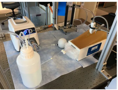
An ATS 700-D 527 calibrated flow phantom, manufactured by ATS Laboratories (Bridgeport, CT), was used in a setup to mimic blood flow through a small vessel. The rubber-based tissue mimic is calibrated for a sound velocity of 1,450 m/s with wave attenuation of 0.5 dB/cm/MHz at 23°C, as compared to a native soft tissue’s sound velocity of 1,540 m/s. However, rate of fluid flow is unaffected by this discrepancy. The vessel is 1 mm in diameter, and logVoA was measured for blood flow rates between 3.7 and 21.2 cm/s, with an accuracy of ± 0.2% in flow rate reading. Fluid flow was laminar for all measured flow rates.
The blood mimicking fluid used in this study was ATS 707-Doppler Test Fluid, with a viscosity of 1.66 ± 0.10 cSt and a density of 1.04 ± 0.01 g/cc, as measured at room temperature. The scatterer particles are 30 ± 3 µm in diameter, with a fluid concentration of 1.7 ±0.1 particles per cc. The flow pump was connected to the phantom using PVC tubing 10 mm in diameter, so the system was given adequate time to equilibrate and adjust to new flow rates over the course of the experiment.
Figure 1. Calibrated flow phantom experimental setup
ii. ARFI Imaging
In order to visualize the effects of blood flow rate on logVoA, data were acquired with and without an ARFI excitation using a Siemens Acuson Antares and VF7-3 linear array transducer in the calibrated flow phantom. The phantom was imaged both axially and laterally.
ARFI excitation pulses were generated at 300 cycles at 4.21 MHz, while tracking pulses were two cycles at 6.15 MHz at a focal depth of either 23 or 25 mm. The corresponding radio frequency (RF) data were used to measure ARFI-induced displacement with a normalized cross correlation procedure of kernel size 1.5λ [11], followed by two-stage interpolation and linear motion filtering [12, 13]. The acquired data was processing using MATLAB (Mathworks Inc., Natick, MA), and ARFI Peak Displacement (PDF) was calculated as the maximum displacement amplitude over time in each pixel, described in [11]. VoA was calculated as the variance of the second time derivative of displacement (i.e. acceleration) through time using the following equation,
(1))
V oA
(
x
, ,
y t
i=
N1−1∑
N t=1Acc
(
x
, , )
cc
(
x
, , )
|
|
|
|
y t
−
1
K
∑
t+K
tk=t
A
y t
k|
|
|
|
2
in which x and y represent the axial and lateral pixel coordinates, t is the time frame
Radio frequency SNR was derived as μ/σ, in which μ is the amplitude of the signal in each pixel per frame, while σ is the average signal amplitude in the anechoic region, representing the noise component of the signal [10].
Finally, each image was also processed using a Power Doppler algorithm as a point of comparison for the log VoA method. The MATLAB code used for analysis is included in the appendix, with annotations.
The contrast-to-noise ratio was calculated for logVoA, SNR, cross-correlation coefficient, and Power Doppler, using the equation,
CNR =
|μ −μ |
v b
(2)√
σ +σ
v2 2b
in which v and b represent the vessel and background regions, respectively, μ represents the logVoA parameter, and σ represents the variance in logVoA.
These vessel and background regions were determined by manual delineation on each B-mode image, using the ROIpoly function on MATLAB.
B. Preclinical in vivo Experiments
i. Animal protocol
The University of North Carolina at Chapel Hill Institutional Animal Care and Use Committee approved all animal experiments reviewed in this study. The aforementioned experiments included 2 male and 1 female pig with a mean body weight of 74.4 ± 9.3 kg at the time of study, and all pigs were anesthetized with telazol (2-3 mg/kg intramuscular) prior to procedure. The pigs were also administered atropine sulfate (0.03 mg/kg SQ) before endotracheal intubation to reduce pharyngeal secretion. Finally, the pigs were administered isoflurane (4-5%) via inhalation to induce anesthesia, which was maintained for the duration of the experiment. Intravenous fluid (0.9% NaCl) was infused at 5 mL/kg/hr, while an ear vein catheter introduced saline infusion at 5 mL/min. A pressure catheter (SPR-350S, Millar Inc., Houston, TX, USA) was placed in the femoral artery to monitor blood pressure using LabChart (ADinstruments, Colorado Springs, CO, USA). Pigs were prepped with an aseptic as instructed by the Division of Laboratory Animal Medicine guidelines, and the right kidney of each pig was exposed using laparotomy incisions. Finally, each kidney was excised with a combination of sharp and blunt dissection.
ii. ARFI Imaging
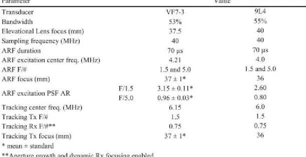
Table 1. ARFI imaging parameters using in in vivo experiment
The RF rata acquired during the experiment were transferred from the scanner to a computer for MATLAB (Mathworks Inc., Natick, MA) custom analysis. ARFI-induced displacement was calculated with a 1D axial normalized cross correlation [11] with the following parameters, described in [9]:
4X spline-based upsampling of RF data (natively sampled at 40 MHz), 376-μm kernel length (i.e. 1.5λ, in which λ represents the tracking pulse wavelength with a sound velocity of 1,540 m/s), and a search region of 80-μm. The normalized cross correlation-derived displacement versus time data was run through a quadratic filter to reduce motion artifacts [17]. The RF data was used to calculate the log compressed absolute value of the Hilbert-transformed RF data, which generated B-mode images. LogVoA was calculated as described for the phantom experiments.
Each kidney was imaged with ARFI in a baseline condition with normal blood flow in all renal vessels. The transducer was held in place during data acquisition using a stereotactic clamp. The transducer was placed along the kidney with the lateral field-of-view aligned across the direction of the nephrons in the cortex. Following this, each kidney was also imaged in an ischemic condition with the renal artery ligated to prevent blood flow into the kidney, with the same transducer orientation. ARFI data sets were acquired in immediate succession. [11]
LogVoA, ARFI PD, and Power Doppler were compared for differentiating between baseline and ischemic conditions, as well as in parametric 2D images for identifying small vessels in the kidney. The delineation mask was developed for automatically identifying small vessels based on a parametric threshold value and a filter for removal of independent pixels (code in appendix).
Figure 2 shows the B-mode, Power Doppler, and logVoA images of the CIRS phantom, imaged laterally, in which a 1 mm diameter vessel is indicated by the orange arrow. This vessel can be identified in the B-mode image, as well as the logVoA image. However, it cannot be visualized in the Power Doppler image. The vessel delineation was performed manually based on the B-mode image and was used for CNR calculations.
Figure 3 shows two plots of logVoA values along flow rates from 3.7 to 21.2 cm/s, when the phantom was imaged laterally. It can be observed that logVoA remains constant in the background, while it increases with flow rate in the vessel. Additionally, the ARFI push increases the values of logVoA for both vessel and background.
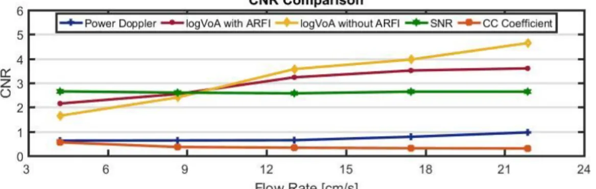
Figure 4 compares the contrast-to-noise ratio (CNR) in the vessel region of logVoA with and without ARFI, Power Doppler, SNR, and cross-correlation coefficient when imaged laterally. Of all the parameters shown, logVoA CNR increases the most with flow rate, both with and without ARFI.
Figure 5 shows the region of interest in the CIRS phantom when imaged in the axial configuration. The vessel is 1 mm in diameter, outlined in blue, and the background region is outlined in red.
Figure 6 shows two plots of logVoA values along flow rates from 0 to 53.05 cm/s, when the phantom is imaged axially. It can be observed that logVoA remains constant with flow rate in the background, while it increases in the vessel, similar to when the phantom is imaged laterally. Additionally, the ARFI push increases the values of logVoA in both the vessel and background.
Figure 7 shows two plots of Power Doppler values from 0 to 53.05 cm/s, when the phantom is imaged axially. Power Doppler performs well in this imaging configuration, as demonstrated in this experiment.
Figure 8 compares the contrast-to-noise ratio (CNR) in the vessel region of logVoA with and without ARFI, Power Doppler, SNR, and cross-correlation coefficient when imaged axially. Of all the parameters shown, logVoA CNR with ARFI excitation increases the most with flow rate. LogVoA CNR without ARFI does not have a consistent trend, while Power Doppler CNR decreases with flow rate.
Figure 9 compares logVoA across the cortex of all three pigs in the in vivostudy, for both the baseline and ischemic flow conditions. In all three pigs, logVoA is significantly lower in the ischemic case than baseline.
Figure 10 compares ARFI Peak Displacement across the cortex of all three pigs in the in vivostudy, for both the baseline and ischemic flow conditions. There is no significant difference in ARFI PD between the baseline and ischemic conditions in all three pigs.
Figure 11 compares Power Doppler across the cortex of all three pigs in the in vivostudy, for both the baseline and ischemic flow conditions. Trends in Power Doppler are inconsistent between the three pigs.
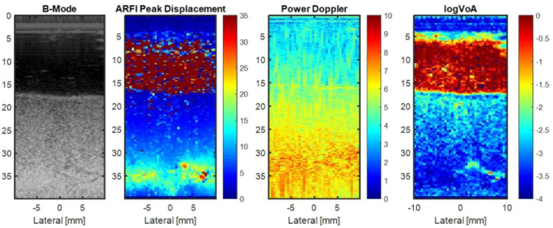
Figure 13 shows the delineation mask described in Methods applied to all the images in Figure 7, demonstrating that the vessel can only be identified clearly using the mask in the logVoA image.
Figure 2. Regions of interest in phantom, along with Power Doppler and logVoA images, imaged laterally
Figure 4. CNR in logVoA with and without ARFI, Power Doppler, SNR, and CC coefficient, imaged laterally
Figure 5. Region of interest in the phantom, imaged axially
Figure 7. Power Doppler vs. flow rate in vessel and background region of phantom, imaged axially
Figure 8. CNR in logVoA with and without ARFI, Power Doppler, SNR, and CC coefficient, imaged axially
A similar processing algorithm was used on the renal cortex in vivo data, and then log VoA was compared for the baseline and ischemic flow conditions.
Note: * indicates a significant difference between the two data sets.
Figure 10. ARFI PD compared in baseline vs. ischemic flow conditions in renal cortex
Figure 11. Power Doppler compared in baseline vs. ischemic flow conditions in renal cortex Note: * indicates a significant difference between the two data sets.
Figure 13. B-mode, ARFI Peak Displacement, Power Doppler, and logVoA images in renal cortex with artery ligated with delineation
IV. Discussion
The phantom was imaged both axially and laterally to evaluate logVoA and Power Doppler performance in both configurations. Regions of interest (ROIs) for the lateral configuration are delineated in figure 2. According to figure 3, logVoA increases with flow rate in the vessel region, while it stays relatively constant with flow rate in the background region when the phantom is imaged laterally. These results are as expected; logVoA should remain constant in the background region because SNR is constant over the course of the experiment and decorrelation caused by blood flow will not affect the phantom itself, only the lumen of the vessel, in which blood flow increases decorrelation. The threshold of flow rate detection using logVoA is approximately 9 cm/s, as labeled in figure 3 by the smallest detectable significant difference from 0 cm/s flow.
LogVoA in the vessel region increases with and without an ARFI excitation. In figure 4, the CNR of logVoA with and without an ARFI push is compared to Power Doppler CNR, and the results indicate a more marked increase in CNR with flow rate in the case with ARFI until a flow rate of 9 cm/s. This is due to the fact that the logVoA contrast between the background and vessel region is greater without an ARFI push than with an ARFI push at these flow rates. Power Doppler CNR shows a very small increase with flow rate, and the CNR remains below 1 until a flow rate of approximately 20 cm/s, confirming that Power Doppler’s performance is challenged in slow flow scenarios and small blood vessels.
(3)
in which decorrelation is denoted by ⍴, and an increase in both ⍴and SNR will lead to a higher calculated variance value (i.e. a higher logVoA). Frequency ( f), bandwidth (B) and tracking kernel (T) are all system parameters that are assumed to be held constant while imaging. As such, the logVoA results are driven by increase in decorrelation with flow rate in this experiment.
ROIs for the axial imaging configuration are delineated in figure 5. As per figure 6, when imaged axially, logVoA in the vessel region of the phantom increases with flow rate. This trend occurs both with and without an ARFI push, though the overall magnitude of change is greater with ARFI. LogVoA in the background region does not have a consistent trend with flow rate. Since SNR and decorrelation are not affected by direction of image acquisition, logVoA should perform well in both lateral and axial imaging constructs, as demonstrated in these results.
Power Doppler, on the other hand, performs much better when imaging axially than laterally. Figure 7 demonstrates that in an axial imaging configuration, Power Doppler in the vessel region increases with flow rate both with and without an ARFI push. Power Doppler in the background region does not have any consistent trend with flow rate. In this particular experiment, both Power Doppler and logVoA are adequate methods of assessing perfusion. However, in a lateral imaging construct, logVoA is advantageous over Power Doppler.
In figure 8, the results indicate that the increase in logVoA with flow rate is driven by decorrelation, similar to the results in the lateral imaging configuration. SNR CNR increases slightly with flow rate, which should actually cause logVoA to decrease, but the results show that logVoA actually increases. Cross-correlation coefficient CNR decreases with flow rate, and greater decorrelation leads to a higher logVoA, so this accounts for the increase in logVoA with flow rate. However, this only occurs with an ARFI push; without ARFI, logVoA CNR does not increase appreciably with flow rate. Additionally, Power Doppler CNR decreases with flow rate in figure 8. Since the actual Power Doppler signal increases with flow rate in this experiment, the decrease in CNR can be attributed to an increase in noise with higher fluid flow rates.
results. Additionally, the results show that neither ARFI PD nor Power Doppler are sufficient markers of perfusion in this experiment, validating the use of the logVoA parameter.
Additionally, in figure 12, B-mode, Power Doppler, ARFI PD, and logVoA were tested to identify a vessel. Figure 13 shows that the B-mode, ARFI PD, and Power Doppler images did not indicate any vessels or areas of high blood flow, but a logVoA-based mask delineated a small vessel in the renal cortex. These images were acquired with the artery ligated, which demonstrates that there was still some blood flow into the kidney even in the “ischemic” condition.
A limitation to the phantom study is that the vessel in the flow phantom was of a fixed diameter and could not be manipulated to test diameter effects on logVoA performance. As Power Doppler is successful in large vessels and high-flow scenarios, logVoA would also need to perform well in those cases to be clinically relevant as a parameter in measuring perfusion. Similarly, the blood mimicking fluid was held constant over the course of the experiment. Another experimental variable could have been variation in the amount of scatterers in the mixture over time to see how echogenicity affects logVoA association with blood flow.
One challenging aspect of the in vivo clinical study was that in some data sets, B-mode imaging did not clearly delineate the medulla and cortex regions of the kidney. To rectify this issue, the measurement ROIs were placed towards the outer edge of the kidney, but some ROIs may still have included portions of the medulla while imaging across the cortex. These two regions in the kidney differ in their mechanical properties [18], so this could be a source of error in the results. Another limitation is the small sample size of three pigs. Supplemental studies can include more experimental subjects and longer observation periods [9].
Future work can include developing a machine-learning algorithm to delineate features and/or vessels in a tissue in real time while imaging. In this study, the vessel shown in figures 12 and 13 was outlined using an automated segmentation algorithm developed manually. However, a software-based program could run a similar algorithm in real-time to allow for vessel detection during an experiment, allowing for immediate visualization of blood perfusion in a tissue. Additionally, the current segmentation algorithm utilizes the 2D logVoA image, but adding time vectors to the data set during an experiment could yield a more comprehensive segmentation.
The logVoA method can also be developed further. This study has demonstrated the use of logVoA as a marker to detect perfusion, but there are several variables involved in this that can be controlled and exploited in the future to find a quantitative association between logVoA and blood flow rate. The processing algorithm described in the Methods can also be applied to different imaging configurations with various transducer angles to see if logVoA performance can be maximized using a specific setup or orientation.
V. Conclusion
possible using a B-mode image, ARFI PD, or Power Doppler. Overall, the results suggest that the logVoA parameter is relevant to detecting tissue perfusion without the administration of contrast agents.
VI. Appendix
i. The code used to test Log VoA as a parameter for perfusion is shown below.
% Plot B-Mode
figure,imagesc(blat,baxial,bimage); colormap gray;
axis image; title('B-Mode')
% Plotting B-Mode image from ARFI frame: Isolate B-mode ROI
axial_i=knnsearch(baxial',axial(1)); axial_f=knnsearch(baxial',axial(end)); lat_i=knnsearch(blat',lat(1)); lat_f=knnsearch(blat',lat(end)); bimageROI=bimage(axial_i:axial_f,lat_i:lat_f); bimageROI=imresize(bimageROI,[length(axial) length(lat)]); bimageROI=medfilt2(bimageROI,[15 3]); figure,imagesc(lat,axial,bimageROI,[2.5 4.6]) colormap gray axis image
title('B-Mode Region of Interest')
hold on
contour(lat,axial,bac1,'r') contour(lat,axial,inc1,'b')
% Plot Peak displacement: apply Peak Displacement filter to ROI
figure,imagesc(lat,axial,Peak); colormap jet;
axis image;
title('Peak Displacement'); roipeak = Peak.*(roipolystat); roipeak(roipeak==0) = NaN; meanimage = nanmedian(roipeak(:)); meanstd = nanstd(roipeak(:)); set(gca,'clim',[0 10])
%lim = meanimage + meanstd; %set(gca,'clim',[0 lim])
% Plot Log Voa: apply Log VoA filter to ROI
lag=0;delay=5; clear frames
frames=zeros([size(acc,3)-delay+1 delay]);
for k=1:size(acc,3)
frames(k,:)=linspace(1+lag,delay+lag,delay);lag=lag+1; if (lag+delay)>size(acc,3), break, end
end
voaframes=zeros([size(acc,1) size(acc,2) size(frames,1)]); logvoaframes=zeros([size(acc,1) size(acc,2) size(frames,1)]);
for k=1:size(frames,1)
voaframes(:,:,k) = var(acc(:,:,frames(k,:)),[],3); logvoaframes(:,:,k) = log10(voaframes(:,:,k)); end
t2Dparam=medfilt2(squeeze(median(logvoaframes,3)),[15 3]);
ROI = zeros(size(Peak));
ROI(knnsearch(axial',30-10):knnsearch(axial',30),:)=1; Mask=t2Dparam.*ROI;
Mask(Mask==0)=NaN; Mask(Mask==Inf)=NaN; Mask(Mask==-Inf)=NaN;
range = [nanmedian(Mask(:))-nanstd(Mask(:)) nanmedian(Mask(:))+nanstd(Mask(:))];
figure,imagesc(lat,axial,t2Dparam,range); colormap jet; set(gca,'clim',[-3 1]); axis image; title('Log VoA') a2Dparam=squeeze(median(Peak,3));
ROI = zeros(size(Peak));
ROI(knnsearch(axial',30-10):knnsearch(axial',30),:)=1; Mask1=a2Dparam.*ROI;
Mask1(Mask1==0)=NaN; Mask1(Mask1==Inf)=NaN; Mask1(Mask1==-Inf)=NaN;
range1 = [0 nanmedian(Mask1(:))+nanstd(Mask1(:))];
%% Data Analysis: calculate displacement, acceleration, Log Voa, B-mode, and Power Doppler raw signal values over time in inclusion and background ROI
clear vector1 clear t1
%vector1 = arfidata; t1= t;
%vector1 = acc; t1 = t(1:size(acc,3));
%vector1 = bimageROI; t1 = t; %vector1 = CCcoeff; t1 = t;
clear dispHoletemp dispHole clear dispBacktemp dispBack for iii=1:size(vector1,3) % inclusion
dispHoletemp(:,:)=squeeze(vector1(:,:,iii)).*inc1; dispHole(iii,:)=reshape(dispHoletemp,[],1); end
dispHole(dispHole==0)=NaN; dispHole(dispHole==Inf) = NaN; dispHole(dispHole==-Inf) = NaN;
for iii=1:size(vector1,3) % background
dispBacktemp(:,:)=squeeze(vector1(:,:,iii)).*bac1; dispBack(iii,:)=reshape(dispBacktemp,[],1); end
dispBack(dispBack==0)=NaN; dispBack(dispBack==Inf) = NaN; dispBack(dispBack==-Inf) = NaN;
%% Statistics: calculate median and standard deviation of raw signal values in inclusion and background
med1 = nanmedian(dispHole'); sd1 = nanstd(dispHole') sdlow1 = med1-sd1 sdhigh1 = med1+sd1
med2 = nanmedian(dispBack') sd2 = nanstd(dispBack') sdlow2 = med2-sd2 sdhigh2 = med2+sd2
%% Contrast to Noise Ratio (CNR): calculate CNR of inclusion and background regions
mu_back = nanmean(dispBack'); mu_hole = nanmean(dispHole'); stand1 = sd1.^2;
stand2 = sd2.^2;
mu_back_hole = abs(mu_hole - mu_back); stands_back_hole = sqrt(stand1 + stand2);
CNR_back_hole = mu_back_hole./stands_back_hole;
ii. The code implemented to develop a mask using threshold-based segmentation and a filter removing independent pixels for the in vivo study is shown below.
figure,imagesc(lat,axial,t2Dparam)
mask=zeros(size(t2Dparam,1),size(t2Dparam,2)); % mask(medfilt2(t2Dparam,[10 3])>-2.7)=1; % mask(t2Dparam>20)=1; %Peak
% mask(t2Dparam>7.1)=1; %power doppler % mask(t2Dparam<4)=1; %bmode
mask(t2Dparam>-2.7)=1;
%% Filter removing independent pixels from mask
mask2 = bwareaopen(mask, 100);
% mask2 = bwareaopen(medfilt2(mask,[20 3]), 100); mask2(1:knnsearch(axial',29),:)=0;
figure,imagesc(lat,axial,mask)
figure,imagesc(lat,axial,medfilt2(mask,[20 3])) figure,imagesc(lat,axial,mask2)
figure,imagesc(lat,axial,t2Dparam,[-3 0]) hold on
VII. References
1. Frohlich ED, Quinlan PJ. Coronary heart disease risk factors: public impact of initial and later-announced risks. Ochsner J. 2014;14(4):532–537.
2. Pinter SZ, Lacefield JC. Detectability of small blood vessels with high-frequency power Doppler and selection of wall filter cut-off velocity for microvascular imaging. Ultrasound
Med Biol 2009; 35:1217–1228.
3. Xu, Tiantian, et al. “In Vivo Lateral Blood Flow Velocity Measurement Using Speckle Size Estimation.” Ultrasound in Medicine & Biology, vol. 40, no. 5, May 2014, pp. 931–937., doi:10.1016/j.ultrasmedbio.2013.11.017.
4. Calliada, F, et al. “Ultrasound Contrast Agents.” European Journal of Radiology, vol. 41, no. 3, May 2002, p. 175., doi:10.1016/s0720-048x(02)00022-0.
5. Pasternak JJ, Williamson EE. Clinical pharmacology, uses, and adverse reactions of iodinated contrast agents: a primer for the non-radiologist. Mayo Clin Proc.
2012;87(4):390-402.
6. Geist, Rebecca E., et al. “Experimental Validation of ARFI Surveillance of Subcutaneous Hemorrhage (ASSH) Using Calibrated Infusions in a Tissue-Mimicking Model and Dogs.”
Ultrasonic Imaging, vol. 38, no. 5, 27 Nov. 2015, pp. 346–358.,
doi:10.1177/0161734615617940.
7. Omari, E.A., and Varghese, T. “Signal to Noise Ratio Comparisons for Ultrasound
Attenuation Slope Estimation Algorithms.” Medical Physics, vol. 41, no. 3, 3 Mar. 2014.NCBI, doi:10.1118/1.4865781.
8. Torres, Gabriela, et al. “In Vivo Delineation of Human Carotid Plaque Features with ARFI Variance of Acceleration (VoA).” 2017 IEEE International Ultrasonics Symposium (IUS), 2017, doi:10.1109/ultsym.2017.8091836.
9. Hossain, Md Murad, et al. “Mechanical Anisotropy Assessment in Kidney Cortex Using ARFI Peak Displacement: Preclinical Validation and Pilot In Vivo Clinical Results in Kidney Allografts.” IEEE Transactions on Ultrasonics, Ferroelectrics, and Frequency Control, vol. 66, no. 3, Mar. 2019, pp. 551–562., doi:10.1109/tuffc.2018.2865203.
10. Torres, Gabriela, et al. “In Vivo Delineation of Human Carotid Plaque Features with ARFI Variance of Acceleration (VoA).” 2017 IEEE International Ultrasonics Symposium (IUS), Mar. 2019, doi:10.1109/ultsym.2017.8091836.
11. G.F. Pinton, J.J. Dahl, G.E. Trahey. “Rapid tracking of small displacements with ultrasound.”
IEEE Trans Ultrason Ferroelectr Freq Control, 53 (2006), pp. 1103-1117
12. K. Nightingale, M.S. Soo, R. Nightingale, G. Trahey. “Acoustic radiation force impulse imaging: in vivo demonstration of clinical feasibility.” Ultrasound Med Biol, 28 (2002), pp. 227-235
13. B.J. Fahey, M.L. Palmeri, G.E. Trahey. “The impact of physiological motion on tissue tracking during radiation force imaging.” Ultrasound Med Biol, 33 (2007), pp. 1149-1166 14. Preston, Richard A., and Murray Epstein. “Ischemic Renal Disease.” Journal of
Hypertension, vol. 15, no. 12, 1997, pp. 1365–1377.,
doi:10.1097/00004872-199715120-00001.
15. Correas J-M, Bridal L, Lesavre A, Méjean A, Claudon M, Hélénon O. Ultrasound contrast
agents: properties, principles of action, tolerance, and artifacts. European Radiology.
2001;11(8):1316-1328. doi:10.1007/s003300100940.
16. Lorusso A, Quaia E, Poillucci G, Stacul F, Grisi G, Cova MA. Activity-based cost analysis of contrast-enhanced ultrasonography (CEUS) related to the diagnostic impact in focal liver
lesion characterisation. Insights into Imaging. 2015;6(4):499-508.
17. R. H. Behler, T. C. Nichols, E. P. Merricks, and C. M. Gallippi, “A rigid wall approach to physiologic motion rejection in arterial radiation force imaging,” in Proc. IEEE Ultrason. Symp., Oct. 2007, pp. 359–364.
18. J.-L. Gennisson, N. Grenier, C. Combe, and M. Tanter, “Supersonic shear wave elastography of in
vivo pig kidney: Influence of blood pressure, urinary pressure and tissue anisotropy,” Ultrasound