Vol. 19, No. 01, pp 163-183 DOI:10.29252/jirss.19.1.163
Parameter Estimation of Some Archimedean Copulas Based on
Minimum Cramér-von-Mises Distance
Selim Orhun Susam1
1Department of Econometrics, Munzur University, Turkey.
Received: 31/01/2019, Revision received: 02/08/2019, Published online: 26/08/2019
Abstract. The purpose of this paper is to introduce a new estimation method for estimating the Archimedean copula dependence parameter in the non-parametric setting. The estimation of the dependence parameter has been selected as the value that minimizes the Cramér-von-Mises distance which measures the distance between Empirical Bernstein Kendall distribution function and true Kendall distribution function. A Monte Carlo study is performed to measure the performance of the new estimator and compared to conventional estimation methods. In terms of estimation performance, simulation results show that the proposed Minumum Cramér-von-Mises estimation method has a good performance for low dependence and a small sample size when compared with the other estimation methods. The new minimum distance estimation of the dependence parameter is applied to model the dependence of two real data sets. Keywords.Cramér-von-Mises, Archimedean Copula, Parameter Estimation, Bernstein Polynomials
MSC:62G05, 62G32
Corresponding Author: Selim Orhun Susam ([email protected])
1
Introduction
Copula models are popular tools for describing the dependency of multivariate data where the univariate distribution functions are combined with joint distribution function by Sklar’s theorem (Sklar (1959)). Consider random variables X and Y with joint cumulative distribution functionH and marginalsF andG, respectively. Then there exist a copulaCsuch thatH(x,y)=C(F(x),G(y)), for allx,yin<.
An important family of the copula is known as Archimedean copula. This copula class is characterized by generator function ϕ. In application, ϕ belongs to the parametric familyϕθfor which the parameterθneeds to be estimated. This paper aims to investigate the estimation of parameterθand to present a Monte Carlo simulation study on the performance of proposed estimators for some Archimedean copulas. For three popular parametric Archimedean copulas, classical maximum likelihood and inversion of Kendall’s tau estimators are compared with the minimum Cramér-von-Mises estimator.
In the literature, there are many studies for estimating the dependency parameter. Deheuvels (1978), Genest et al. (1995), Joe (1996), Joe (1997), Joe (2005), Fermanian et al. (2004), Kim et al. (2007), Najafabadi et al. (2013), Biau et al. (1985), Tsukahara (2005), Mendes et al. (2007) and Weib (2011) studied the estimation methods and gave some comparisons among them. This paper is closely related to the works of Tsukahara (2005), Mendes et al. (2007), Biau et al. (1985) and Weib (2011). The similarity with these articles is the usage of the minimum distance method in parameter estimation. Tsukahara (2005) investigated the limiting behavior of the empirical copula process and applied it to prove some asymptotic properties of a minimum distance estimator for an Euclidean parameter in a copula model. Mendes et al. (2007) obtained robust estimators for copula parameters through the minimization of weighted goodness-of-fit statistics. Biau et al. (1985) introduced a minimum L1 distance estimate for parametric copula
densities. Weib (2011) presented a comprehensive Monte Carlo simulation study on the performance of minimum-distance and maximum-likelihood estimators for bivariate parametric copulas. In particular, they considered Cramér-von-Mises, Kolmogorov-Smirnov andL1-variants of the CvM-statistic based on the empirical copula process,
Kendall’s dependence function and Rosenblatt’s probability integral transform. The dissimilarity of this study from other minimum distance estimation methods is the usage of Bernstein polynomials for estimation of Kendall distribution function.
The remainder of the study is organized as follows. In Section 2, we give the general concept of Archimedean copulas and their properties. Also, we review the estimation
methods of the dependence parameter, and in addition to the new flexible estimation method, the dependence parameter of Archimedean copula is introduced. In section 3, the estimation results of Monte Carlo simulation are given. Section 4 is devoted to real data applications. Lastly, the final section is devoted to the conclusion.
2
Archimedean Copulas
Archimedean copula models form a useful family of copula models in which the dependence structure can be characterized by a univariate distribution function (Nelsen (2006), Section 4). One of their important features that separates this class from the others is that it has a generator functionϕwhich is used to construct an Archimedean copula. Archimedean copula with generator functionϕ,C : [0,1]2 →[0,1] is defined by
C(u,v)=ϕ[−1]{ϕ(u)+ϕ(v)}; u,v∈[0,1].
This generator function and its pseudo-inverse function are defined in Nelsen (2006) by the following definition,
Definition 2.1. A generator functionϕis a continuous, strictly decreasing convex function defined from [0,1] to [0,∞) such thatϕ(1)=0. Ifϕ(0)=∞, then the generator is called as a strict generator. The pseudo inverse ofϕis the functionϕ[−1], defined on [0,∞) to [0,1] is given by
ϕ[−1]
= (
ϕ−1
(t) 0≤t≤ϕ(0) 0 ϕ(0)≤t<∞.
An Archimedean copula can be reduced to a univariate distribution function through generator function. Genest et al. (1993) showed that the function ϕcan be obtained by the univariate distribution functionK(t) =P(C(u,v) ≤t) Remarkably, there is a link between the functionϕandK(t) such as
K(t)=t− ϕ(t)
ϕ0
(t) t∈(0,1).
K(t), called as Kendall distribution function, identifies the generator functionϕ(t) and so the dependence structure of the Archimedean copula family. In Table 1, some Archimedean copulas with a generator function and Kendall distribution function are summarized.
Table 1: Archimedean copulas with generator function.
Copula ϕ(t) K(t) τ(θ) Range ofθ
Clayton (t−θ−
1)/θ t+t(1−θtθ) θθ+2 (−1,∞)− {0} Frank −log(exp(tθ)−1
exp(θ)−1) t−
(exp(tθ)−1)log(expexp((−−tθθ))−−11)
θ 1+4θ
−1
(D1*(θ)−1) (−∞,∞)− {0} Gumbel (−log(t))θ t−tlog(t)
θ θ
−1
θ [1,∞)
Independence −log(t) t−tlog(t) -
-*D
1is the first Debye function of order 1,D1(x)=x−1 Rx
0 t(exp(t)−1) −1dt
Genest et al. (1993) proposed a nonparametric procedure using an empirical estimate ˆ
Kn of K. Let (X1,Y1),(X2,Y2), . . . ,(Xn,Yn) be a random sample of size n from a pair (X,Y) with the copula C. For i = 1, . . . ,n, consider the psuedo observations
Ti = Pnj=1I(Xi < Xj,Yi < Yj)/(n−1). The Kendall distribution function, K(t) is then estimated by the empirical distribution function
Kn(t)= n
X
i=1
I(Ti≤t)/n.
Susam et al. (2018) defined the Bernstein estimator of order (m > 0) of the Kendall distribution function K as,
Km,n(t)= m
X
k=0
Kn(k/m)Pk,m(t),
where Pk,m(t) = mktk(1−t)m−k is the Binomial probability and Kn is the empirical distribution function ofK(t). They conclude that Bernstein Kendall estimator outperms the classical Kendall estimator. Because, Bernstein Kendall estimator is flexible with regard to its polynomial degree.
2.1 Parameter Estimation via Inversion of Kendall’s Tau
IfCis a bivariate Archimedean copula with generator functionϕ, Genest et al. (1986) defined Kendall’s tau as
τ=1+4 Z 1
0 ϕ(t)
ϕ0 (t)dt,
which can be computed for some Archimedean copulas, see Table 1. Genest et al. (1993) introduce a method-of-moments estimator for bivariate one-parameter Archimedean copulas based on Kendall’s tau. Let τ = h(θ) be the Kendall’s tau and let τn be the empirical Kendall’s tau based on a random sample of size n. Then the moment estimator ofθdenoted by ˆθis given by ˆθ=h−1(τ
n),τn =4 ¯T−1, where, ¯T= 1nPni=1Ti.
h(θ) function is also listed in Table 1. √
n( ˆθ−θ) is asymptotically normal with zero mean. (See, Kojadinovic et al. (2010)).
2.2 Maximum-Likelihood Estimation of Parameter
The most popular method for estimating the dependence parameter θ is based on Maxiumum Likelihood principle. This method is applicable for all absolute continuous copula classes. Suppose that copulaC(u,v) has a densityc(u,v) defined by
c(u,v)= ∂
2C(u,v)
∂u∂v u,v∈(0,1).
When the marginsFandGare known, the log-likelihood function forθis defined as
l(θ)= n
X
i=1
log(c(F(xi),G(yi))).
Oakes (1994) proposed to replaceF(x),G(y) with their empirical counterpartsFn(x) and
Gn(y), respectively. Genest et al. (1995) defined empirical estimates of marginals as
Fn(x)= 1
n+1 n
X
i=1
I(Xi≤x), Gn(y)= 1
n+1 n
X
i=1
I(Yi ≤y),
whereI denotes indicator function. Then, Log-maximum psuedo likelihood function
l∗(θ) is given by
l∗(θ)= n
X
i=1
log(c(ui,vi)),
whereui= rankn+(X1i)andvi= rankn+(1Yi). The maximum likelihood estimator is the value ˆθMLEn that maximizesl∗(θ). Genest et al. (1995) showed that ˆθMLEn is a consistent estimator.
2.3 Minumum Cramér-von-Mises Estimator Based on Kendall Distribution Function
Let K(t) be Kendall distribution function associated with copula C and let Kn(t) be the empirical Kendall distribution function. The Cramér-von-Mises (CvM) distance betweenK(t) andKn(t) is defined by
CvM=
Z 1
0
Kn(t)−K(t)
2
dt.
The estimation of the dependence parameter θ can be selected as the value that minimizes the CvM function. Weib (2011) proposed estimation methods of Archimedean copula dependence parameter using Cramér-von-Mises distance. They used classical Empirical estimation methods of Kendall distribution function in the estimation of the dependence parameter. In contrast to Weib (2011), we use the Bernstein Empirical estimation of Kendall distribution function instead of the classical empirical estimation. CvM distances for Bernstein estimation of Kendall distribution function for Gumbel, Clayton and Frank copulas are defined in next Lemma.
Lemma 2.1. Let KGu(t), KCl(t) and KFr(t) be Kendall distributions of the Gumbel, Clayton
and Frank copulas and let Km,n(t)be the Bernstein estimator of Kendall’s distribution function.
The Cramer-von-Mises (CvM) distances between Km,n(t)and KGu(t), KCl(t), KFr(t), denoted
by CvMGu, CvMCl, CvMFrare given by
CvMGu= m
X
k=0 m
k
!2
K2n(k
m)Beta(2k+1,2m−2k+1)
+2 m−1 X
k=0
m
X
s=k+1 m
k
!
m s
!
Kn(
k m) ˆKn(
s
m)Beta(k+s+1,2m−k−s+1)
−2 m
X
k=0
m k
!
Kn(k
m)
Beta(k+2,m−k+1)− m−k X
i=0
(−1)i
θ
m−k
i
!
(− 1
(k+i+2)2)
!
+2+6θ+9θ2
27θ2 .
CvMCl= m X k=0 m k !2
K2n(k
m)Beta(2k+1,2m−2k+1)
+2 m−1 X k=0 m X s=k+1 m k ! m s !
Kn(
k m)Kn(
s
m)Beta(k+s+1,2m−k−s+1)
−2 m X k=0 m k !
Kn(k
m)
Beta(k+2,m−k+1)(θ+1
θ )−
β(k+θ+2,m−k+1)
θ
!
+ 17+13θ+2θ2
27(1+θ)+6θ2.
CvMFr = m X k=0 m k !2
K2n(k
m)Beta(2k+1,2m−2k+1)
+2 m−1 X k=0 m X s=k+1 m k ! m s !
Kn(k
m)Kn( s
m)Beta(k+s+1,2m−k−s+1)
−2 m
X
k=0
m k
!
Kn(
k m)
Beta(k+2,m−k+1)− m−k X
i=0
(−1)i
θ
m−k
i
!
A(t,k,i) !
+B(t, θ),
where A(t,k,j)and B(t, θ)are numerical solutions of theR01tk+j(exp(t∗θ)−1) log(exp(−tθ)−1
exp(−θ)−1)
andR1 0
t−(exp(tθ)−1)
θ log(exp(
−tθ)−1
exp(−θ)−1) 2
dt respectively. See the appendix for detailed calculations.
Then minimum Cramér-von-Mises estimation of parameterθfor Gumbel, Clayton and Frank copulas are defined as
ˆ
θCvM
n,m =argmin
θ∈Θ n
CvM(∗) o
,
where m denotes the degree of the Bernstein polynomial and also this non-linear optimization problem can easily be solved by Statistical programming language R or Mathematica.
From Leblanc (2012) and Susam et al. (2018), we know that ˆKm,n(t) is a consistent estimator. Also, Duchesne et al. (1997) show that ˆθCvM
n is a consistent estimator.
3
Simulation Study
Monte Carlo simulation study was conducted to compare Inversion of Kendall’s tau estimator, Maximum likelihood estimator and Minumum Cramér-von-Mises estimator of dependence parameterθof Gumbel, Clayton, Frank copulas, and to asses estimated MSE’s of estimations. The primary purpose is achieved by comparing the true parameter with the parameters estimated with the three estimation methods. The data are generated from three Archimedean copulas such as Clayton. Gumbel, and Frank with Kendall’s Tau 0.1, 0.2,...,0.8. These distributions cover different shapes and characteristics. The Clayton copula exhibits strong left tail dependence. Gumbel copula cannot model negative dependence, but it contrasts to Clayton, Gumbel has strong right tail dependence. Moreover, Frank copula exhibits symmetric and weak tail dependence in both tails. 10,000 Monte Carlo samples of sizesn=75 and 150 are generated from each type of Archimedean copulas. All computations were performed in R. We used the package "copula" for generating the data. Also, “nloptr” package was used for solving non-linear equations.
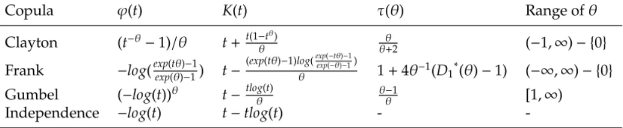
Table 2: Estimated MSE’s scores of Gumbel copula parameter estimators for sample size n=75.
τ θˆτ
n θˆMLEn θˆCvMn,m=10 θˆCvMn,m=20 θˆCvMn,m=30
0.1 0.0089 0.0096 0.0239 0.0116 0.0081 0.2 0.0159 0.0171 0.0320 0.0191 0.0114 0.3 0.0255 0.0282 0.0452 0.0287 0.0245 0.4 0.0407 0.0426 0.0639 0.0429 0.0375 0.5 0.0696 0.0706 0.0949 0.0697 0.0622 0.6 0.1229 0.1129 0.1450 0.1149 0.1094 0.7 0.2544 0.2162 0.2411 0.2229 0.2145 0.8 0.5999 0.4525 0.5154 0.5096 0.5848
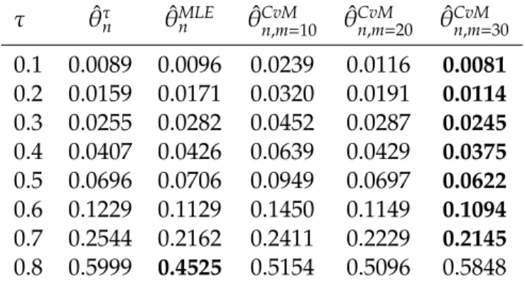
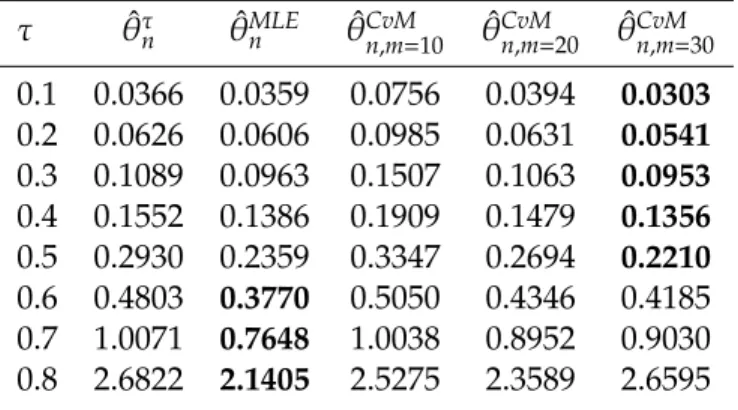
The results given in Tables 2-7 show that, as expected, estimated MSE’s of parameter estimation of all Archimedean copulas decrease as sample size increases. This is required by the consistency of the Bernstein estimate of Kendall distribution function. On the other hand, estimated MSE’s scores increase with increasing Kendall’s tau for all Archimedean copulas and estimation methods. For sample size 75, Minimum Mises estimator outperforms other estimation methods. Minimum Cramér-von-Mises performed better than others due to its flexibility since by increasing polynomial
degree estimated MSE’s scores can be decreased for Minimum Cramér-von-Mises estimator. For sample size 150, the Maximum Likelihood estimator outperforms the other estimators.
Table 3: Estimated MSE’s scores of Gumbel copula parameter estimators for sample size n=150.
τ θˆτ
n θˆMLEn θˆCvMn,m=10 θˆCvMn,m=20 θˆCvMn,m=30
0.1 0.0041 0.0044 0.0170 0.0068 0.0068 0.2 0.0071 0.0074 0.0234 0.0107 0.0079 0.3 0.0118 0.0117 0.0316 0.0159 0.0124 0.4 0.0188 0.0181 0.0450 0.0243 0.0193 0.5 0.0311 0.0281 0.0628 0.0375 0.0313 0.6 0.0577 0.0511 0.0945 0.0641 0.0575 0.7 0.1121 0.0945 0.1555 0.1158 0.1125 0.8 0.2706 0.2226 0.2859 0.2627 0.3144
Table 4: Estimated MSE’s scores of Clayton copula parameter estimators for sample size n=75.
τ θˆτ
n θˆMLEn θˆCvMn,m=10 θˆCvMn,m=20 θˆCvMn,m=30
0.1 0.0366 0.0359 0.0756 0.0394 0.0303 0.2 0.0626 0.0606 0.0985 0.0631 0.0541 0.3 0.1089 0.0963 0.1507 0.1063 0.0953 0.4 0.1552 0.1386 0.1909 0.1479 0.1356 0.5 0.2930 0.2359 0.3347 0.2694 0.2210 0.6 0.4803 0.3770 0.5050 0.4346 0.4185 0.7 1.0071 0.7648 1.0038 0.8952 0.9030 0.8 2.6822 2.1405 2.5275 2.3589 2.6595
4
Real Data Examples
To demonstrate the new estimation methods presented in the previous sections, we fit the Gumbel, Clayton and Frank copula to the following two real data sets in this
section:
1. According to the manual of R’s package “MASS”, the US National Institute of Diabetes and Digestive and Kidney Diseases collected a data set from the population of women (at least 21 years old, of Pima Indian heritage and living near Phoenix, Arizona) who were tested for diabetes according to World Health Organization criteria. The data set “Pima.tr” contains a randomly selected set of 200 subjects.
2. According to the manual of R’s package “boot”, the excess return for the Acme Cleveland Corporation are recorded along with those for all stocks listed on the New York and American Stock Exchanges recorded over five years. These excess returns are relative to the return on a risk-less investment such a U.S. Treasury bills. The data set contains 60 samples of each variable.
Table 5: Estimated MSE’s scores of Clayton copula parameter estimators for sample size n=150.
τ θˆτ
n θˆMLEn θˆCvMn,m=10 θˆCvMn,m=20 θˆCvMn,m=30
0.1 0.0167 0.0154 0.0555 0.0227 0.0138 0.2 0.0292 0.0261 0.0667 0.0337 0.0231 0.3 0.0454 0.0385 0.0914 0.0526 0.0427 0.4 0.0780 0.0602 0.1266 0.0842 0.0727 0.5 0.1263 0.1007 0.1937 0.1362 0.1193 0.6 0.2491 0.1946 0.3437 0.2592 0.2325 0.7 0.5183 0.3960 0.6444 0.5206 0.4881 0.8 1.3206 1.0284 1.4690 1.2783 1.3155
The scatterplots of the data sets are shown in Figure 1. In Figure 1, it is observed that there is a visible dependence structure of two data sets. Kendall’s tau was measured as 0.1842 for variables between body mass index and dialectic blood pressure for Pima Indian womens, and as 0.3649 for variables between the excess return of the market and excess return for the Acme Corporation.
We apply goodness of fit testing procedure based on parameter estimations methods introduced in section 2. Genest et al. (2008) proposed a test statistic for testing the null
Table 6: Estimated MSE’s scores of Frank copula parameter estimators for sample size n=75.
τ θˆτ
n θˆMLEn θˆCvMn,m=10 θˆCvMn,m=20 θˆCvMn,m=30 0.1 0.5478 0.5592 0.8052 0.4417 0.4710 0.2 0.5675 0.5733 0.8467 0.5171 0.5673 0.3 0.6827 0.6820 0.9449 0.6246 0.6799 0.4 0.7618 0.7412 0.9538 0.6707 0.7217 0.5 1.0855 1.0342 1.2285 0.9217 1.0109 0.6 1.5555 1.4228 1.5745 1.3810 1.3867 0.7 2.6039 2.2988 2.4870 2.2182 2.8495 0.8 6.1027 5.1382 6.7891 11.0283 8.0771
Table 7: Estimated MSE’s scores of Frank copula parameter estimators for sample size n=150.
τ θˆτ
n θˆMLEn θˆCvMn,m=10 θˆCvMn,m=20 θˆCvMn,m=30
0.1 0.2527 0.2572 0.6133 0.3513 0.2980 0.2 0.2859 0.2848 0.6319 0.3713 0.3298 0.3 0.3269 0.3225 0.6242 0.3887 0.3591 0.4 0.3931 0.3822 0.6660 0.4385 0.4156 0.5 0.5323 0.5214 0.8532 0.5749 0.5612 0.6 0.7310 0.6899 0.9752 0.7162 0.7217 0.7 1.2181 1.1520 1.5066 1.1826 1.1914 0.8 2.6545 2.3927 3.0553 3.2469 4.2071
hypothesisH0:K(t)=Kθˆ(t) as CvM=
Z 1
0
nKn(t)−Kθˆ(t)
2
dKθˆ(t),
P-values are obtained by parametric bootstrap method as described in Genest et al. (2008).
Estimations and Goodness of fit results for two data sets presented in Tables 8, 9. When Table 8 is examined, it is seen that CvM measure and associated P-values have approximately the same values in almost all cases. Despite this, CvM measure based
on minimum distance estimator is slightly lower than the other estimation methods. These results are similar to the results obtained by Monte Carlo simulations for a small sample size and τ = 0.4 in section 3. In Table 9, small CvM measures are obtained for minimum distance estimators with polynomial degree m = 30. Unlike simulation results for big sample size and τ = 0.2, minimum distance estimator has lower CvM measure than the others. Also, we note that CvM measure decreases with increasing polynomial degree for minimum distance estimator for two data sets. Also, Figures 2-3 visualizes the fit on the empirical λfunction. In Figures 2-3, empiricalλ functions are presented by solid lines and parametric estimation of λfunctions with parameters estimated by minimum distance estimator are presented by dashed lines. Three parametric estimation ofλfunctions are presented in Figures 2-3. We estimated Clayton and Frankλ function’s parameters using minimum distance estimator with Bernstein polynomial degreem=10,20,30 for the two data sets. Estimated parameters are given in Tables 8-9. We preferred λ functions as a visual comparison on the goodness of fit performance for two real data sets; because λ(t) = ϕϕ0((tt)) function is visually more informative than the Archimedean generatorϕand Kendall distribution
K. For more details about λ function, see Michiels et al. (2012). From Figures 2-3, when the polynomial degreemincreases, parametric estimation of Clayton and Frank
λfunctions get closer to the empiricalλfunction of the two data sets.
−0.25 −0.20 −0.15 −0.10 −0.05 0.00 0.05
−0.3
−0.2
−0.1
0.0
0.1
0.2
The excess return of the market as a whole
The e
xcess retur
n f
or the Acme Cor
por
ation
(a) Data set for Excess returns.
40 50 60 70 80 90 100 110
20
25
30
35
40
45
Body mass index
Diastolic b
lood pressure
(b) Data set for Pima Indian Womens.
Figure 1: Scatter plots of the data sets.
Table 8: Estimation and goodness of fit results for excess return for the Acme Cleveland. Copula θˆτn θˆMLEn θˆCvMn,m=10 θˆCvMn,m=20 θˆCvMn,m=30
Gumbel Estimation 1.5747 1.5515 1.8118 1.6860 1.6731
CvM 0.1714 0.1799 0.1365 0.1456 0.1470
P-Value 0.0253 0.0172 0.0282 0.0328 0.0331
Clayton Estimation 1.1494 1.3519 1.4678 1.2492 1.2303
CvM 0.0463 0.0529 0.0642 0.0472 0.0417
P-Value 0.7401 0.6320 0.4171 0.6286 0.7682
Frank Estimation 3.6969 3.7978 4.4861 3.9375 3.9091
CvM 0.1391 0.1361 0.1333 0.1332 0.1331
P-Value 0.0415 0.0525 0.0373 0.0315 0.0561
Table 9: Estimation and goodness of fit results for Pima Indian Womens. Copula θˆτn θˆMLEn θˆCvMn,m=10 θˆCvMn,m=20 θˆCvMn,m=30
Gumbel Estimation 1.2258 1.1607 1.3064 1.2231 1.1953
CvM 0.0602 0.0685 0.1261 0.0593 0.0559
P-Value 0.4714 0.4971 0.4981 0.6535 0.6286
Clayton Estimation 0.4517 0.3400 0.5576 0.4055 0.3489
CvM 0.1517 0.0768 0.2776 0.1113 0.0730
P-Value 0.0754 0.3145 0.0371 0.2031 0.3525
Frank Estimation 1.7055 1.6517 2.0886 1.6083 1.5139
CvM 0.0618 0.0548 0.1415 0.0501 0.0422
P-Value 0.4334 0.5322 0.3651 0.8121 0.8020
5
Concluding Comments
In this study, we propose a method of estimating the parameter for some bivariate Archimedean copula. We estimate the dependence parameter using Cramér-von-Mises distance and Bernstein polynomial approximation. We also use the MSE values to measure the performance of the estimators. Our simulation suggests that the Minumum Cramér-von-Mises estimation method has a good performance for low dependence and small sample size when compared with the other estimation methods.
0.0 0.2 0.4 0.6 0.8 1.0
−0.30
−0.25
−0.20
−0.15
−0.10
−0.05
0.00
t
λ
(
t
)
Empirical Lambda λCl(t, θ^n, m=10) λCl
(
t, θ^n, m=20)
λCl
(
t, θ^n, m=30)
Figure 2: Empiricalλand parametric estimation of Claytonλfunctions with parameter obtained by minimum distance estimator for the Acme Cleveland Corporation data set.
0.0 0.2 0.4 0.6 0.8 1.0
−0.35
−0.25
−0.15
−0.05
0.00
t
λ
(
t
)
Empirical Lambda
λFr
(
t, θ^n, m=10)
λFr(
t, θ^n, m=20)
λFr(
t, θ^n, m=30)
Figure 3: Empiricalλand parametric estimation of Frankλfunctions with parameter obtained by minimum distance estimator for the Pima Indian woman data set.
However, this result is no longer valid at higher Kendal’s tau values. We established estimations and Goodness of fit results for two data sets. CvM measure based on the minimum distance estimator is slightly lower than the other estimation methods for a small sample size. Unlike simulation results for big sample size, minimum distance estimator has lower CvM measure than the others. In practice, weight selection is important for specific types of dependence. For example, Clayton copula has a heavy concentration of probability near (0,0). On the contrary, Gumbel copula has a heavy concentration of probability near (1,1). Also, Frank copula exhibits symmetric dependence. If one can propose a method, which minimizes “weighted” Cramér-von-Mises distance according to the dependence structure of data, it should most probably decrease estimated MSE’s scores.
Acknowledgments
We thank the anonymous referees and the editor for their helpful suggestions which improved the presentation of the paper.
References
Biau, G., and Wegkamp, M. (2005), Minimum distance estimation of copula densities.
Statistics & Probability letters,73, 105–114.
Deheuvels, P. (1978), Caracterisation complete des lois extremes multivariees et de la convergence des types extremes.Publications de lInstitut de Statistique de lUniversite de Paris,3, 1–36.
Duchesne, T., Rioux, J., and Luong, A. (1997), Minimum Cramér-von Mises distance methods for complete and grouped data. Communications in statistics-theory and methods,26, 401–420.
Fermanian, J. D., Radulovic, D., and Wegkamp, M. (2004), Weak convergence of empirical copulaprocesses.Bernoulli,10, 847–860.
Genest, C., and Mackay, R. J. (1986), Copules archimediennes et families de lois bidimensionelles dont les marges sont donnees. Canadian journal of statistics, 14, 145–159.
Genest, C., and Rivest, L. (1993), Statistical inference procedures for bivariate archimedean copulas.Journal of the American Statistical Association,88, 1034–1043.
Genest, C., Molina, J., and Lallena, J. (1995), De l’impossibilite de construire des lois a marges multidimensionnelles donnees a partir de copules. Comptes rendus de l’Acadmie des Sciences,320, 723–726.
Genest, C., Rémillard, B., and Beaudoin, D. (2008), Goodness-of-fit tests for copulas: A review and a power study.Insurance: Mathematics and Economics,44, 199–213. Joe, H. (1978), Asymptotic efficiency of the two-stage estimation method for
copula-based models.Journal of Multivariate Analysis,94, 401–419.
Joe, H., and Xu, J. (1996), The estimation method of inference functions for margins for multivariate models.Technical Report,166, The University of British Columbia. Joe, H. (1997),Multivariate Models and Dependence Concepts.London, England: Chapman
and Hall.
Joe, H. (2005), Asymptotic efficiency of the two-stage estimation method for copula-based models.Journal of Multivariate Analysis,94, 401–419.
Kim, G., Silvapulle, M., and Silvapul, P. (2007), Comparison of semiparametric and parametric methods for estimating copulas.Communications in Statistics: Simulation and Computation,51, 2836–2850.
Kojadinovic, I., and Yan, J. (2010), Comparison of three semiparametric methods for estimating dependence parameters in copula models. Insurance: Mathematics and Economics,47, 52–63.
Leblanc, A. (2012), On estimating distribution functions using bernstein polynomials.
Annals of the Institute of Statistical Mathematics,64, 919–943.
Mendes, B., De Melo B., and Nelsen, R. (2007), Robust fits for copula models.
Communications in statistics: Simulation and computition,36(5), 997–1017.
Michiels, F., Koch, I., and De Schepper, A. (2012), How to improve the fit of Archimedean copulas by means of transforms.Statistical Papers,53, 345-355.
Najafabadi, A., Farid-Rohani, M., and Qazvini, M. (2013), A GLM-Based Method to Estimate a Copula’s Parameter(s).Journal of the Iranian statistical society,12(2), 321-334. Nelsen, R. B. (2006),An introduction to copulas.New York, USA: Springer.
Oakes, D. (1994), Multivariate survival distributions.Journal of Nonparameric Statistics, 3, 343–354.
Sklar, A. (1959), Fonctions de répartition n dimensions et leurs marges.Publications de lInstitut de Statistique de lUniversite de Paris,8, 229–231.
Susam, S. O., and Ucer, B.U. (2018), Testing independence for Archimedean copula based on Bernstein estimate of Kendall distribution function. Journal of Statistical Computation and Simulation,88, 2589–2599.
Tsukahara, H. (2005), Semiparametric estimation in copula models.Canadian Journal of Statistics,33(3), 357–375.
Weib, G. (2011), Copula parameter estimation by maximum-likelihood and minimum-distance estimators:a simulation study.Computitional Statistics,26, 31–54.
Appendix
Proof. 1 (Proof of Lemma 2.1). Cramer-Von-Mises distanceCvMGcan be written as
CvMGu=
Z 1
0
(Kn,m(t)−KGu(t))2dt. Kendall distribution function of Gumbel copula is give as
KGu(t)=t(1−
tlog(t)
θ ).
Then Cramér-von-Mises distance is given as
CvMGu=
Z 1
0
(Kn,m(t)−t(1−
tlog(t)
θ ))2dt =
Z 1
0
K2n,m(t)dt+n
Z 1
0
(t(1− tlog(t) ˆ
θ ))
2dt−2n
Z 1
0
Kn,m(t)(t(1−
tlog(t)
θ ))dt =
Z 1
0
Xm
k=0 m
k
!
tk(1−t)m−kKn(k
m)
2
dt+n
Z 1
0
(t(1−tlog(t)
θ ))2dt
−2 m
X
k=0 Kn(
k m)
m k
! Z 1 0
tk(1−t)m−k(t(1−tlog(t)
θ ))dt =I1+I2−I3.
Now, we calculate part ofI1. We know that, (a1+a2+. . .+an)2=Pni=1a2i+2
Pn−1
i=1
Pn
j=i+1aiaj, then we can write
I1=
m X k=0 m k !2
K2n(k
m)
Z 1
0
t2k(1−t)2m−2kdt
+2 m−1 X k=0 m X s=k+1 m k !
Kn(k
m) m
s
!
Kn(s
m)
Z 1
0
tk+s(1−t)2m−k−sdt
= m X k=0 m k !2
K2n(k
m)β(2k+1,2m−2k+1)
+2 m−1 X k=0 m X s=k+1 m k !
Kn(k
m) m
s
!
Kn(s
m)β(k+s+1,2m−k−s+1).
Now, we calculate the part ofI3
I3=2
m
X
k=0 m
k
!
Kn(k
m)
Z 1
0
tk(1−t)m−k(t(1−tlog(t)
θ ))dt =2 m X k=0 m k !
Kn(
k m)
Z 1
0
tk+1(1−t)m−kdt− Z 1
0
tk+1(1−t)m−klog(t)
θ dt =2 m X k=0 m k !
Kn(k
m)
β(k+2,m−k+1)− Z 1
0
tk+1(1−t)m−klog(t)
θ dt
.
If we get binomial expansion term (1−t)m−k in the right side of equation
I3 =2
m X k=0 m k !
Kn(
k m)
β(k+2,m−k+1)− m−k X
i=0
(−1)i
θ
m−k
i
! Z 1 0
tk+1+ilog(t)dt
!
.
Becauselog(0) does not exist, 0 is not the domain of the integrand. This is an improper integral, so we use
I3=2
m X k=0 m k !
Kn(
k m)
β(k+2,m−k+1)− m−k X
i=0
(−1)i
θ
m−k
i
! lim a→0
Z 1
a
tk+1+ilog(t)dt
!
.
Recalling thatlog(1)=0, we get partial integral of integrand (u=log(t),dv=tk+1+idt)
I3 =2
m
X
k=0
m k
!
Kn(k
m)
β(k+2,m−k+1)− m−k X
i=0
(−1)i
θ
m−k
i
!
− 1
(k+i+2)2
−lim a→0(
log(a)
k+i+2
ak+i+2
) !
,
lima→0( log(a)
k+i+2
ak+i+2
) is indeterminate because it equals to −∞+∞. Applying L’Hopital’s rule gives us
I3 =2
m X k=0 m k !
Kn(
k m)
β(k+2,m−k+1)− m−k X
i=0
(−1)i
θ
m−k
i
!
(− 1
(k+i+2)2)
!
.
Finally, after some algebraI2is calculated by
2+6θ+9θ2 27θ2 .
And also, Cramér-Von-Mises distanceCvMCcan be written as
CvMCl=
Z 1
0
(Kn,m(t)−KCl(t))2dt.
KCl(t) can be rewritten as
KCl(t)=t+
t θ −
tθ+1 θ .
Then Cramér-von-Mises distance is given as
CvMCl =
Z 1
0
(Kn,m(t)−(t+
t θ −
tθ+1 θ ))2dt =
Z 1
0
Kn2,m(t)dt+n
Z 1
0
(t+ t θ −
tθ+1
θ )2dt−2n
Z 1
0
Kn,m(t)(t+ θt −t
θ+1 θ )dt = Z 1 0 Xm k=0 m k !
tk(1−t)m−kKn(k
m)
2
dt+n
Z 1
0
(t+ t θ−
tθ+1 θ )2dt
−2 m
X
k=0 m
k
!
Kn(
k m)
Z 1
0
tk(1−t)m−k(t+ t
θ− tθ+1
θ )dt =I1+I2−I3,
part of theI1is the same as in the proof ofCvMGu. Now we calculate the part ofI3 I3=2
m
X
k=0 m
k
!
Kn(k
m)
Z 1
0
tk(1−t)m−k(t+ t
θ− tθ+1
θ )dt =2
m
X
k=0 m
k
!
Kn(
k m)
(1+ 1
θ)
Z 1
0
tk+1(1−t)m−kdt− 1
θ
Z 1
0
tk+θ+1(1−t)m−kdt
=2 m
X
k=0 m
k
!
Kn(
k m)
θ+1
θ β(k+2,m−k+1)−
1
θβ(k+θ+2,m−k+1)
.
Finally, after some algebraI2is calculated as
17+13θ+2θ2
27(1+θ)+6θ2.