Dealing with Conict over Water Quality
and Quantity Allocation: A Case Study
M. Karamouz
, A. Moridi
1and H.M. Fayyazi
1Available water resources are often not sucient or too polluted to satisfy the needs of all water users. Therefore, conict over water, as a result of limitations on quantity and quality, is a major challenge in water allocation. In this paper, a methodology for conict resolution over water allocation in river-reservoir systems is presented. The proposed model includes the genetic algorithm (GA)-based optimization and a water quantity/quality simulation model. The objective function of the optimization model is based on the Nash bargaining theory. Nash theory can incorporate the utility functions of the decision makers and the stakeholders, as well as their relative authorities over the water allocation process. The WQRRS (Water Quality for River-Reservoir Systems) model of the U.S. Hydrologic Engineering Center (HEC) and Qual2e model of the U.S. Environmental Protection Agency (EPA) are used for simulating the Karkheh reservoir and river water quality. In these models, the reservoir thermal stratication cycle, the reservoir discharge quality and the water quality downstream of the reservoir are simulated. The model is applied to the Karkheh river-reservoir system in the southern part of Iran. The utility functions are based on the reliability of the allocated water to dierent sectors, the environmental water demands (quality of the allocated water and in-stream ow), water storage in the reservoir and the quantity and quality of the return ows. The results show that this model can be eectively used in optimal water allocation of river-reservoir systems with conicting objectives. In this paper, in order to generate the policies of the Karkheh reservoir operation and the river water quality management, the results of the optimization model are used to train the ANN model.
INTRODUCTION
Considering the shortage of clean water, management and optimal operation are very important and vital for supplying the demand in every month during a planning horizon. The distribution and use of this limited, or scarce, resource can create conicts within a country. The conicts can exist between dierent regions of a country; e.g., regions that are more arid or have already exhausted their own supplies, wishing to obtain water from more amply endowed areas. In many cases, existing laws in each country may resolve these conicts. However, much of the world's freshwater supplies are located within basins and aquifers that cross international borders. There are about 260
*. Corresponding Author, Technical Department of Engi-neering, University of Tehran, Tehran, I.R. Iran. 1. Department of Civil and Environmental Engineering,
Amirkabir University, Tehran, I.R. Iran.
international rivers, covering a little less than one half of the land surface of the globe aecting about 40% of the world's population [1]. Since water is vital for basic survival, industrial activities, energy production and other fundamental components of a nation, sharing these transboundary waters between and among border nations can result in a myriad of conicts. The type and severity of conict between the various states involved may vary, depending on the region. In non-arid regions of the world, conicts or disputes are often based on environmental concerns, resulting from development activities like dam construction etc., or transboundary pollution. On the other hand, in arid and semi-arid regions, disputes and conicts, although possibly involving similar issues relating to development activities, usually center on the problem of water scarcity. The 280 or more treaties that have been signed between countries on water issues give evidence of the tensions that are engendered by divided or shared basins [2]. In spite of past negotiating eorts,
conicts linked to fresh-water still exist at various international levels and the demand for more water grows as population and environmental degradation accelerates.
In the water resources literature, there are nu-merous models for optimal reservoir operation, but there have been relatively few studies focusing on the objectives related to reservoir water quality. Kaplan (1974) combined a water quality simulation model and a non-linear optimizations technique to determine the operation of a selective withdrawal structure with respect to various water quality parameters [3]. This model operates on a period-by-period basis. Fontane et al. (1981) included the WESSEX water quality simulation model in a dynamic programming model to determine optimal policies for a multi-outlet selective withdrawal structure [4]. Nandalal and Bogardi (1995) presented a methodology to operate a reservoir for improving the quality of the water being supplied. This model can only provide the optimal outlet release for a total release obtained from a Stochastic Dynamic Programming (SDP) model [5].
Hayes et al. (1998) integrated a water quality simulation model of the upper Cumberland basin into an optimal control algorithm to evaluate water quality improvement opportunities through operational mod-ication [6]. The integrated water quality/quantity model maximizes hydropower revenues, subjected to various ow and headwater operational restrictions, for satisfying multiple project purposes, as well as maintenance of water quality targets.
The incorporation of explicit conict resolution methods in reservoir operation has been limited. Palmer et al. (1999) introduced the shared vision modeling as a procedure that allows interested par-ticipants to achieve consensus by providing a shared vision modeling of a system or process [7]. Palmer et al. (2002), developed a conict resolution model for the Kum river basin in Korea. They derived the trade-o between water supply reliability and in-stream trade-ow, using a water resources simulation model developed in the STELLA r software environment [8]. Coppla et al. (2001) and Karamouz et al. (2002) discussed the incorporation of individual utility functions for dealing with conict issues [9,10].
In the eld of water quality and quantity man-agement, Sasikumar and Mujumdar (1998) suggested a fuzzy multi-objective model for the management of water quality in river systems. In their study, river quality protection and various pollutant discharges to the river are assumed to have a fuzzy membership function, but other parameters, such as inow to the river and the concentration of pollutant for the most critical states are assumed as crisp variables [11].
Burn and Yulianti (2001) have shown the capa-bilities of Genetic Algorithms (GAs) for identifying
so-lutions to classical waste-load allocation problems [12]. They showed that Genetic Algorithms (GAs) provide rather robust and non-inferior solutions for determin-istic waste load allocation in low ow conditions.
Karamouz et al. (2005) proposed a GA-based optimization model to estimate the long-term average monthly treatment levels. In this study, a new multi-objective waste load allocation model is proposed, which can consider the temporal variations of climac-tic and hydrologic conditions of the system and the qualitative and quantitative characteristics of the point loads. In their model, the monthly treatment or fraction removal policies can be determined [13].
In this paper, an integrated conict resolution model is developed for the water allocation and river quality management of the Karkheh river down stream of the Karkheh reservoir in the south-west of Iran. This paper presents a methodology for integrated water allocation, considering water quality and quantity is-sues. This methodology consists of dierent attributes, such as river water quality management, selective withdrawal from the reservoir and water allocation from the river and reservoir. Dealing with each of these subjects is well cited in the literature, but there are few real world case studies in the literature that have combined dierent aspects of integrated water resource management. An attempt has been made to deal with these attributes in an integrated fashion. The objective function is treated in the context of the Nash bargaining theory, which is used for resolv-ing conict between water users and/or stakeholders, considering their utility functions. The problem is solved by using a Sequential Genetic Algorithm (SGA) optimization technique, proposed by Karamouz and Kerachian (2004) [14].
CONFLICT MODELING
Conicts over water could be regarded as consisting of three key spheres: Water, economics and politics [15]. Water conicts are often aected by problems in the economic and political spheres, as much as those gener-ated within the water sphere itself. Similarly, problems in the water sphere may lead to conicts or disputes in the other two spheres. Problems in the water sphere are mainly caused by various human and natural factors. These problems can normally be grouped into three major areas in the water sphere: i.e., water quality, quantity and ecosystem problems. Increas-ing populations impose increasIncreas-ing demands for water supplies, often leading to unsustainable withdrawals. Human, industrial, and agricultural activities generate wastes that are usually discharged into bodies of water. Finally, meeting the environmental requirements often conicts with meeting other demands. Natural factors include extreme hydrological events (such as oods
and droughts), in arid and semi-arid climates and local natural conditions. While human intervention may alter the impact of these natural factors, lack of consideration for ecosystem interactions, together with a lack of consultation with stakeholders, may intensify water conicts.
Global environmental change is also identied as a potential drive for water conict. While there is insucient evidence to support the relationship between recent trends of climate change and extreme events in water-related natural disasters and global environmental change, these trends towards climate change and extreme events are on a global scale and need to be properly handled in order to prevent them from escalating into water conicts.
The economic and political factors are treated as separate driving forces. Although these factors have a strong interaction with the key factors aecting the wa-ter sphere directly, they may originate independently from the water sphere. Often, the problems in the economic and political spheres are caused by the lack of detailed information on good management of water resources or by dierences in the perception of a fair and equitable share of the water resources.
Varian (1995) presented the theory of optimal decision making for the analysis of complex environ-ments, in order to explain the behavior of agencies with conicting objectives. He demonstrated a brief discussion of the Game theory and Nash solution of the economic-based problems [16]. Thomson (1994) introduced the axiomatic theory of bargaining and dierent solution methodologies [17].
Conict resolution methodology has been ap-plied to limited cases in the eld of water resources engineering and management. Richards and Singh (1996) analyzed the impacts of a two-level game for water allocation. They used the Nash theory to derive several propositions on the consequences of dierent bargaining rules for water allocation [18]. Shahidehpour et al. (2001) considered the problem of optimizing hydropower generation, using the Nash conict resolution modeling approach [19]. De Marchi et al. (2000) used a conict analysis procedure to resolve conicts in Troina, Italy [20]. Coppla et al. (2001) applied the conict resolution methodology for a ground water management problem in the Toms river, New Jersey [9]. Ganji et al. (2002) used the conict resolution in irrigation scheduling. They proposed the bio-bargaining theory, based on the bargaining theory and the physiological behavior of plants in real world situations [21].
When conict occurs between two or more indi-viduals/agencies, attempts should be made to reach an agreement. The Nash bargaining theory is one of the more commonly used methods for resolving conicts. It includes player preference (presented by a
utility function), as well as the disagreement point and individual risk-taking attitudes in the decision process. The general form of the Nash theory, as presented by Karamouz et al. (2003), is, as follows [10].
Let fi( ) be the utility function of decision maker
i and the vector of disagreement points assigned as d = (d1; ; dn), then, the unique solution of the conict
resolution problem can be obtained using the following optimization problem:
Maximize
Z = (f1 d1)w1(f2 d2)w2 (fn dn)wn: (1)
Subject to:
fi di i = 1; 2; ; n; (2)
where n is the number of decision makers and the power term, wi, i = 1; 2; n, can be used to represent the
relative authority or risk-taking attitude of the players. The above model, commonly known as the Nash product, can be used to solve a reservoir operation problem considering the water quality variables.
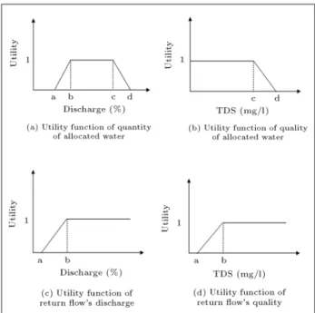
Figure 1 shows a schematic of the utility functions related to: The percentage of supplied demand (Fig-ure 1a), the quality of water allocated to each sector (Figure 1b), agricultural return ow discharge and the concentration of waste water diused into the river.
The parameters presented in Figure 1 will be determined by each sector that will be presented later. The relative weights and utility function parameters are collected by sending questionnaires to dierent stakeholders in the study area.
Figure 1. Dierent kind of utility functions for dierent kinds of conict.
OPTIMIZATION MODEL
Equation 3 shows the objective function of the op-timization model, providing the optimal quality and quantity of water allocation to each sector and optimal return ows. In the formulation, the objective function is the multiplication of each of the utility functions subtracted from their point of disagreement for every sector (agricultural, industrial, and domestic), selected withdrawal options and water storage in the reservoir for hydropower generation.
Maximize Z =Y12
m
n
a
Y
a=1
(fa;m(Aa;m) da;m)wa
!
na
Y
a=1
(fa;r;m(Ra;m) da;r;m)war
!
na
Y
a=1
(fa;c;m(Ca;m) da;c;m)wac
!
ne
Y
g=1
(fc;g;m(Cg;m) dc;g;m)wgc
!
ne
Y
g=1
(fq;g;m(Qg;m) dq;g;m)wg
!
ni
Y
i=1
(fi;m(Ri;m) di;m)wi
!
ni
Y
i=1
(fi;c;m(Ci;m) di;c;m)wic
!
ni
Y
i=1
(fi;w;m(Ci;w;m) di;w;m)wiw
!
nd
Y
d=1
(fd;m(Sd;m) dd;m)wi
!
nd
Y
d=1
(fd;c;m(Cd;m) dd;c;m)wdc
!
nd
Y
d=1
(fd;w;m(Cd;w;m) dd;w;m)wdw
!
(fs;m(Sm+1) ds;m)ws
!
: (3)
Subject to:
Rm;y = R1;m;y+ R2;m;y+ + RP;m;y Rm;min;
m = 1; ; 12; (4)
St+1= St+ It Rt Lt; t = 1; ; T; (5)
0 Ri;m;y Ri;max 8 m; y; (6)
Cm;y= g(T; w; Cin; Tin; I; Ri) 8 m; y; (7)
Cg;m;y= h(T; w; Cm;y; Rm;y) 8 m; y; (8)
where:
St: reservoir storage at the beginning of time
period t (million cubic meters), Rm;y: total release during month m in year y
(million cubic meters),
Cm;y: average concentration of water quality
variable in reservoir release during month m in year y (million cubic meters), Rm;min: in-stream ow in month m (million
cubic meters),
Ri;m;y: reservoir release from outlet i, during
month m in year y (million cubic meters), Ri;max: capacity of outlet i (million cubic meters),
Rt: total release during the time period t
(million cubic meters),
It: inow in operation time period t (million
cubic meters),
Lt: total loss during the operation time
period t due to evaporation and inltration (million cubic meters), Cin: time series of the concentration of
reservoir inow water quality (mg/l), Cg;m;y: river ow concentration in downstream of
river in month m,
g: a function that is presented by the reservoir water quality simulation model, determining the average concentration of water quality variable released from the reservoir,
h: a function that is presented by the river water quality simulation model
determining the concentration of the water quality,
T : time series of air temperature (C),
Tin: time series of inow water temperature
(C),
I: inow time series (million cubic meters), Ri: time series of release from outlet i
(million cubic meters).
Equation 7 shows the reservoir outow quality in each month as a function of the time series of
inow quality and quantity, outow from dierent gates and, also, the time series of climate conditions. This function can be implicitly obtained using a reservoir water quality simulation model. Equation 8 shows river water quality at control point g, in each month, as a function of the time series of return ow quality and quantity, quantity and quality of the outow from the upstream reservoir and, also, the time series of climatic conditions. This function can be implicitly obtained using a river water quality simulation model.
SIMULATION MODEL
Two water quality simulation models are linked with the optimization model. The rst model is used for simulation of reservoir water quality and the second one is used for river water quality simulation. The reservoir water quality simulation is used to model the outlets release quality, as well as the temporal and spatial variation of the water quality concentration in the reservoir. The basic equation of the water quality simulation model developed in this study is based on a one-dimensional advection-dispersion mass transport equation. The river water quality simulation is used to model quality variation along the river, according to agricultural return ows and industrial and domestic wastewater discharged into the river.
Reservoir Simulation
WQRRS (Water Quality for River-Reservoir Systems), a water quality simulation model, is linked with the optimization model to determine the quality of outlet release, as well as the temporal and spatial variations of the concentration of water quality variables in the reservoir. The basic equation of this water quality simulation model is based on the one-dimensional advection-dispersion mass transport equation, which is numerically integrated over space and time for each of the water quality constituents.
In the water simulation model, deep reservoirs are represented conceptually by a series of horizontal slices, each of which is characterized by a surface area, thickness and volume. The assembly of layered volume elements is a geometric representation, in discredited form, of the actual reservoir. This one-dimensional representation has been shown to ade-quately represent the water quality condition in many deep and well stratied reservoirs by Willey et al. (1996) [22]. Within each slice, the water is assumed to be fully mixed and only the vertical gradient is retained. The inter-element mass transport and the fundamental principle of the conservation of heat are represented by the following dierential equation model of the dynamics of temperature within each uid element.
V@T
@t = zQz @T
@z + zAzDz @2T
@z2 + QITI Q0T
+AchH T@V@t; (9)
where:
T : water temperature (C),
V : volume of uids element (m3),
t: time (s),
z: space coordinates (m), Qz: inter-elemet ow (m3/s),
Az: element surface area normal to the direction
of ow (m2),
Dz: eective diusion coecient (m2/s),
Qi: internal inow (m3/s),
Ti: inow water temperature (C),
Q0: lateral release (m3/s),
Ah: element surface (m2),
H: external heat sources and sinks (J/m2/s),
: water density (kg/m3),
c: specic heat of water (J/kg/C).
Vertical advection is aected by the inow and the release from the reservoir. Thus, the computation of zones of distribution and withdrawal for inows and releases is important in the development of the simulation model. Vertical advection is the net inter-element ow, which results in a continuity of ow for all elements. Eective diusion is the other transport mechanism used in the model to transport water quality constituents between elements. The eective diusion is composed of molecular and turbulent diu-sion, as well as convective mixing. This coecient is calculated using the following equations (also discussed in the HEC (1992) manual [23]):
DC= A1 if E Ecritical; (10)
DC= A2EA3 if E > Ecritical; (11)
E =1
@
@z; (12)
where:
DC: eective diusion coecient (m2/s),
A1: empirical coecient (m 1),
Ecritical: water column stability or normalized
density gradient (m 1),
A2; A3: empirical.
In order to simulate the Karkheh reservoir using the WQRRS model, the model is calibrated using metrological data in the study area and a measurement of water temperature and TDS concentration informa-tion. The results of model calibration are shown in Figure 2.
Figure 2. Result of reservoir water quality model calibration.
River Simulation
The basic equation of the water quality simulation model developed in this study is based on a one-dimensional advection-dispersion mass transport equa-tion, which is numerically integrated over space and time for each water quality constituent. This equation includes the eects of advection, dispersion, diusion, constituent reactions and interactions, and the ow sources and sinks. For any constituent concentration, c, the mass transport can be written as follows:
@M @t =
@ AxDL@x@c
@x
@ (Axuc)
@x + (Axdx) dc dt + S;(13) where:
M: the pollutant mass in the control volume (M), x: the distance along the river (L),
t: time,
c: the concentration of the pollutant (ML 3),
Ax: the cross sectional area (L2),
DL: the dispersion coecient (L2T 1),
u: the mean velocity,
S: the external source or sink (LT 1),
dx: computational element length (L).
Considering M = V c, where V is the incremental volume, (V = Axdx) and the steady state condition of
the ow in the stream, namely @Q
@t = 0, Equation 8 can
be written as follows: @c
@t =
@ AxDL@x@c
Ax@x
@ (Axuc)
Ax@x +
dc dt +
S
V: (14)
The terms on the right-hand side of the equation represent dispersion, advection, constituent changes and external sources/sinks, respectively. dc=dt refers only to the constituent changes, such as growth and
decay, and should not be confused with the term @c=dt, which is the local concentration gradient. The term @c=dt includes the eect of constituent changes, as well as dispersion, advection, source/sinks and dilutions. Changes that occur to individual constituents or par-ticles, independent of advection, dispersion and waste input, are dened by the term [24]:
dc=dt = rc + p; (15)
where r is the rst order rate constant, (T 1), and p is
the internal constituent sources and sinks, (ML 3T 1)
(e.g., nutrient loss from algal growth, benthos sources etc.).
For numerical solution of the above equations, an implicit backward nite dierence method, developed by Brown and Barnwell (1987) is used in this study [24]. In order to simulate the water quality variation along the Karkheh River according to water withdrawal and discharge by dierent users, the simulation model is calibrated for the study area. Figure 3 shows the comparison between river water quality simulation results and the concentration measurement in the study area.
SEQUENTIAL DYNAMIC GENETIC ALGORITHM
Genetic algorithms are adaptive methods trying to imitate biological and genetic processes and can suc-cessfully be applied to optimization problems. The main eld of application of GAs includes problems with high complexity and non-linear behavior, such as quality and quantity water allocation. More details of genetic algorithms can be obtained from the works of Michalewicz (1992) and Gen and Cheng (2000) [25,26]. Genetic algorithms usually consist of the following steps:
1. Encoding decision variables and placing them in a
chromosome, which is a string of encoded decision variables,
2. Creating an initial population (rst generation), 3. Determination of tness for every chromosome (set
of decision variables) in the current population (tness evaluation),
4. Setting the probability for mutation and crossover, 5. Selecting better chromosomes for mating (match-ing) and running a crossover operator for shuing the selected chromosomes,
6. Performing mutation for selected chromosomes, 7. Repeating steps 3 to 6 to obtain the optimal or near
optimal solutions.
In other words, GAs starts with a population of chromosomes and later combines them, through genetic operators, to produce better-t chromosomes. GAs do not guarantee that a new solution will be better than the previous one, however, they guarantee that the probability of being better is higher [27].
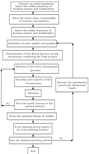
Simple genetic algorithms can be used for reser-voir operation; however, when water quality issues are included, chromosome length and computational problems are considerably increased. Considering the computational burden of the problem, in this study, a new GA-based optimization algorithm, entitled Se-quential Genetic Algorithms (SGA), proposed by Ker-achian and Karamouz [13], is used, which is based on the sequential game theory. In this methodology, the number of chromosome genes (chromosome length) is sequentially increased to eectively lead the initial feasible solutions to the global optimal solution. In this study, the gene values are the monthly release from the dierent outlets. As can be seen in Figure 4, in the rst step, a small record of quantitative and qualitative characteristics of inow is selected and the optimal monthly releases from outlets are obtained using the traditional GA-based optimization model. Then, the chromosome length is increased sequentially and the optimum solution of the rst step is located in the second part of the new chromosomes. Each step can vary from one month to 1 or 2 years. The step length is determined, based on the convergence characteristics of the GA model. This sequential method eectively reduces the computational burden of GA-based models in the long-term planning and management of water resources. Ganji et al. (2006) compared SGA with the other optimization techniques, such as GA, DP, SDP and BSDP and the performance of SGA showed an improvement compared to alterna-tive techniques [28].
Figure 4. Flowchart of the SGA model.
Encoding and Creating an Initial Population The prior requirement for coding a problem is to represent every potential solution by nding a suitable representation of the parameters of the problem and placing them in a string. The common representation method is to use binary values. An overview of other possible methods is given in [26]. The encoded parameter is referred to as a gene and a string of genes (chromosome) represents one possible solution to the problem.
In the past 10 years, various encoding methods have been proposed to provide eective GA models. In this study, a binary coding is used to represent the genes' value. In the binary encoding method, the large jumps in variable values between generations, proposed by Goldberg (1989), can be limited using gray coding [27]. In this method, which has been used in this study, the binary representation of each
variable changes in each sequence with no more than one binary digit. This binary encoding and discretiza-tion of decision variables can eectively reduce the computational burden of the problem. The details of encoding methods can be obtained in the work of Gen and Cheng (2000) [26].
Fitness Evaluation and Selection of Chromosome
The evolutionary process consists of several steps. In the rst step, the tness of each chromosome (the goodness of each solution) in the population is de-termined. In the second step (the selection phase), better chromosomes are selected for the next gener-ations. In the, so called, \mimicking the biological process" of the survival of the ttest, as stated by Burn and Yulianti (2001), the solution that has a higher level of tness, is more likely to be selected. In the next steps, selected chromosomes are shued or recombined using a crossover reproduction opera-tor [12].
In this study, the tness of each chromosome is calculated, based on the value of the Nash product, i.e., consisting of water quality and quantity allocation from the river and quantity and quality of waste loads from return ows. Some useful chromosome selection methods, such as Roulette Wheel, Tournament, Linear Ranking, Exponential Ranking and Truncation Selec-tion and their properties, were discussed by Cantu-Paz (2002) [29]. The more general methods are Tournament and Roulette Wheel selection. In the rst method, a group of individuals are chosen randomly and the individual with the highest tness is selected for inclusion in the next generation. This process is repeated until appropriate numbers of individuals are selected for the new generation. The Roulette Wheel selection is the simplest method that selects the best chromosome, according to the ratio of t-ness of each chromosome to the sum of all tt-ness values related to all chromosomes. In this paper, the Tournament selection, which is widely used in the literature, such as [12,13], is selected for the SGA-based models.
Crossover and Mutation
The reproduction operators, known as crossover and mutation, create new chromosomes. Crossover op-erators randomly select a pair of chromosomes that perform well from the mating pool and, by exchanging important building blocks between the two, a new pair is obtained. Michalewicz (1992) described three crossover methods, namely, one-point, two-point and uniform crossover, but there is no consensus among in-vestigators as to whether or not there is a generally
su-perior crossover method [25]. Crossover occurs between two selected chromosomes with a specic probability (Pc). The one point crossover, which has been selected
for this study, randomly chooses a position (gene) in the chromosome and new chromosomes are obtained by swapping all genes after that position. Mutation is an important process that can provide diversity and new genetic information to the population, while preventing premature convergence to local optimal solutions. The mutation operator changes the bit value randomly (e.g. number one becomes zero and vice-versa), with a probability of Pm.
CASE STUDY
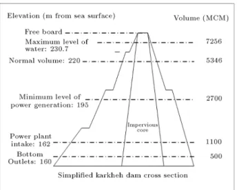
The proposed optimization/simulation procedure is used for optimal operation of the Karkheh river-reservoir system in the southern part of Iran. The Karkheh reservoir, with a volume of 7600 million cubic meters, supplies the demands of industrial, agricultural and environmental sectors. Figure 5 shows a schematic of the elevation and volume characteristics of the Karkheh dam.
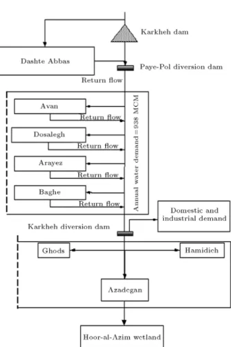
The salinity of inow to the reservoir and return ows, as well as the considerable rate of evaporation in the study area, may cause the salinity of the water in the system, so that the allocated water violates the standards in future conditions. The Karkheh dam has three outlets and one spillway, which can be used for selective withdrawal. There are six agricultural plains, an industrial complex, two towns and one termination point (Hoor-Al Azim Wetland), downstream of the Karkheh reservoir, which is presented in Figure 6. For a 50-year planning horizon, each chromosome in the SGAQ model has 12000 genes, according to the following formula and Figure 6:
Figure 5. Schematic of elevation and volume characteristics of the Karkheh dam.
Figure 6. Schematic diagram of dierent users in the study area.
[12 month50 years (9 users (quantity allocation) + 6 users (quantity return) + 2 users (quality return) + 3 outlets (quantity))]:
The utility functions of dierent decision makers of the system are considered as follows.
Environmental Sector
The environmental water quantity and quality in the Karkheh River is the main concern of this sector. The available data shows that a discharge of 80 MCM per month is needed for the Karkheh ecosystem; the environmental utility function for river ow (fq;g;m)
and water quality (fc;g;m) in control point g in month
m is formulated as follows: fq;g;m(Qg;m) =
8 > < > :
1 if Qg;m 80 MCM
1 0:033(80 Qg;m) if 50 Qg;m< 80 MCM
0 if Qg;m< 50 MCM (16)
fc;g;m(Cg;m) =
8 > > > < > > > :
0 if Cg;m 2500 mg/l
1 0:0007(Cg;m 1200) if 1200
Cg;m<2500 mg/l
1 if Cg;m 1200 mg/l
(17)
where Qg;m and Cg;m are the in-stream ow and the
concentration of the indicator water quality variable at control point g in month m.
Agricultural Sector
The main objective of this sector is to have a water supply with an acceptable quality to meet their demand with a reduction in return ow removal cost. The utility of this sector, related to the water supply, is based on water supply reliability gures. Considering the importance of the agriculture water supply in the study area, the most favorite range is 80 to 100 percent. Therefore, the utility function for a water supply to agricultural zone a(fa;m) is assumed as follows:
fa;m(Aa;m) =
8 > < > :
1 if Aa;m> 80;
1 0:017(80 Aa;m) if 20 < Aa;m 80
0 if 0 < Aa;m 20
(18) where fa;m is the utility functions related to water
supply and Aa;m is the percentage of the supplied
agricultural water demand in agricultural zone a in month m.
As treatment of agricultural return ow is not cost eective, the volume of agricultural return ow is usually reduced. The utility function for the volume of agricultural return ow in zone a in month m(fa;r;m)
is considered to be as follows: fa;r;m(Ra;m) =
8 > < > :
1 if Ra;r;m > 80
1 0:017(80 Ra;m) if 20 < Ra;r;m 80
0 if 0 < Ra;r;m 20
(19) where fa;r;mis the utility function related to return ow
discharge and Ra;r;m is the percentage of conventional
return ow from agricultural zone a in month m discharged to the river.
For agricultural water quality, the favorite range is less than 1500 mg/l in TDS concentration. Therefore, the utility function of this sector for concentration of allocated water to agricultural zone a(fa;m) is assumed
to be as follows: fa;c;m(Ca;m) =
8 > < > :
1 if Ca;m 1500
1 0:00067(Ca;m 1500) if 1500<Ca;m<3000
0 if Ca;m 3000 (20)
where fa;c;m is the utility function related to the
allocated water quality and Ca;m is the quality of the
supplied agricultural water in agricultural zone a in month m.
Industrial Sector
The main objective of this sector is to have a water supply according to industrial demand, with acceptable quality and reduction in waste water treatment cost. The utility function of the decision makers in this sector, for reliability of the industrial water supply, is as follows:
fi;m(Ri;m) =
8 > < > :
1 if Ri;m > 85
1 0:018(85 Ri;m) if 30 < Ri;m 85
0 if 0 < Ri;m 30
(21) where fi;m is the utility functions related to the
relia-bility of the water supply to industrial unit u(Ri;m).
The most preferred range for the salinity of the allocated water for industrial units is less than 1500 mg/l. Therefore, the utility function of the decision makers in this sector for allocated water concentration is assumed to be as follows:
fi;c;m(Ci;m) =
8 > < > :
1 if Ci;m 1500
1 0:00067(Ci;m) if 1500 < Ci;m 3000
0 if Ci;m> 3000
(22) where fi;c;m is the utility function related to the
allocated water quality to ith industrial unit (Ci;m).
For reducing the industrial pollution load dis-charged to the river, the concentration of industrial wastewater should be reduced. The utility function for the salinity of industrial wastewater in unit i in month m(fi;m) is considered as follows:
fi;m;w(Ci;m;w) =
8 > < > :
1 if Ci;m;w> 4000
1 0:0003(4000 Ci;m;w) if 1000<Ci;m;w<4000
0 if Ci;m;w< 1000 (23)
where fi;m;wis the utility function related to
wastewa-ter concentration and Ci;m;wis the wastewater salinity
zone i in month m discharged to the river.
Water and Wastewater Sector
The main objective of these companies is to have a water supply with acceptable quality to meet domestic demands and wastewater collection and disposal. The utility function of the decision makers in this sector, for reliability of the domestic water supply, is assumed to be as follows:
fd;m =
8 > < > :
1 if Sd;m > 94
1 0:0156(94 Sd;m) if 30 < Sd;m < 94
0 if 0 < Sd;m 30
(24) where fd;m is the utility function related to domestic
water supply reliability and Sd;m is the percentage of
the supplied domestic water demand.
As domestic allocated water, the most favorite range for the salinity of domestic water quality is less than 1200 mg/l. Therefore, the utility function of the decision makers in this sector, for allocated water salinity, is as follows:
fd;c;m(Cd;m) =
8 > < > :
1 if Cd;m 1200
1 0:0033(Cd;m 1200) if 1200 < Cd;m< 1500
0 if Cd;m 1500 (25)
where fd;c;m is the utility function related to the
allocated water salinity to dth residential region unit (Cd;m).
For reducing the domestic pollution load dis-charged into the river, the salinity of domestic waste water should be reduced. The corresponding utility function is as follows:
fd;w;m(Cd;w;m) =
8 > < > :
1 if Cd;w;m 2000
1 0:00067(2000 Cd;w;m) if 500<Cd;w;m<2000
0 if Cd;w;m 500 (26)
where fd;w;m is the utility function related to
wastew-ater salinity and Cd;w;m is the wastewater salinity
discharged from residential region d in month m. Water Supply and Energy Production Sector The main objectives of this sector are electrical power generation and water storage for future demands. The utility function of this sector, for reliability of the energy supply, is assumed as follows:
fe;m=
8 > < > :
1 if Ee;m 90
1 0:025(90 Ee;m) if 50 Ee;m< 90
0 if 0 < Ee;m 50
(27) where fe;m is the utility function related to energy
supply reliability and Ee;m is the percentage of the
supplied water demand in month m.
The reservoir storage utility is developed, con-sidering the minimum and maximum allowable water storage and water level over the hydropower intake each month. The utility function of the decision makers in this sector, for reservoir water storage, is as follows: fs;m(Sm+1) =
8 > > > > > > > > < > > > > > > > > :
0 if St+1 424 million m3
0:0013
(St+1 424) if 424 < St+1< 2250 million m3
1 if 2250
St+1< 7257 million m3
0 if St+1> 7257 million m3
(28)
where fs;m is the utility function related to reservoir
storage and Sm+1is the reservoir storage at the end of
month m.
RESULT AND DISCUSSION
In this study, the historical data of 50 years of monthly stream ow quality and quantity (1945-1995) has been used for water allocation from the Karkheh reservoir considering the quality issues. The average inow of Karkheh River at the Paye-Pole station (near the Karkheh dam) for this period is 475 MCM/month. There has been a drought period of 12 years duration in the historical inow time series. In this drought period, the mean inow discharge was about 322 MCM/month. Figure 7 shows the Karkheh reservoir volume variation during optimization periods. According to the op-timization results, it was only during the drought period that nearly 80% of the agricultural demand was supplied and the other demands were supplied completely.
The developed water quality simulation model is calibrated and veried using the available data from climatic and hydrometric stations in the region. The results show that the model can be eectively used in the proposed reservoir operation model. In Figure 8, the concentration of TDS in the inow to the Karkheh reservoir is compared with the concentration of water released from the reservoir. As shown in Figure 8, the variation of inow concentration is between 400 to 1400 mg/l and the variation of release concentration
Figure 7. Variation of reservoir volume during
optimization period (maximum and minimum volume of reservoir decrease during operation period, because of sedimentation).
Figure 8. TDS concentration of inow to the reservoir vs. TDS concentration of water release from the reservoir.
is between 600 to 1100 mg/l. The results show that the proposed model can be eectively used for opti-mizing release salinity from the reservoir by selective withdrawal.
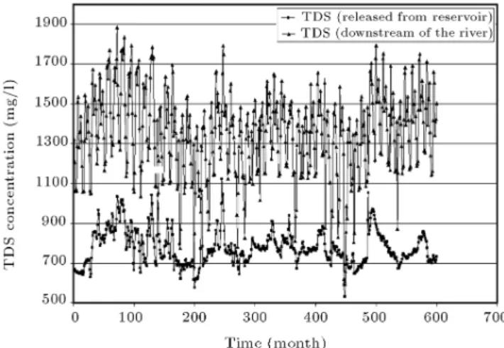
In Figure 9, the TDS concentration variation released from the reservoir and the TDS concentration variation downstream of the river (Hoor-Al-Azim) are compared. The result of the river water quality management model shows that, in 75 percent of the simulation period, the TDS concentration discharges to the Hoor-Al-Azim has only a 20 percent deviation from water quality standards. In other words, 75 percent of the time, TDS concentration is less than 1500 mg/l (12001:2 = 1440).
The results show that this model can eectively be used for river water quality management and for predicting the monthly fraction removal of point sources. In order to evaluate the performance of the optimization results, the reliability of supplying
Figure 9. The TDS concentration variation released from the reservoir vs. the TDS concentration variation
downstream of the river (Hoor-Al-Azim).
demand is calculated. The reliability of allocated water can be dened as the number of supplying demand divided by the number of time demand not satised.
Table 1 presents the reliability of optimal values of allocated water quality and quantity to dierent
water users, treatment levels of domestic and industrial wastewaters and the removal fraction of agricultural return ows to the evaporation ponds. The result of the suggested model shows that more than 80 percent of downstream water demands can be provided at the development stage. Results show that the TDS concentration downstream of the river will be reduced about 200 mg/l over the planning horizon of 50 years. The results of the optimization model are used for generating Karkheh reservoir operation policies, considering selective withdrawal from dierent outlets. The result is also used for generating river water quality management policies. In this paper, because of the complexity of quality and quantity operation rules, the Articial Neural Network (ANN) is used for generating operation and allocation rules.
In this study, dierent ANNs have been tested and a multilayer feed forward network has been selected, based on its better performance.
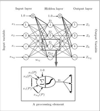
Figure 10 shows dierent components of a typical three-layered feed forward articial neural network. As can be seen in this gure, each node, j, receives incoming signals from every node, i, in the previous
Table 1. Reliability of allocated water quality and quantity to dierent parts of system. Sectors 100%
Satisfaction
90% Satisfaction
80% Satisfaction Domestic Quantity allocation 100 100 100
Quality allocation 98 100 100 Industrial Quantity allocation 100 100 100 Quality allocation 100 100 100 Abbas (Agriculture) Quantity allocation 80 85 100 Quality allocation 10 20 100 Avan Quantity allocation 65 70 100 Quality allocation 100 100 100 Dosalegh Quantity allocation 65 70 100 Quality allocation 100 100 100 Arayez Quantity allocation 65 70 100 Quality allocation 100 100 100 Bagheh Quantity allocation 65 70 100 Quality allocation 100 100 100 Karkhe Soa Quantity allocation 59 65 99
Quality allocation 100 100 100 Environment Quantity allocation 100 100 100 Quality allocation 26 43 70
Figure 10. Typical three-layer feed forward articial neural network.
layer. Associated with each incoming signal, (xi), to
node j, a weight, (wji), is assigned. The eective
incoming signal, (sj), to node j is the weighted sum
of all the incoming signals as follows: sj=
n0
X
i=0
wjixi; (29)
where x0 and wj0 are called the bias and the bias
weight, respectively. The output of node j is yj. More
detailed information about the training of the ANNs can be found in Hsu et al. (1995) [30].
Two kinds of policies/operating rules are gen-erated for the Karkheh reservoir operation and river water quality, as discussed in the following sections. Karkheh Reservoir Operation Policy
This policy is for the total quality and quantity of the Karkheh release in each month, with respect to inow and TDS concentration, reservoir volume in the previous month and water quality stratication in the Karkheh reservoir. The number of layers in the ANN network is 3, the considered transition function for layer 1 and layer 2 is tansig and for the third layer is pureline. The number of neurons in each layer is 4, 9 and 7, respectively. The number of iterations is set as 5000. The root mean square error for the calibration and validation of the ANN model are 0.12 and 0.15278, respectively.
The reservoir operation rule suggested by the ANN simulation and the framework of the suggested
model follows that as described in Equation 30. Fig-ure 11 shows, the result of the ANN model validation for monthly water release from the Karkheh reservoir. Table 2 shows the error analysis of the ANN model simulation results for the monthly water release from the Karkheh reservoir. In Figure 12, the result of the ANN model validation for the release from outlet 1 is drawn. The error analysis of this ANN model simulation is presented in Table 3.
Y = pureline(w1 tansig(w2
tansig(w3[X] + b3) + b2) + b1);
(30) where:
W1: coecient matrix for the rst layer,
W2: coecient matrix for the second layer,
W3: coecient matrix for the third layer,
b1; b2; b3: bios constants for each layer,
X: vector of independent variables consists of inow discharge to the reservoir, TDS concentration in inow, reservoir volume in the previous month, water demand in each month and stratication of water quality at each gate; this vector has 21 elements,
Y : vector of dependent variables, consists of reservoir release discharge and quality, the release from each outlet; this vector has 7 elements.
Table 2. Error analysis of ANN model simulation results for monthly water release from the Karkheh reservoir.
Error Range 10% 20% 30% 50% Percent of
Simulated Data in Each Error Range
34 58 80.5 94
Figure 11. ANN model validation for monthly water release from the Karkheh reservoir.
Figure 12. ANN model validation for monthly water release from outlet 1 of the Karkheh reservoir.
Table 3. Error analysis of ANN model simulation results for monthly water release from outlet 1 of the Karkheh reservoir.
Error Range 10% 20% 30% 50% Percent of
Simulated Data in Each Error Range
29 49.5 63.5 81.5
Karkheh River Water Quality Management Policy
This policy is for river water quality management that contains the allocated water for stakeholders, the quantity of return ow from agricultural demands and the quality of industrial and urban wastewater, with respect to the discharge and TDS concentration of the river upstream of each point source. The framework of this network is the same as the previous network, with the exception of the number of neurons in the rst layer, which is 2, and the third layer, which is 17. The root mean square errors for calibration and validation of the ANN model are 0.1 and 0.1434, respectively. The same expression as Equation 30 is used for generating a river water quality management policy. The following independent and dependent variables are dened as follows:
X: Vector of independent variables, consists of dis-charge and TDS concentration of the river up-stream of each point source with two elements, Y : Vector of dependent variables consists of allocated
water to stakeholders, the quantity of return ow from agricultural demands and the quality of in-dustrial and urban waste water with 17 elements. In Figure 13, a result of validation for allocated water to the Abbas agriculture region is drawn as an example. In Table 4, simulated and forecasted data with dierent errors are presented.
Figure 13. ANN model validation for monthly allocated water to the Abbas agriculture region.
Table 4. Error analysis of ANN model simulation results for monthly water allocated to the Dasht-e-Abbas agriculture unit.
Error Range 10% 20% 30% 50% Percent of
Simulated Data in Each Error Range
74 93.5 100 100
SUMMARY AND CONCLUSION
In this study, the Nash theory is used for resolving the conict between dierent users. A Sequential Genetic Algorithm model (SGA), which is also referred to as dynamic GA, is developed to solve the large scale conict resolution model with 12000 alternatives. In the SGA model, the relative weights of the util-ity functions, related to water qualutil-ity, water supply, wastewater treatment, pollution load removal fraction and reservoir storage volume, are considered.
The proposed model can signicantly improve the reliability in qualitative and quantitative aspects of water allocation. In this model, selective withdrawal for optimizing river water quality downstream of the reservoir and river water quality management is also considered.
The model has been applied to the Karkheh river-reservoir system in Iran and the results of the optimiza-tion model are used for generating operating rules for water allocation and water quality management in the study area.
ACKNOWLEDGMENTS
This study was partially supported by a research con-tract with the Water Resources Management Organi-zation of the Ministry of Energy, entitled \Qualitative and Quantitative Planning and Management of Water Resources with Emphasis on Conict Resolution".
A part of this paper will be presented at the 7th international conference in Civil Engineering (ICCE7) at Tarbiat Modarres University, Tehran, I.R. Iran. REFERENCES
1. Wolf, A.T. \Conict and corporation along interna-tional waterways", Water Policy, 1(2), pp 251-265 (1998).
2. Wolf, A.T., Conict Prevention and Resolution in Water Systems, Edward Elgar Publishing Ltd., Chel-tenham, UK (2002).
3. Kaplan, E. \Reservoir optimization for water quality control", PhD. Dissertation, University of Pennsylva-nia, Philadelphia, USA (1974).
4. Fontane, D., Labadie, J. and Loftis B. \Optimal control of reservoir discharge quality through selective withdrawal", Water Resources Research, 17(6), pp 1594-1604 (1981).
5. Nandalal, K.D.W. and Bogardi, J.J. \Reservoir man-agement for improving river water quality", Proc. of Water Resources Management Under Drought or Water Storage Conditions, Rotterdam, pp 257-264, Holland (1995).
6. Hayes, D.F., Labadie, J.W., Sanders, T.G. and Brown, J.K. \Enhancing water quality in hydropower system operations", Water Resources Research, 34(3), pp 471-480 (1998).
7. Palmer, R.N., Werick, W.J., Mac Ewan, A. and Woods, A.W. \Modeling water resources opportuni-ties, challenges and trade-os: The use of shared vision modeling for negotiation and conict resolution", Proc. 26th Annual Conf., Water Resour. Plann. Manage., ASCE, Tempe, AZ, USA (June 1999).
8. Palmer, R.N., Ryu, J., Jeong, S. and Kim, Y.O. \An application of water conict resolution in the Kum river basin, Korea", Proceeding of ASCE Envi-ronmental and Water Resources Institute Conference, Virginia, May 19-22 (2002).
9. Coppla, E., Szidarovszky, F., Poulton, M., Spayd, S. and Roman, E. \Balancing risk with water supply for a public well eld", J. Water Res. Plann. Manage. Div. Am. Soc. Civ. Eng., 126(2), pp 1-36 (2001).
10. Karamouz, M., Szidarovszky, F. and Zahraie, B., Water Resources Systems Analysis, Lewis Publishers, USA (2003).
11. Sasikumar, K. and Mujumdar, P.P. \Fuzzy optimiza-tion model for water quality management of a river system", Journal of Water Resources Planning and Management, ASCE, 124(2), pp 79-88 (1998). 12. Burn, D.H. and Yulianti, S. \Waste-load allocation
using genetic algorithms", Journal of Water Resources Planning and Management, ASCE, 127(2), pp 121-129 (2001).
13. Kerachian, R. and Karamouz, M. \Waste-load allo-cation model for seasonal river water quality man-agement: Application of sequential dynamic genetic
algorithms", Journal of Scientia Iranica, 12(2), pp 117-130 (2005).
14. Karamouz, M. and Kerachian, R. \Optimal operation of reservoir systems considering the water quality: Ap-plication of stochastic sequential genetic algorithms", Proceedings of ASCE World Water and Environmental Resources Congress 2004, Salt Lake City, Utah (2004). 15. Le-Huu, T. \Potential water conicts and sustainable management of international water resources systems", Water Resources Journal of United Nations Economic and Social Commission for Asia and the Pacic (UN-ESCAP), No.ST/ESCAP/SER.C/210, pp 1-13 (2001). 16. Varian, H.R., Intermediate Microeconomics: A Mod-ern Approach, W.W. Norton & Company Inc., p 662 (1995).
17. Thomson, W. \Cooperative models of bargaining", Handbook of Game Theory with Economic Applica-tions, Aumann, R.J. and Hart, S., Eds., II, Elsevier, Amsterdam, pp 1237-1284 (1994).
18. Richards, A. and Singh, N. \Two level negotiations in bargaining over water", Proceedings of the Interna-tional Game Theory Conference, Bangalore, India, pp 1-23 (1996).
19. Shahidehpour, M., Yamin, H. and Li, Z., Market Operations in Electric Power Systems, John Wiley and Sons, New York, pp 191-232 (2001).
20. De Marchi, B., Funtowicz, S.O., Cascio, S.L. and Munda, G. \Combining participative and institutional approaches with multicriteria evaluation. An empirical study for water issues in Troina, Sicily", Ecological Economics, 34(2), pp 267-282 (2000).
21. Ganji, A., Kamgar, A.K., Khalili, D. and Sepaskhah, A.R. \The application of conict resolution funda-mentals in irrigation scheduling under uncertain situ-ations", Proceeding of Water Resources Management Conference, Wessex Institute of Technology, Gran Canaria (2002).
22. Willey, R.G., Smith, D.J. and Duke, J.H. \Modeling water resources systems for water quality manage-ment", Journal of Water Resources Planning and Management, ASCE, 122(3), pp 171-179 (1996). 23. Hydrologic Engineering Center (HEC), HEC-5Q
Sim-ulation on Flood Control and Conservation Systems, Appendix on Water Quality Analysis, Davis, Calif (1992).
24. Brown, L.C. and Barnwell, O., The Enhanced Stream Water Quality Models, QULA2E and QUAL2E-UNCAS: Documentation and User Manual, EPA (1987).
25. Michalewicz, Z., Genetic Algorithms + Data Struc-tures = Evolutionary Programs, Springer, New York, USA (1992).
26. Gen, M.R. and Chang, L., Genetic Algorithm and Engineering Optimization, Wiley Europe Publication (2000).
27. Goldberg, D.E., Genetic Algorithms in Search, Op-timization and Machine Learning, Addison-Wesley, Reading, Mass, USA (1989).
28. Ganji, A., Karamouz, M. and Khalili, D. \Devel-opment of stochastic conict resolution models for reservoir operation, the value of players information availability and cooperative behavior", Advances in Water Resources Research (2006).
29. Cantu-Paz, E. \Order statistics and selection methods of evolutionary algorithms", Info. Proc. Letters, 82, pp 15-22 (2002).
30. Hsu, K., Gupta, H.V. and Sorooshian, S. \Articial neural network modeling of the rainfall-runo pro-cess", Water Resources Research, 31(10), pp 2517-2530 (1995).