Sharif University of Technology
Scientia IranicaTransactions E: Industrial Engineering www.scientiairanica.com
Computing centroid of general type-2 fuzzy set using
constrained switching algorithm
A. Doostparast Torshizi
a, M.H. Fazel Zarandi
a,c;and I. Burhan Turksen
b,c a. Department of Industrial Engineering, Amirkabir University of Technology, Tehran, P.O. Box 15875-5513, Iran. b. Department of Industrial Engineering, TOBB Economics and Technology University, Sogutozu, Ankara, Turkey. c. Knowledge/Intelligence Systems Laboratory, Department of Mechanical & Industrial Engineering, University of Toronto,Toronto, Canada.
Received 17 February 2014; received in revised form 21 August 2014; accepted 8 December 2014
KEYWORDS General type-2 fuzzy sets;
Constrained Switching (CS) algorithm; Type-reduction; -plane representation; Enhanced Karnik-Mendel (KM) algorithms.
Abstract.Centroid of general type-2 fuzzy set can be used as a measure of uncertainty in highly uncertain environments. Computing centroid of general type-2 fuzzy set has received an increasing research attention during recent years. Although computation complexity of such sets is higher than that of interval type-2 fuzzy sets, with the advent of new representation techniques, e.g. -planes and z-Slices, computation eorts needed to deal with general type-2 fuzzy sets have decremented. A very rst method to calculate the centroid of a general type2 fuzzy set was to use KarnikMendel algorithm on each -plane, independently. Because of the iterative nature of this method, running time in this approach is rather high. To tackle such a drawback, several emerging algorithms such as Sampling method, Flow algorithm, and, recently, Monotone Centroid-Flow algorithm have been proposed. The aim of this paper is to present a new method to calculate centroid intervals of each -plane, independently, while reducing convergence time compared with other algorithms like iterative use of Karnik-Mendel algorithm on each -plane. The proposed approach is based on estimating an initial switch point for each -plane. Exhaustive computations demonstrate that the proposed method is considerably faster than independent implementation of existing iterative methods on each -plane. © 2015 Sharif University of Technology. All rights reserved.
1. Introduction
General Type-2 Fuzzy Sets (GT2 FSs) are Type-2 (T2) fuzzy sets with a secondary membership function which can take on any value between zero and one. This concept was rst introduced by Zadeh [1]. GT2 FSs have more degrees of freedom so that they are capable of dealing with high level uncertainties in a more intuitive manner than Interval Type-2 (IT2) fuzzy sets and traditional type-1 fuzzy sets. As a result, GT2 FSs have received much attention during last years and they have been successfully applied to many real
*. Corresponding author. Tel.: +98 21 6454 5378
E-mail address: [email protected] (M.H. Fazel Zarandi)
engineering and medical cases [2,3]. Some of the most successful engineering and medical applications of the T2 fuzzy systems are data classication [4,5], expert systems and function approximation [6-9], and medical treatments [10,11]. Nearly, most of these applications were based upon IT2 FSs since computational complex-ity of GT2 FSs was high. Meanwhile, with the advent of new representation methods, GT2 FSs are going to be widely applied in various scientic areas.
As a crucial uncertainty representation measure, computing the centroid of GT2 FS is mandatory when performing type-reduction in Fuzzy Logic Systems (FLSs) [12,13]. This issue has been an active eld of research during recent years, but there are serious problems in this way since there is not a closed-form
solution to nd the centroid of a GT2 FS, directly. To date, several type-reduction methods have been proposed to deal with IT2 FSs of which a new geometric method representing eective inference techniques to deal with T2 fuzzy sets has been presented in [14]. Recently, Kumbasar et al. [15] have presented the exact inversion of decomposable interval type-2 fuzzy logic systems. Then, based on the decomposition property of IT2 FLSs, the analytical formulation of the inverse of an IT2 FLS is driven for the interval switching point of Karnik-Mendel (KM) type-reduction algorithm.
Computing the exact value of centroid of a GT2 FS is only possible through considering the entire embedded sets of the GT2 FS. Such a thing is nearly impossible since the number of embedded sets are too large to be considered in a limited time. Hence, other methods, such as sampling [16], have been proposed to facilitate the process of type-reduction of GT2 FSs. In [16], the authors present a sampling method to nd the centroid of GT2 FSs, which is close to the exact optimal centroid of that GT2 FS.
To date, several other practical methods have been presented to nd the centroid of a GT2 FS. Coup-land [17] uses x-coordinate of the geometric centroid of the 3-D membership function of fuzzy sets. The main disadvantage of this method lies in the fact that the GT2 FS is directly converted to a crisp value so that a huge amount of uncertainty is lost and the resultant centroid does not provide an appropriate measure of uncertainty. In another research, Lucas et al. [18] present an ad hoc method to compute the centroid of GT2 FSs using the entire vertical slices. Note that each vertical slice is a T1 FS in itself. Ignoring other geometric properties of GT2 FSs, this method results in a centroid whose domain is exactly the same as the domain of the primary variable of the considered FS. Therefore, this method can be a reliable measure of uncertainty.
One of the most prominent representation methods of GT2 FSs is to decompose them into several -planes. The concept of -planes has been thoroughly discussed by Mendel et al. [19]. Such a representation oers a computationally ecient framework to deal with GT2 FSs. To facilitate the process of type-reduction, Liu [20] has utilized the concept of -planes to nd the centroid of a GT2 FS. He decomposes each GT2 FS into several planes which are IT2 FSs. Then Karnik-Mendel (KM) algorithm is applied to nd the centroid of each -plane. Finally, the entire obtained centroids are aggregated and the centroid of the GT2 FS is obtained. This method is appropriate in theoretical studies, but it is not much useful when applied to real world problems since it is rather time consuming. Based on weaknesses of Liu's work, Yeh et al. [21] present an enhanced algorithm in order to speed up the process of type-reduction. Their main
concentration is nding the initial switch point for each -plane in order to enhance eciency of the type-reduction process. Recently, Wu et al. [22] also proposed a new fast type-reduction method based on improvements performed on the Liu's [20] approach. In [23], Greeneld et al. conducted a study on comparing Liu's -plane decomposition method with direct approach of sampling presented in [16]. In another study, Greeneld and Chiclana [24] investi-gate which of the type-reduction methods working on IT2 FSs are better to be coupled with the Liu's -plane decomposition method. These methods are the KM algorithm, the collapsing method [25], and the Nie's approach [26]. A comprehensive description is represented in [27], which tries to discuss the basic concepts of GT2 FSs. Also in [28], defuzzication of GT2 FSs based on discretization process has been experimentally evaluated.
Recently, based on mathematical properties of -planes, two ecient algorithms have been developed for computing the centroid of GT2 FSs. The main dierence of these methods lies in the fact that despite previous type-reduction methods, which implement Enhanced KM (EKM) or KM algorithms on each -plane, they do not need to perform iterative time consuming procedures for each plane. The rst algo-rithm is called Centroid Flow (CF) algoalgo-rithm [29]. CF algorithm starts from an initial point in the rst -plane and nds its centroid bounds. This starting point is the same centroid interval of the lowest -plane which is obtained using KM or EKM iterative algorithms. Then, using derivatives of the secondary membership functions in each -plane for the entire discretized primary variables, centroid intervals of each -plane ow to its upper plane while having some changes. It is proved that the CF algorithm is 75%-80% faster than the KM algorithm and 50%-75% faster than the EKM method [30]. Then, Zhai and Mendel enhanced the CF algorithm and presented a more powerful approach based on the CF algorithm [30,31]. The CF algorithm suers from some drawbacks. The main drawback of this algorithm is that due to the interrelations of this algorithms, computational errors of this algorithm gradually accumulate as the algorithms goes to other -planes. This will denitely aect the accuracy of the nal T1 type-reduced FS. Also, it does not yield similar results obtained from independent application of KM/EKM algorithms on each -plane.
Recently, based on the CF algorithm, Linda and Manic [30] have proposed an enhanced version of the CF algorithm called Monotone CF (MCF) algorithm. In the MCF algorithm, monotonicity of secondary membership functions has been used towards develop-ing a fast algorithm for type-reduction purposes. MCF has several features including: a) It leads to identical centroids as KM/EKM algorithms; b) It is easy to
implement; and c) It is faster than its counterpart, i.e. the CF algorithm. Despite CF algorithm which begins from the lowest plane and needs to have an initial start-ing point calculated by KM/EKM algorithms, MCF eliminates the need for using KM/EKM algorithms and also can be initiated from any deliberate -plane. One of the main advantages of the MCF algorithm is that it is rather easy to implement and it does not need to compute the derivatives of the secondary membership functions on each -plane.
Both CF and MCF algorithms start to work from an initial point and both are faster than the existing procedures, like KM and EKM; but in both methods, it is necessary to nd the upper and lower membership values for each -plane. On the other hand, CF algorithm does not yield solutions identical to the obtained solutions from KM/EKM algorithms. In this way, two fundamental questions arise: 1) How can we compute centroid endpoints of each independent -plane identical to the results of KM/EKM algorithms, but in a much faster manner? 2) To speed up the process, how can we develop a new way to nd the centroid of each -plane without the need to compute centroids of the upper or the lower planes as occurs in CF and MCF algorithms? According to these questions, it can be observed that the capability of computing centroid of each plane without any need to nd the centroids of the preceding planes is achieved in KM/EKM algorithms, but they are slower than CF and MCF algorithms. To boost them up, funda-mental changes are needed to be implemented in the EKM/KM algorithms so that their starting switching points in each -plane be close to the optimal switch points of that -plane as much as possible. Since the proposed method in this paper concentrates on the initial switch points of each -plane, it will be called \Constrained Switching (CS) algorithm". This method will be discussed in the incoming sections of the paper. Based on the above discussions, the main contri-bution of this paper can be listed as follows:
Presenting novel methods for nding good initial switching points for type-reduction of IT2 FSs to reduce the number of iterations needed to reach the optimal switching points;
Providing some lemma and theorems on charac-teristics of -planes and their inuences on type-reduction of GT2 FSs;
Presenting two fast iterative algorithms based on the concept of -planes for the type-reduction of GT2 FSs.
The rest of the paper is organized as follows. In Section 2, the basic concepts of GT FSs will be re-viewed. Dierent type-reduction methods for GT2 FSs are discussed in Section 3 and the proposed approaches are discussed in Section 4. In Section 5, comparative experiments are represented and conclusion remarks will be given in Section 6.
2. General type-2 fuzzy sets
In this section, we briey review the basic concepts of GT2 FSs and -plane representation procedure of GT2 FSs.
2.1. General type-2 fuzzy sets
According to [32], a GT2 FS ~A is expressed on a universe of discourse X using its corresponding T2 membership function A~(x; u), where x 2 X and u 2
Jx:
~ A =
Z
x2X
Z
u2Jx
A~(x; u)=(x; u); Jx [0; 1]; (1)
where x is the primary variable value, u denotes the secondary variable, Jx denotes an interval between
the lower and the upper membership functions, and A~(x; u) denotes the secondary membership function.
Note thatRR represents union over the entire possible values of x; u and A~(x; u). A schematic view of a GT2
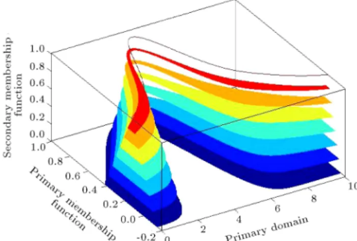
FS with Gaussian secondary is depicted in Figure 1(a).
Figure 1. a) Schematic view of a GT2 FS ~A with mixed Gaussian secondary MF. b) -plane representation of the GT2 FS ~A.
According to John and Mendel [33], there are two important representations for GT2 FSs: the Vertical Slice representation and the Wavy Slice representation. A GT2 FS ~A can be represented by its vertical slices. Vertical slice of ~A can be obtained by consid-ering a specic point in universe of discourse, such as x = x0. Then, the vertical slice
~
A(x0; u) of the fuzzy
membership function A~(x; u) can be obtained. In
fact, vertical slices at each point represent a secondary membership function, A~(x = x0; u), for x0 2 X and
8u 2 Jx0 [0; 1]:
A~(x = x0; u)
Z
u2Jx0
fx0(u)=u; Jx0 [0; 1]; (2)
where fx0(u) is amplitude of the secondary membership
function and fx0(u) [0; 1]. Suppose that the entire
domain has been discretized into N samples. Then, the GT2 FS ~A can be represented as an aggregation of its entire vertical slices as follows [30]:
~ A =XN
i=1
"Z
u2Jxi
fxi(u)=u
#
=xi: (3)
The other well-known representation method for a GT2 FS ~A has been provided as follows [30]:
~ A = [
8 ~Ae
~
Ae: (4)
Here, ~A has been represented by the union of all its embedded T2 FSs. An embedded T1 fuzzy set of ~A,
~
Ae is described by an MF uA~e : X ! [0; 1], where
uA~e2 Jx. ~Ae is expressed as [29]:
~ Ae=
Z
x2Xu=x; u 2 Jx; (5)
where the embedded T1 FS ~Ae, which corresponds
to an embedded T2 FS ~Ae, contains the primary
memberships of that ~Ae.
2.2. -Plane representation of general type-2 fuzzy sets
The concept of -planes has also been developed by several other researchers, independently, i.e. Tahayori et al. [34], Chen and Kawase [35], and Liu [20]. The notations on the concept of -plane are adopted from [19].
An -plane of a GT2 FS ~A is the union of the entire primary memberships of ~A whose secondary grades are greater than or equal to (0 1). -plane of ~A is denoted by ~A.
~ A=
Z
8x2X
Z
8u2Jx
f(u; x)jfx(u) g : (6)
An -cut of the secondary MF A~(x) is represented by
sA~(xj):
SA~(xj) = [SL(xj); SR(xj)] : (7)
As a result, ~Acan be constructed as a composition of
all -cuts of all of its secondary membership functions, i.e.:
~ A=
Z
8x2XSA~(xj)=x
= Z
8x2X
Z
8u2[SL(xj);SR(xj)]
u !
=x: (8)
Using -planes, we can redene the well-known deni-tion of Footprint Of Uncertainty (FOU). FOU is equal to the lowest -plane, i.e.:
FOU( ~A) = ~A0: (9)
According to Zhai and Mendel [29], each -plane is bounded from above by its upper membership function, A~(xj), and from below by its lower membership
func-tion, A~(xj) . The upper and the lower membership functions of a plane ~A can be described in terms of
-cuts as follows: A~(xj) =
Z
8x2XSR(xj); (10)
A~(xj) = Z
8x2XSL(xj): (11)
A schematic view of -planes for the GT2 FS ~A is depicted in Figure 1(b). Each -plane is indeed an interval T2 FS with the centroid CA~ (x), e.g. centroid
of ~A on the -plane `'. Liu [20] states that the centroid of a GT2 FS ~A, CA~(x), is a composition of its all
-planes, i.e.: CA~(x) =
[
2[0;1]
=CA~ (x): (12)
Note that centroid of each -plane, CA~ (x), has a lower
and an upper bound so that the centroid of a GT2 FS ~
A can be rewritten as Eq. (13): CA~(x) =
[
2[0;1]
=hcl( ~A=); cr( ~Aj)
i
: (13)
For a better understanding, a 3D view of a GT2 FS with Gaussian primary membership function and triangular secondary membership function represented by its -planes is illustrated in Figure 2. In this gure, there are eight -planes, each in a dierent color. These -planes are IT2 FSs. For more intuitive gures, the reader can refer to [29,30].
Figure 2. A GT2 FS represented by its -planes. 3. Type-reduction of general type-2 fuzzy sets Here, we will have a brief review on the KM type-reduction algorithm. Although KM is basically devel-oped for ITS FSs, it can be iteratively used for type-reduction purposes implemented on each -plane of a GT2 FS.
3.1. Karnik-Mendel (KM) algorithm
KM algorithm starts with nding an initial mean average, and then iteratively continues until converging to the left and right endpoints of the centroid intervals. The KM algorithm to compute Cl( ~A) is given in
Algorithm 1.
The algorithm to nd the Cr( ~A) is quite similar
to the above algorithm, so we leave it behind. In Algorithm 1, L and N represent the left switch point and the total number of primary domain members, respectively.
3.2. Enhanced KM algorithm (EKM)
In order to expedite the computation process of nd-ing the centroid endpoints of an IT2 FS, Wu and Mendel [36] proposed an enhanced version of the KM (EKM) algorithm which nds an initial switching point for the IT2 FS in such a way that the number of iter-ations for convergence decreases remarkably. However, EKM is basically designed to deal with IT2 FSs, and in order to nd the centroid of a GT2 FS, it should be iteratively applied to dierent -planes of the GT2 FS. Therefore, it is still time consuming to use EKM in GT2 FSs. Some new works on type-reduction algorithms can be found in [37,38].
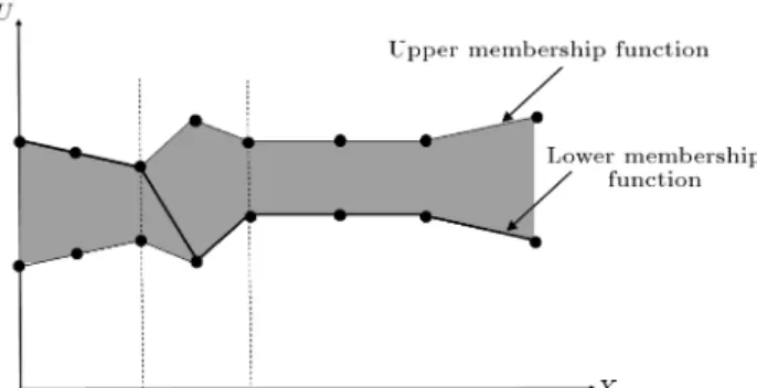
Switch points are members of the primary do-main. These points are used as a switch between the lower and the upper membership functions of any IT2 FS. Switch points were rst introduced by Karnik and Mendel to nd the left and right endpoints of the corresponding type-reduced T1 FSs of IT2 FSs. During the iterative procedure of computing the left and right centroid endpoints, an initial centroid is obtained using the traditional COG defuzzication method. Then, using this initial centroid, left and right switch points are computed until the nal left and right centroid endpoints are reached. A schematic view of left and right switch points are demonstrated in Figure 3.
In Figure 3, the upper and the lower membership functions of an IT2 FS accompanied by the primary domain values are represented. As can be observed, the right dashed line denotes the initial switch point and the left dashed line denotes the nal left switch point where a shift from the upper membership function to the lower membership function occurs in order to
Figure 3. A schematic view of the left switch point in an IT2 FS.
Figure 4. A schematic view of the right switch point in an IT2 FS.
compute the left centroid endpoint of the IT2 FS. The same story is true in Figure 4.
Based on the above discussions, we present a fast iterative procedure, especially designed for GT2 FSs. The proposed method is able to estimate an initial value for both left and right switch points in each -plane such that the initial switch points are close to the switch points of the left and right centroid endpoints in each -plane and the algorithm converges to these endpoints faster than the KM/EKM algorithms. The proposed algorithm tries to nd a good initial switch point, but the procedure of converging to the left and right centroid endpoints of each -plane is similar to that of KM/EKM methods.
4. Constrained switching algorithm
Switch points are one of the main tools in nding the centroid endpoints of IT2 FSs. Moreover, there is not a closed form solution to nd centroid of an IT2 FS. In order to compute centroid endpoints of an IT2 FS, some algorithms, such as EKM/KM, use an initial switch point and then check other remaining switch points in order to gain the termination criterion of the algorithm. Our experiments show that the initial switch point is crucial in decreasing the number of iterations to gain the left or right endpoints of each centroid interval [39,40]. KM and EKM algorithms use a constant procedure to nd a starting switch point for
computing centroid intervals of each -plane. Our aim is to nd a good initial switch point in order to expedite the process of converging to the centroid endpoints of each -plane. A comprehensive comparison between various type-reduction algorithms is presented in [41]. For more information about the applications of T2 FSs, please refer to [61-64].
In this section, several lemma and theorems are provided, and then the CS algorithm will be presented. 4.1. Theorems
Secondary membership functions of a GT2 FS ~A can have dierent shapes such as triangular, trapezoidal, Gaussian, and etc. When secondary membership functions have a single apex, such as Gaussian or triangular, ~A becomes a T1 FS and its centroid will be a single point. On the other hand, when secondary membership functions are trapezoidal, ~A becomes an IT2 FS so that its centroid will be an interval. Also, according to the monotonicity property for the GT2 FSs ~A, if 1 2, then [30]:
cl( ~Aj1) cl( ~Aj2); cr( ~Aj1) cr( ~Aj2): (18)
Suppose that the apex of the secondary membership grade of the GT2 FSs ~A in the point x is calculated as follows:
Apex(x) = Sl(xj1) + w (Sr(xj1) Sl(xj1)) ;
0 w 1; (19)
where Sl(xj1) is the left primary membership value at
the -plane ~A1 for the primary domain value of x,
Sr(xj1) is the right primary membership value at the
-plane ~A1 for the primary domain value of x, and w
is a weighting coecient.
Suppose that the secondary membership func-tions are triangular or Gaussian. Also w can take any value from interval [0, 1]. When w increases from 0 to 1, Apex(x) approaches Sr(xj1). Since Eq. (19) holds
for the entire discrete values of the primary domain, by increasing w from 0 to 1, Apex(x) gets close to A~(xj0). On the other hand, when w decrements to 0,
Apex(x) gets close to A(xj0)~ . Moreover, for any value of w, centroid of ~A is xed. Suppose ~cl( ~Aj) to be
an approximation for the left centroid endpoint of the GT2 FS ~A at the -plane `'. This approximated left centroid endpoint is obtained based on the connection line between the left centroid endpoints of the -planes
~
A0 and ~A1 as follows:
~cl( ~Aj) = (cl( ~Aj1) cl( ~Aj0)) + cl( ~Aj0); (20)
where ~cl( ~Aj) denotes an approximation of cl ( ~Aj),
cl( ~Aj1) represents left centroid endpoint of the GT2
FS ~A at the highest -plane, and cl( ~Aj0) represents
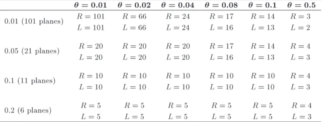
Table 1. The number of left and right switching points for dierent numbers of planes and discretization levels of the primary domain.
= 0:01 = 0:02 = 0:04 = 0:08 = 0:1 = 0:5 0.01 (101 planes) R = 101
L = 101
R = 66 L = 66
R = 24 L = 24
R = 17 L = 16
R = 14 L = 13
R = 3 L = 2 0.05 (21 planes) R = 20
L = 20
R = 20 L = 20
R = 20 L = 20
R = 17 L = 16
R = 14 L = 13
R = 4 L = 3 0.1 (11 planes) R = 10
L = 10
R = 10 L = 10
R = 10 L = 10
R = 10 L = 10
R = 10 L = 10
R = 4 L = 3 0.2 (6 planes) R = 5
L = 5
R = 5 L = 5
R = 5 L = 5
R = 5 L = 5
R = 5 L = 5
R = 4 L = 3 -plane. Now, we can dene an initial switching point
for the left endpoints of centroid intervals.
Proposition 1. Consider ~L as the largest value from the primary domain to be less than or equal to ~cl( ~Aj)
in Eq. (20). Then, ~L can be used as an initial switching point in the iterative procedure to nd the left centroid endpoint of the GT2 FS ~A at the level .
Proof of this proposition is represented in Ap-pendix A.
In a similar way, suppose that KM/EKM algo-rithms have been applied to ~A1 and ~A0. Then, the
connection line between cr( ~Aj0) and cr( ~Aj1) will be as
follows: ~cr( ~Aj) =
cr( ~Aj1) cr( ~Aj0)
+ cr( ~Aj0); (14)
where ~cr( ~Aj) is an approximation for cr( ~Aj), cr( ~Aj1)
represents the right centroid endpoint of the GT2 FS ~
A when = 1, and cr( ~Aj0) denotes the right centroid
endpoint of the GT2 FS ~A when = 0.
Proposition 2. Consider ~R; as the smallest value from the primary domain, to be larger than or equal to ~cr( ~Aj) (21). Then, ~R can be used as an initial
switching point in the iterative procedure to nd the right centroid of the GT2 FS ~A at the level `'. Proof of this proposition is similar to the proof of Proposition 1. It will be shown in the next section that the pro-posed initial switch points at any -level are very good estimations to be replaced in the iterative procedures such as KM/EKM algorithms.
Theorem 1. When the apex of the secondary mem-bership function is bowed to the UMF or LMF of the lowest -plane, the connection line between cl( ~Aj1) and
cl( ~Aj0) and also the connection line between cr( ~Aj1)
and cr( ~Aj0) can be an estimation for the left and
right endpoints of the centroid interval of each -plane, respectively. Proof of Theorem 1 is represented in Appendix B.
Theorem 2. Suppose Ts to be the distance between
two consecutive -planes and to be the distance be-tween two consecutive values in the discretized primary domain. Then, for any value of , the right and the left switch points of each centroid interval at each -level will be unique if Ts .
Proof. To prove this theorem, several exhaustive experiments have been conducted and precision of the theorem has been proved, experimentally. These ex-periments are performed on the dataset ~F represented in Eqs. (22) and (23).
According to the performed computations repre-sented in Table 1, as it can be viewed, if the discretiza-tion distance is small, then the number of -planes will not have signicant impacts on switching points and each pair of values of CR and CL will have its unique
switching point at each -plane. Now, for each -plane, if the discretization distance of the primary domain is large, then switching points for CRand CLin several
-planes may be identical. According to these exhaustive computations, it can be concluded that the values of CRand CLin each -plane may have unique switching
points when Ts where is the distance between two
consecutive points on the discretized primary domain and Ts is the distance between two consecutive
-planes. In Table 1, the secondary membership function is considered to be triangular, where L is the number of left switching points and R is the number of right switching points.
Graphical representations of these experiments are represented in Figures 5-8. From these gures it can apparently be concluded that each -plane may have unique switching points when Ts . This claim
can be observed in Figures 5-7 apparently. 4.2. Constrained switching algorithm
According to Proposition 1, Proposition 2, Theorem 1, and Theorem 2, the steps of the CS algorithms are presented for computing both left and right centroid endpoints for each -level.
Figure 5. Distribution on the right and left endpoints of centroid intervals when Ts= 0:01.
Figure 6. Distribution on the right and left endpoints of centroid intervals when Ts= 0:05.
Figure 7. Distribution on the right and left endpoints of centroid intervals when Ts= 0:1.
Figure 8. Distribution on the right and left endpoints of centroid intervals when Ts= 0:2.
Steps of the CS algorithm for computing the left centroid endpoints of the GT2 FS ~A at each -level are shown in Algorithm 2.
Also, steps of the CS algorithm for computing the right centroid endpoints at each -level are represented in Algorithm 3.
In the original KM algorithm, the initial switching point for the entire -planes is obtained through an ordinary average of the upper and the lower mem-bership values for the entire primary domain. Ac-cording to Theorem 1, when the apex of the sec-ondary membership function is bowed to the LMF, the left centroid endpoints in each plane tend to become less than their corresponding values of ~cl( ~Aj)
in Eq. (20). In the same manner, right centroid endpoints tend to become more than ~cl( ~Aj). Since
the KM algorithm is originally designed for IT2 FSs, it does not take into account slopes of secondary membership functions. But our presented algorithms use these slopes so that their initial switching points are very close to the optimal switch points for each -plane. In contrast to the independent application of KM/EKM algorithm for each -plane, this property leads to a decrease in the number of iterations for each -plane to reach the left and right centroid endpoints.
Indeed, the CS algorithm tries to modify the orig-inal KM/EKM algorithms through a good estimation of the initial switch points at each -plane. This will denitely reduce the number of iterations at each -plane, but it does not change the general methodology of reaching the nal left and right endpoints of centroid intervals of the -plane. Hence, the CS algorithms have a reasonable computational complexity while reach-ing the same exact centroid endpoints as KM/EKM methods. This claim will be analyzed in the next section.
4.3. Computational complexity
The CS algorithms try to reduce the number of iter-ations in the original KM/EKM algorithms at each -plane through estimating an initial switching point based on a guess made by the connection line between the highest and the lowest -planes. The CS algorithm for both left and right centroid endpoints is iterated k times, where k represents the total number of -planes. According to Theorem 2, which determines the appropriate number of discretized values of the primary domain, suppose that the primary domain is represented by N discrete values. At each iteration, for each -plane, since an initial estimation is obtained for the starting switch point, the maximum iterations for each -plane will be N
2. On the other hand, since
this process is performed twice for each -plane, the maximum iterations will be N. If KM algorithm is applied independently to each -plane, we have to
Algorithm 2. The CS algorithm for computing the left centroid endpoints of the GT2 FS ~A.
Algorithm 3. The CS algorithm for computing the right centroid endpoints of the GT2 FS ~A. call Eq. (14) twice, which is of order 2N. In the CS
algorithm, this has been eliminated, and after just one iteration, the initial left and right switch points are obtained. Therefore, for each -plane, the total count will be N + 2. Hence, the entire count for the CS algorithm will be k(N + 2), which is of order O(Nk).
In comparison with the CF (and ECF [60]) al-gorithm, which is of order O (Nk + max(N; k)), the proposed algorithm has a smaller computational com-plexity while having the capability of reaching the values of the left and right endpoints of centroid intervals at each -plane.
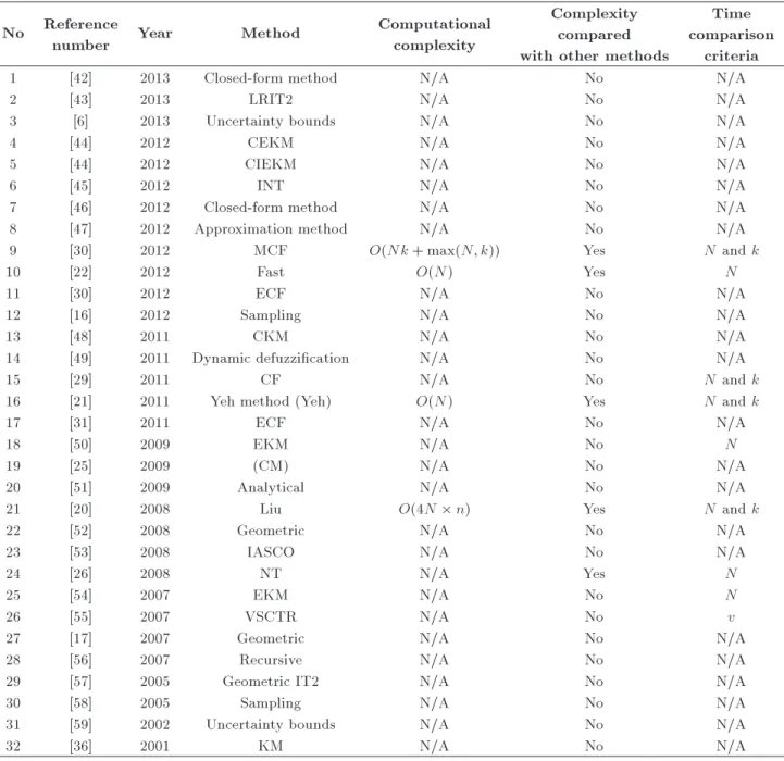
In Table 2, a brief review on computational complexities of the existing approaches is presented. It is apparent that the CS algorithms represent a lower computational complexity compared with other state-of-the-art approaches.
5. Comparative studies
This section provides an exhaustive numerical analysis on the proposed approaches compared to the other existing methods. To implement the proposed algo-rithms, two benchmark GT2 FSs, which are widely used in the literature, are adopted. The rst GT2 FS
~
F is composed of two Gaussian membership functions. The upper and the lower membership functions are represented in Eqs. (22) and (23):
UMFF OU( ~F )(x) = max
exp
(x 3)2
8
; 0:8 exp
(x 6)2
8
; (22)
LMFF OU( ~F )(x) = max
0:5exp
(x 3)2
2
Table 2. Complexity analysis. No Reference
number Year Method
Computational complexity
Complexity compared with other methods
Time comparison
criteria
1 [42] 2013 Closed-form method N/A No N/A
2 [43] 2013 LRIT2 N/A No N/A
3 [6] 2013 Uncertainty bounds N/A No N/A
4 [44] 2012 CEKM N/A No N/A
5 [44] 2012 CIEKM N/A No N/A
6 [45] 2012 INT N/A No N/A
7 [46] 2012 Closed-form method N/A No N/A
8 [47] 2012 Approximation method N/A No N/A
9 [30] 2012 MCF O(Nk + max(N; k)) Yes N and k
10 [22] 2012 Fast O(N) Yes N
11 [30] 2012 ECF N/A No N/A
12 [16] 2012 Sampling N/A No N/A
13 [48] 2011 CKM N/A No N/A
14 [49] 2011 Dynamic defuzzication N/A No N/A
15 [29] 2011 CF N/A No N and k
16 [21] 2011 Yeh method (Yeh) O(N) Yes N and k
17 [31] 2011 ECF N/A No N/A
18 [50] 2009 EKM N/A No N
19 [25] 2009 (CM) N/A No N/A
20 [51] 2009 Analytical N/A No N/A
21 [20] 2008 Liu O(4N n) Yes N and k
22 [52] 2008 Geometric N/A No N/A
23 [53] 2008 IASCO N/A No N/A
24 [26] 2008 NT N/A Yes N
25 [54] 2007 EKM N/A No N
26 [55] 2007 VSCTR N/A No v
27 [17] 2007 Geometric N/A No N/A
28 [56] 2007 Recursive N/A No N/A
29 [57] 2005 Geometric IT2 N/A No N/A
30 [58] 2005 Sampling N/A No N/A
31 [59] 2002 Uncertainty bounds N/A No N/A
32 [36] 2001 KM N/A No N/A
Performance measure:
T: Time; C: Computational complexity; N: Sample size; n: An integer less than 10; k: Number of -planes; and v: Number of vertical slice.
0:4 exp
(x 6)2
2
: (23)
The second GT2 FS ~G has a piecewise linear FOU with the following upper and lower membership functions:
UMFF OU( ~G)(x) = max 8 < : 2
4(7 x)=4; 3 < x 7(x 1); 1 x 3 0; otherwise 3 5 ; 2
4(16 2x)=5; 6 < x 8(x 2)=5; 2 x 6 0; otherwise 3 5
9 =
;; (24)
LMFF OU( ~G)(x) = max 8 < : 2
4(7 x)=6; 4 < x 7(x 1); 1 x 4 0; otherwise 3 5 ; 2
4(x 3)=6; 3 x 5(8 x)=9; 5 < x 8 0; otherwise 3 5
9 =
; : (25)
The simulations are performed on an Acer 4750 running Windows 7 Ultimate and MATLAB 2011a with Intel
.
Core i5 CPU at 2.4 GHz and 4 GB RAM.chosen to be trapezoidal and triangular. The tops for the left and right points of the triangular membership functions are calculated by Eq. (19) and the left and right points of the trapezoidal membership functions are calculated by Eqs. (26) and (27). It should be noted that in Eqs. (19), (26), and (27), we have used these values for the weighting coecient, w = 0; 0:25; 0:5; 0:75; 1.
Apexleft(x) = LMFF OU( ~A0)(x) + 0:6w
UMFF OU( ~A0)(x) LMFF OU( ~A0)(x)
; (26) Apexright(x) = LMFF OU( ~A0)(x) 0:6(1 w)
UMFF OU( ~A0)(x) LMFF OU( ~A0)(x)
: (27) 5.1. An illustrative example for Theorem 1 To illustrate Theorem 1, the left and right centroid endpoints of ~A0 and ~A1 of the GT2 FS ~F are
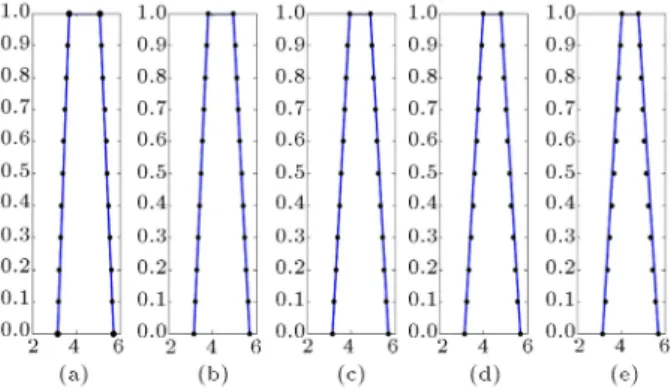
com-puted when the secondary membership functions are triangular and trapezoidal. Then, the connection lines between left centroid endpoints of these two -planes and also the connection line between their right centroids are drawn. Finally, considering Ts = 0:1,
the centroid endpoints of each -plane are computed directly using the EKM algorithm. It can be observed that in Figures 9 and 10, the centroid endpoints are distributed in the vicinity of the connection lines when w changes. Connection lines in both Figures 9 and 10 are drawn in blue for dierent values of w. When w increases, the left and right centroid endpoints of each -plane tend to get into the inner side of connection line. But for lower values of w, centroid endpoints of planes get into the outer side of the connection lines. This implies that the connection lines can be a good initial estimation for computing the centroid endpoints of each -plane and their intersection with each value of can play the role of a good initial switching point.
Figure 9. Centroids of the GT2 FS ~F with triangular secondary membership functions: a) w = 0; b) w = 0:25; c) w = 0:5; d) w = 0:75; and e) w = 1.
Figure 10. Centroids of the GT2 FS ~F with trapezoidal secondary membership functions: a) w = 0; b) w = 0:25; c) w = 0:5; d) w = 0:75; and e) w = 1.
5.2. Accuracy tests
It is important to see whether the proposed approaches have ne performance in contrast to the existing approaches or not. The CS algorithm is iterative, so its results can be compared with two other well-known iterative methods, e.g. KM/EKM algorithms. We have computed centroids of the two GT2 FSs ~F and ~G with two dierent kinds of secondary mem-bership functions: triangular and trapezoidal. In order to form the apex of the secondary membership functions, ve dierent values for have been consid-ered. Since KM and EKM algorithms have identical computational results, the EKM results are reported in order to make comparisons. Computed centroids for both GT2 FSs are represented in Figures 11 and 12.
In Figures 11 and 12, EKM is used to nd the centroid intervals of six -planes with Ts = 0:2.
These centroid endpoints are shown by dots. The primary domains for both EKM and CS algorithms are discretized into 50 and 80 points for the GT2 FSs ~F and ~G, respectively. The distance between
Figure 11. Centroids of the GT2 FS ~F : (a)-(e) With trapezoidal secondary membership functions; and (f)-(j) with triangular secondary membership functions. (a), (f): w = 0; (b), (g): w = 0:25; (c), (h): w = 0:5; (d), (i): w = 0:75; and (e), (j): w = 1.
Figure 12. Centroids of the GT2 FS ~G: (a)-(e) With trapezoidal secondary membership functions; and (f)-(j) with triangular secondary membership functions. (a), (f): w = 0; (b), (g): w = 0:25; (c), (h): w = 0:5; (d), (i): w = 0:75; and (e), (j): w = 1.
the -planes for the CS algorithm is considered to be Ts= 0:1. Centroids computed by the CS algorithm are
represented with bold lines in Figures 11 and 12. As can be observed, the CS algorithm has achieved exactly the results of EKM and it can be reliably applied for type-reduction purposes of GT2 FSs. Now, the main advantages of the proposed CS algorithm in terms of running time and switching issues are discussed in comparison to with EKM/KM algorithms, which are the running time and switching issues.
5.3. Switching analysis
As noted before, the main advantage of the CS algo-rithm, compared to its rivals, lies in the fact that in the CS algorithm, initial switching points for each
-plane are obtained in such a way that the number of iterations to reach the nal switching points is much less than applying the KM/EKM algorithm in each -plane, independently.
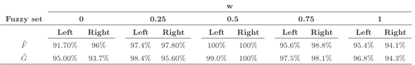
To investigate this important characteristic of the CS algorithm, another experiment is also conducted. Here, we have obtained the initial switch points and nal switch points for both left and right endpoints of centroid intervals using KM, EKM, and CS algorithms when w = 0; 0:25; 0:5; 0:75; 1. It is assumed that the distance between two consecutive -planes is 0.1. Then, for each value of w, the dierence between initial and nal switch points for each -plane is computed and their averages are recorded. These values are represented in Figure 13.
It can be observed that the capability of CS algorithm in contrast to KM and EKM methods is apparent. Even for some values of w, like 0.5 or 0.6, the average dierence between initial and nal switching points is zero. This means that for the entire -planes, the CS algorithm has just one iteration, while it is far from the average numbers of iterations of the KM/EKM algorithms.
The dierence between the results of CS and KM/EKM algorithms is apparent that we can even conclude that there is no need to apply KM/EKM algorithms, independently, for each -plane. In such a situation, one can compute both the left and the right centroid endpoints with the least number of iterations in a timely manner using the CS algorithm.
In Tables 3 and 4, it is shown in percent that how much the CS algorithm has decreased the average number of switching iterations compared with KM and EKM algorithms. It can be observed that the CS algorithm reduces the average number of iterations
Table 3. Reductions in the average number of switching iterations for the CS algorithm against the KM method. w
Fuzzy set 0 0.25 0.5 0.75 1
Left Right Left Right Left Right Left Right Left Right
~
F 84.10% 90% 95.2% 94.30% 100% 100% 91.9% 96.8% 91.4% 83.4%
~
G 84.20% 88.3% 94.9% 90.50% 96.8% 100% 92.4% 94.1% 88.5% 71.1%
Table 4. Reductions in the average number of switching iterations for the CS algorithm against the EKM method. w
Fuzzy set 0 0.25 0.5 0.75 1
Left Right Left Right Left Right Left Right Left Right
~
F 91.70% 96% 97.4% 97.80% 100% 100% 95.6% 98.8% 95.4% 94.1%
~
G 95.00% 93.7% 98.4% 95.60% 99.0% 100% 97.5% 98.1% 96.8% 94.3%
between 71.10% up to 100%. This is a very appropriate advantage of the CS method compared with KM/EKM algorithms.
5.4. Computational time testing
In this experiment, we have divided the secondary membership domain into 50 parts, which means that the Ts can take on 50 dierent values from this set:
f0:02; 0:04; :::; 0:98; 1g. Then for each of these 50 values of Ts, 1000 simulations are performed and the average
of computational times is recorded for each Ts value.
The computational results are reported in Figure 14. By increasing the number of discretized values of the primary domain, simulation times increase, but these increases are much less for the CS method in contrast to EKM/KM algorithms.
According to Figure 14, compared to independent use of KM algorithm for each -plane, the CS algorithm performs better. According to the literature, EKM algorithm is designed to reduce the number of iterations in order to reach the left and right endpoints of
the centroid intervals in each alpha plane. It has been proved that EKM performs faster than the KM algorithm. This has been veried in Figure 14. As can be observed, the CS algorithm performs better than the KM and EKM algorithms when applied independently.
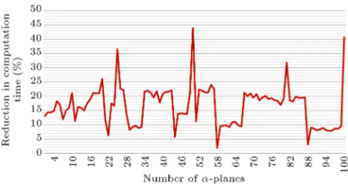
According to the simulations, the CS algorithm decreased the computational time of the KM algorithm by the average of 45% to 59%. It also improved the computational time of the EKM method up to 40%. This is an impressive result for an iterative method that makes it capable of competing with other newly developed fast methods. For a better understanding of the percentage of time reduction, in Figures 15-18, the reduction in computational time of the CS algorithm compared with the KM and EKM algorithms, on both datasets, are represented.
For a better understanding of the quality of the CS algorithms, we have provided some other exper-iments on Nie-Tan (NT), IASC, and EKMANI [62]. Results of this experiment are represented in Figure 19.
Figure 15. Reduction of computational time of the EKM algorithm when applying the CS algorithm to the dataset
~ F .
Figure 16. Reduction of computational time of the KM algorithm when applying the CS algorithm to the dataset
~ F .
Figure 17. Reduction of computational time of the EKM algorithm when applying the CS algorithm to the dataset
~ G.
Figure 18. Reduction of computational time of the KM algorithm when applying the CS algorithm to the dataset
~ G.
Figure 19. Computation times after 1000 simulations for IASC, EKMANI, NT, and CS algorithms.
Superiority of the CS algorithm over the men-tioned methods, represented in Figure 19, can be apparently observed. Here CS performs the best and IASK, EKMANI, and NT algorithms stand after the CS algorithm, respectively. This experiment veries fast performance of the CS algorithm versus some of the highly desirable approaches in the literature. 6. Conclusions
This paper addresses the type-reduction issue of GT2 FSs. The proposed algorithms are iterative and speci-cally designed for GT2 FSs. The CS algorithm operates on -planes of GT2 FSs and can nd the centroid interval of each -plane by beginning from a near optimal switching point. Basically, the main advantage of the proposed CS algorithm, compared to other
existing algorithms, can be summarized as follows: 1) The CS algorithm converges faster to the left and right centroid endpoints of each -plane, while independent application of EKM/KM algorithms on each -plane is more time consuming; 2) despite some new algorithms, such as CF and MCF, which cannot compute the centroid interval of each -plane independently, the CS algorithm can compute centroids without any need to have the centroid endpoints of the previous -plane in order to compute centroid interval of the current -plane.
We showed that the CS algorithm outperforms KM-based type-reduction algorithms and some of the state-of-the-art methods, such as EKMANI, NT, and IASC. But, still this method is iterative and there is a long way to reduce the number of iterations, and as a result, the total computation time. According to [2], z-Slices are equivalent to IT2 FSs. Therefore, they can be applied to each -plane, and as a result, the proposed method in this paper can be used when representing the GT2 FSs with z-Slices.
It should be noted that the CS algorithm is basically designed to deal with Gaussian, triangular, and trapezoidal secondary membership functions and does not handle piecewise linear or non-convex sec-ondary membership functions. Considering non-convex secondary membership functions will be the subject of our future research. Since KM-based algorithms are originally designed for IT2 FSs and as IT2 FSs are convex, it seems that -planes can no longer fulll the needs for decomposing GT2 FSs. Hence, other methods, such as direct algorithms with closed-form solutions, may be desirable.
Conict of interests. The authors declare no con-ict of interests.
References
1. Zadeh, L.A. \The concept of a linguistic variable and its approximate reasoning-II", Inf. Sci., 8, pp. 301-357 (1975).
2. Wagner, C. and Hagras, H. \Toward general type-2 fuzzy logic systems based on zslices", IEEE Trans. Fuzzy Syst., 18(4), pp. 637-660 (2010).
3. Zhai, D. and Mendel, J.M. \Uncertainty measures for general type-2 fuzzy sets", Inf. Sci., 181, pp. 503-518 (2011).
4. Lucas, L.A., Centeno, T.M. and Delgado, M.R. \Land cover classication based on general type-2 fuzzy clas-siers", Int. J. Fuzzy Syst., 10(3), pp. 207-216 (2008).
5. Zeng, J. and Liu, Z.Q. \Type-2 fuzzy Markov ran-dom elds and their application to handwritten Chi-nese character recognition", IEEE Trans. Fuzzy Syst., 16(3), pp. 747-760 (2008).
6. Fazel Zarandi, M.H., Doostparast Torshizi, A., Turk-sen, I.B. and Rezaee, B. \A new indirect approach to the type-2 fuzzy systems modeling and design", Inf. Sci., 232, pp. 346-365 (2013).
7. Aliev, R.A., Pedrycz, W., Guirimov, B.G., Aliev, R.R., Ilhan, U., Babagil, M. and Mammadli, S. \Type-2 fuzzy neural networks with fuzzy clustering and dierential evolution optimization", Inf. Sci., 181, pp. 1591-1608 (2011).
8. Melin, P., Mendoza, O. and Castillo, O. \Face recog-nition with an improved interval type-2 fuzzy logic, Sugeno integral, and modular neural networks", IEEE Trans. Syst., Man, Cyber., 41(5), pp. 1001-1012 (2011).
9. Fazel Zarandi, M.H., Faraji, M.R. and Karbasian, M. \Interval type-2 fuzzy expert system for prediction of carbon monoxide concentration in mega-cities", Appl. Soft. Comp., 12, pp. 291-301 (2012).
10. Lee, C.S., Wang, M.H. and Hagras, H. \A type-2 fuzzy ontology and its application to personal diabetic-diet recommendation", IEEE Trans. Fuzzy Syst., 18(2), pp. 374-395 (2010).
11. Di Lascio, L., Gisol, A. and Nappi, A. \Medi-cal dierential diagnosis through type-2 fuzzy sets", Proceedings of the IEEE International Conference on Fuzzy Systems, pp. 371-376 (2005).
12. Mendel, J.M., John, R.I. and Liu, F. \Interval type-2 fuzzy logic systems made simple", IEEE Trans. Fuzzy Syst., 14(6), pp. 808-821 (2006).
13. Mendel, J.M. \Type-2 fuzzy sets and systems", IEEE Comp. Int. Mag., 2(1), pp. 20-29 (2007).
14. Coupland, S. and John, R. \New geometric inference techniques for type-2 fuzzy sets", Int. J. App. Reason., 49, pp. 198-211 (2009).
15. Kumbasar, T., Eksin, I., Guzelkaya, M. and Yesil, E. \Exact inversion of decomposable interval type-2 fuzzy logic systems", Int. J. App. Reason., 54(2), pp. 253-272 (2013).
16. Greeneld, S., Chiclana, F., John, R.I. and Coupland, S. \The sampling method of defuzzication for type-2 fuzzy sets: Experimental evaluation", Inf. Sci., 189, pp. 77-92 (2012).
17. Coupland, S. \Type-2 fuzzy sets: Geometric defuzzi-cation and type-reduction", Proceedings of IEEE International Symposium on Foundations of Computa-tional Intelligence, Honolulu, USA, pp. 622-629 (2007).
18. Lucas, L.A., Centeno, T.M. and Delgado, R.M. \Gen-eral type-2 inference systems: Analysis, design, and computational aspects", Proceedings of the IEEE In-ternational Conference on Fuzzy Systems, London, UK, pp. 1107-1112 (2007).
19. Mendel, J.M., Liu, F. and Zhai, D. \-plane represen-tation for type-2 fuzzy sets: Theory and applications", IEEE Trans. Fuzzy Syst., 17 (5), pp. 1189-1207 (2009).
20. Liu, F. \An ecient centroid type-reduction strategy-for general type-2 fuzzy logic system", Inf. Sci., 178, pp. 2224-2236 (2008).
21. Yeh, C.Y., Jeng, W.H.R. and Lee, S.J. \An enhanced type-reduction algorithm for type-2 fuzzy sets", IEEE Trans. Fuzzy Syst., 19(2), pp. 227-240 (2011).
22. Wu, H.J., Su, Y.L. and Lee, S.J. \A fast method for computing the centroid of a type-2 fuzzy set", IEEE Trans. Syst., Man, and Cyber., 42(3), pp. 764-777 (2012).
23. Greeneld, S., Chiclana, F., Coupland, S. and John, R.I. \Type-2 defuzzication: Two contrasting ap-proaches", Proceedings of IEEE International Confer-ence on Fuzzy Systems, FUZZ-IEEE, Barcelona, Spain (2010).
24. Greeneld, S. and Chiclana, F. \Combining the a-plane representation with an interval defuzzication method", Proceedings of EUSFLAT-LFA, Aix-Les-Bains, France (2011).
25. Greeneld, S., Chiclana, F., Coupland, S. and John, R.I. \The collapsing method of defuzziction for dis-cretized interval type-2 fuzzy sets", Inf. Sci., 179(13), pp. 2055-2069 (2009).
26. Nie, M. and Tan, W.W. \Towards an ecient type-reduction method for interval type-2 fuzzy logic sys-tems", Proceedings of IEEE International Conference on Fuzzy Systems, FUZZ-IEEE, Hong Kong (2008).
27. Greeneld, S. and John, R.I. \The Uncertainty Asso-ciated with a type-2 fuzzy set", Chapter in Views on Fuzzy Sets and Systems from Dierent Perspectives, edited Rudolf Seising in Studies in Fuzziness and Soft Computing, series editor Janusz Kacprzyk, Springer Verlag, pp. 471-483 (2009).
28. Greeneld, S. and Chiclana, F. \Defuzzication of the discretized generalized type-2 fuzzy set: Experimental evaluation", Inf. Sci., 244, pp. 1-25 (2013).
29. Zhai, D. and Mendel, J.M. \Computing the centroid of a general type-2 fuzzy set by means of the centroid-ow algorithm", IEEE Trans. Fuzzy Syst., 19(3), pp. 401-422 (2011).
30. Linda, O. and Manic, M. \Monotone centroid ow algorithm for type-reduction of general type-2 fuzzy sets", IEEE Trans. Fuzzy Syst., 20(5), pp. 805-819 (2012).
31. Zhai, D. and Mendel, J.M. \Enhanced centroid-ow algorithm for general type-2 fuzzy sets", Proceedings of the North American Fuzzy Information Processing Society, NAFIPS, Texas, USA (2011).
32. Mendel, J.M., Uncertain Rule-Based Fuzzy Logic Sys-tems: Introduction and New Directions, Upper Saddle River, NJ: Prentice-Hall (2001).
33. Mendel, J.M. and John, R.I. \Type-2 fuzzy sets made simple", IEEE Trans. Fuzzy Syst., 10(2), pp. 117-127 (2002).
34. Tahayori, H., Tettamanzi, A.G.B. and Antoni, G.D.\Approximated type-2 fuzzy set operations", Pro-ceedings of the IEEE International Conference on Fuzzy Systems, Vancouver, Canada, pp. 1910-1917 (2006).
35. Chen, Q. and Kawase, S. \On fuzzy-valued fuzzy reasoning", Fuzzy Set. Syst., 113, pp. 237-251 (2000).
36. Karnik, N.N. and Mendel, J.M. \Centroid of a type-2 fuzzy set", Inf. Sci., 132, pp. 195-220 (2001).
37. Greeneld, S. and Chiclana, F. \Accuracy and com-plexity evaluation of defuzzication strategies for the discretised interval type-2 fuzzy set", Int. J. App. Reason., 54(8), pp. 1013-1033 (2013).
38. Chiclana, F. and Zhou, S.M. \Type-reduction of gen-eral type-2 fuzzy sets: The type-1 OWA approach", Int. J. Intell. Syst., 28(5), pp. 505-522 (2013).
39. Doostparast Torshizi, A., Fazel Zarandi, M.H. and Zakeri, H. \On type-reduction of type-2 fuzzy sets: A review", Appl. Soft Comp., 27, pp. 614-627 (2015).
40. Doostparast Torshizi, A. and Fazel Zarandi, M.H. \Hi-erarchical collapsing method for direct defuzzication of general type-2 fuzzy sets", Inf. Sci., 277, pp. 842-861 (2014).
41. Wu, D. and Nie, M. \Comparison and practical im-plementation of type-reduction algorithms for type-2 fuzzy sets and systems", IEEE Int. Conf. on Fuzzy Syst. (FUZZ-IEEE 11), Taiwan, pp. 2131-2138 (2011).
42. Ulu, C., Guzelkaya, M. and Eksin, I. \A closed form type-reduction method for piecewise linear interval type-2 fuzzy sets", Int. J. App. Reas., 54, pp. 1421-1433 (2013).
43. Chen, C.L., Chen, S.C. and Kuo, Y.H. \Reduction of interval type-2 LR fuzzy sets", IEEE Trans. on Fuzzy Syst., 22(4), pp. 840-858 (2014).
44. Liu, X., Qin, Y. and Wu, L. \Fast and direct Karnik-Mendel algorithm computation for the centroid of an interval type-2 fuzzy set", IEEE Int. Conf. on Fuzzy Syst. (FUZZ-IEEE 2012), Brisbane, Australia, pp. 1-8 (2012).
45. Mendel, J.M. and Liu, X. \New closed-form solutions for Karnik-Mendel algorithm+defuzzication of an interval type-2 fuzzy set", IEEE Int. Conf. on Fuzzy Syst. (FUZZ-IEEE 2012), Brisbane, Australia, pp. 1-8 (2012).
46. Ulu, C., Guzelkaya, M. and Eksin, I. \A new type-reduction method for piecewise linear interval type 2 fuzzy sets", 2nd World Conference on Soft Computing, W Con SC'12, Baku, Azerbaijan, pp. 494-498 (2012).
47. Garcia, J.C.F. \An approximation method for type-reduction of an interval type-2 fuzzy set based on alpha-cuts", Federated Conference on Computer Sci-ence and Information Systems, pp. 49-54 (2012).
48. Liu, X. and Mendel, J.M. \Connect Karnik-Mendel algorithms to root-nding for computing the centroidof an interval type-2 fuzzy set", IEEE Trans. on Fuzzy Syst., 19(4), pp. 652-665 (2011).
49. Ulu, M. Guzelkaya, and Eksin, T. \A dynamic de-fuzzication method for interval type-2 fuzzy logic con-trollers", IEEE Int. Conf. on Mechatronics, Istanbul, Turkey, pp. 318-323 (2011).
50. Wu, D. and Mendel, J.M. \Enhanced Karnik-Mendel algorithms", IEEE Trans. Fuzzy Syst., 17(4), pp. 923-934 (2009).
51. Greeneld, S., Chiclana, F. and Jonh, F. \Type-reduction of the discretized interval type-2 fuzzy set", IEEE Int. Conf. on Fuzzy Syst., FUZZ-IEEE, Korea, pp. 738-743 (2009).
52. Coupland, S. and John, R. \A fast geometric method for defuzzication of type-2 fuzzy sets", IEEE Trans. on Fuzzy Syst., 16(4), pp. 929-941 (2008).
53. Duran, K., Bernal, H. and Melgarejo, M. \Improved iterative algorithm for computing the generalized cen-troid of an interval type-2 fuzzy set", NAFIPS'08, New York, pp. 1-5 (2008).
54. Wu, D. and Mendel, J.M. \Enhanced karnik-mendel algorithms for interval type-2 fuzzy sets and systems", NAFIPS'07, San Diego, USA, pp. 184-179 (2007).
55. Alberto, L., Mezzadri Centeno, T. and Regattieri Delgado, M. \General type-2 fuzzy inference systems: Analysis, design and computational aspects", IEEE Int. Conf. on Fuzzy Syst. (FUZZ-IEEE 07), London, pp. 1743-1747 (2007).
56. Melgarejo, M. \A fast recursive method to compute the generalized centroid of an interval type-2 fuzzy set", NAFIPS'07, San Diego, CA, USA, pp. 190-194 (2007).
57. Coupland, S. and John, R. \Geometric interval type-2 fuzzy systems", Proceedings of EUSFLAT - LFA, pp. 449-454 (2005).
58. Greeneld, S., John, R. and Coupland, S. \A novel sampling method for type-2 defuzzication", UK Workshop Computational Intelligence, London, U.K., pp. 120-127 (2005).
59. Wu, H. and Mendel, J.M. \Uncertainty bounds and their use in the design of interval type-2 fuzzy logic systems", IEEE Trans. on Fuzzy Syst., 10(5), pp. 622-639 (2002).
60. Zhai, D. and Mendel, J.M. \Enhanced centroid-ow algorithm for computing the centroid of general type-2 fuzzy sets", IEEE Trans. Fuzzy Syst., 20(5), pp. 939-956 (2012).
61. Hagras, H. \A hierarchical type-2 fuzzy logic controller for autonomous mobile robots", IEEE Trans. Fuzzy Syst., 12(4), pp. 524-539 (2004).
62. Linda, O. and Manic, M. \Interval type-2 fuzzy voter design for fault tolerant systems", Inf. Sci., 181(14), pp. 2933-2950 (2011).
63. Lynch, C. and Hagras, C. \Using uncertainty bounds in the design of en embedded real-time type-2 neuro-fuzzy speed controller for marine diesel engines", Proceedings of the IEEE International Conference on Fuzzy Systems, Vancouver, Canada, pp. 1446-1453 (2006).
64. Wu, D. and Nie, M. \Comparison and practical im-plementation of type-reduction algorithms for type-2 fuzzy sets and systems", Proceedings of IEEE Inter-national Conference on Fuzzy Systems, FUZZ-IEEE, Taiwan (2011).
Appendix A
Proof of Proposition 1. According to monotonicity property of the secondary membership functions, this membership function can be represented as follows:
fx(u) =
8 > > > > > < > > > > > :
gx(u); u 2 (SL(xj0); SL(xj1))
hx(u); u 2 (SR(xj1); SR(xj0))
1; u 2 [SL(xj1); SL(xj1)]
0; otherwise
(A.1)
where gx(u) (hx(u)) is the function of the left (right)
side of the secondary membership function. SL(xj0)
and SR(xj0) are the lower and upper membership
values of x at the lowest -plane, respectively. Also, SL(xj1) and SR(xj1) are the lower and upper
member-ship values of x at the highest -plane, respectively. According to Eq. (19), suppose w = 0 and the secondary membership function is triangular. We have considered w = 0 since only in such a situation, the left endpoint of the centroid interval of two consecutive -planes will be in the closest condition. Then, for each -plane, such as ~A and its next -plane ~A+T, we
have:
8xSL(xj + Ts) = SL(xj); (A.2)
and:
8xSR(xjjTs) = SR(xj) +h0Ts
x(u); (A.3)
where h0
x(u) is the derivative of the secondary
member-ship (h(u)) value of x at the -level, `' represents the distance between two consecutive -planes, SL(xj)
and SR(xj) represent the left and right membership
values of x at the -plane ``, respectively. Since h0
x(u) < 0, the secondary membership
val-ues for each discretized primary domain value between two subsequent -planes decreases by Ts
h0
x(u). On the
other hand, since the secondary membership functions are triangular, the slope for any -plane is constant:
8 SR(xj) SR(xj + Ts) Cons tan t: (A.4)
According to the KM algorithm, the left endpoint of the centroid interval for the -plane ~A is computed
as follows. Note that each discretized value `i' of the primary domain is represented by xi.
CL=
PL
i= xiSR(xij) +
PN
i=L+1xiSl(xij)
PL
i=1SR(xij)j +
PN
i=L+1SL(xij)
: (A.5) According to the literature [29]:
CL+Ts=
LP+Ts
i=1 xiSR(xij + Ts) + N P i=L+Ts+1
xiSL(xij + Ts) LP+Ts
i=1 SR(xij + Ts) + N P i=L+Ts+1
SL(xij + Ts)
: (A.8)
Box I
And also for the entire values of the primary domain: SR(xj) > SR(xj + Ts): (A.7)
Then, the left endpoint of the centroid interval for the -plane ~A+Tscan be obtained by Eq. (A.8) as shown
in Box I.
Substituting Eqs. (A.2) and (A.3) in Eq. (A.8) results in Eq. (A.9) as shown in Box II. Then, based on Eq. (A.6), the non-equality (A.10), as shown in Box III, is true. According to Eq. (A.2), if the switch points in both -planes are the same, then Eq. (A.10) should be transformed to an equality. Therefore, suppose that the switch points in both -planes ~A and ~A+Ts
are identical. In such a situation, the proportion of numerator to denominator in both fractions of Eq. (A.10) should be the same. In Eq. (A.11), the dierence between the numerators of both sides of Eq. (A.10) is represented:
L
X
i=1
xiSR(xij) + N
X
i=L+1
xiSL(xij)
!
LX+Ts
i=1
xiSR(xij) + N
X
i=L+Ts+1
xiSL(xij)
!
= Ts LX+Ts
i=1
xi
h0
u(xi): (A.11)
Considering Eq. (A11), and also according to the assumption of identical switching points, i.e. L =
L+Ts, since the denominator of the left hand side of
Eq. (A.10) is less than its corresponding right hand side value, to make both fractions identical, the value of numerator in the left fraction should be decreased as follows:
Numerator decreament =
LP+Ts
i=1 xiSR(xij) + N
P
i=L+Ts+1
xiSL(xij) LP+Ts
i=1 SR(xij) + N
P
i=L+Ts+1
SL(xij)
Ts LX+Ts
i=1
1 h0
u(xi): (A.12)
Since numerator decreament Ts LP+Ts
i=1 xi
h0
u(xi); then:
L+Ts > L: (A.13)
CL+Ts=
LP+Ts
i=1 xiSR(xij) + N P i=L+Ts+1
xiSL(xiSL(xij) + Ts LP+Ts
i=1 xi
h0 u(xi)
LP+Ts
i=1 SR(xij) + N P i=L+Ts+1
SL(xij) + Ts LP+Ts
i=1 1 h0
u(xi)
(A.9)
Box II
LP+Ts
i=1 xiSR(xij) + N P i=L+Ts+1
xiSL(xij) + Ts LP+Ts
i=1 xi
h0 u(xi)
LP+Ts
i=1 SR(xij) + N P i=L+Ts+1
SL(xij) + Ts LP+Ts
i=1 1 h0
u(xi)
L
P
i=1xiSR(xij) + N P
i=L+1
xiSL(xij)
L
P
i=1SR(xij) + N P
i=L+1
SL(xij)
(A.10)
On the other hand, in the KM algorithm, the initial switching point is obtained through a simple averaging of the upper and lower membership values of each -plane. Also, based on the computations in Section 5, the computed left switching point `L+Ts' in
Rela-tion (A.13) is closer to the left endpoint of the centroid interval than the initial average switch point created by the KM/EKM algorithms. Therefore, for each -level, the corresponding value of the primary domain on the left connection line can be a good estimate for initiating the type-reduction process.
Appendix B
Proof of Theorem 1: The proof of having connec-tion line between the lower and the upper left and right endpoints of the centroid interval is based upon the left and right slopes of the secondary membership functions. Suppose the secondary membership function to be triangular or trapezoidal. Now, according to Eq. (A.1), the left and right equations of the secondary membership functions are called g(u) and f(u), respec-tively.
If the absolute slope of g(u) is more than the absolute slope of f(u), i.e. jg0(u)j > jf0(u)j, then
according to Eqs. (A.13) and (A.14), when transferring from the -plane `' to the -plane ` + Ts, the
decrement in SR(xj + Ts) for each value of x will be
more than the increments in SL(xj + Ts).
SL(xj + Ts) = SL(xj) +g0T(u)s ; (B.1)
SR(xj + Ts) = SR(xj) +fT0(u)s : (B.2)
Now, suppose the initial switching point (T eta) in the
-plane `' be as follows:
T eta= SR(xj) + S2 L(xj); 8x: (B.3)
Then the initial switching point in the -plane ` + Ts'
will be: T eta+Ts=
SR(xj + Ts) + SL(xj + Ts)
2 ; (B.4)8x: Now, applying Eqs. (B.1) and (B.2) to Eq. (B.4) results in:
T etaTs=
SR(xj) +fT0(u)s + SL(xj) +gT0(u)s
2 ; 8x:(B.5) By simplifying Eq. (B.5), we have:
T etaTs=
SR(xj) + SL(xj)
2 +T2s
1 f0
x(u)+
1 g0
x(u)
; 8x (B.6)
Figure B.1. Changes in the upper and lower membership values for dierent -planes when jg0(u)j > jf0(u)j.
Therefore T eta > T eta+Ts, so the relation between
the left switching points will be LTs < L0. This result
demonstrates that when going to upper -planes, the fraction SR(xj)+SL(xj)
2 becomes smaller while getting
farther from the lowest -plane (this is depicted in Figure B.1). It means that in dierent values of , the left endpoint of the centroid interval (CL) tends
to get far from CL1 and get closer to CL0. This is
equivalent to drawing the connection line between CL1
and CL0. Then, dierent left endpoints of the centroid
intervals for each -plane tend to be located not on the connection line, but on its left hand side. The same story happens for the right centroid endpoints of each -plane, where each centroid endpoint will be located at the right hand side of the connection line of CR1and
CR0. Therefore, the connection line between left and
right endpoints of the lowest and highest -planes can be a good estimate for initial switching points for each -plane.
In the same manner, when the absolute slope of g(u) is less than the absolute slope of f(u), i.e. jg0(u)j < jf0(u)j (Figure B.2), the left endpoints of the
centroid interval for each -plane tend to become closer to CL1and the right endpoints of the centroid interval
tend to become closer to CR1. So, both right and left
endpoints for each -plane tend to be in internal side of the connection lines of the highest and lowest -planes.
Figure B.2. Changes in the upper and lower membership values for dierent -planes when jg0(u)j < jf0(u)j.
Biographies
Abolfazl Doostparast Torshizi is PhD candidate of Industrial Engineering in Amirkabir University of Technology, Tehran, Iran. He is assistant of computa-tional intelligence lab at the Department of Industrial Engineering. He has published several research papers in peer reviewed journals and international conferences and serves as the reviewer of several international scien-tic journals. His main research interests are machine learning, type-2 fuzzy sets and systems, bioinformatics, fuzzy optimization, and pattern recognition.
Mohammad Hossein Fazel Zarandi is Professor at the Department of Industrial Engineering in Amirkabir University of Technology, Tehran, Iran, and a member of the Knowledge-Information Systems Laboratory of the University of Toronto, Canada. His main research interests focus on: intelligent information systems, soft computing, computational intelligence, fuzzy sets and systems, multi-agent systems, networks, meta-heuristics, and optimization. Professor Fazel Zarandi has authored several books, scientic papers, and technical reports in the above areas, most of which
are accessible on the web. He has also taught several courses in fuzzy systems engineering, decision support systems, management information systems, articial intelligence and expert systems, systems analysis and design, scheduling, neural networks, simulations, and production planning and control in several universities in Iran and North America.
Ibrahim Burhan Turksen received his BS and MS degrees in Industrial Engineering, and PhD degree in Systems Management and Operations Research from the University of Pittsburgh, USA. He became Full Professor at the University of Toronto, Canada, in 1983, and was appointed as the Head of the Depart-ment of Industrial Engineering at TOBB University of Economics and Technology. He is an active editorial board member of various journals, such as Fuzzy Sets and Systems, Approximate Reasoning, Decision Support Systems, Information Sciences, Expert Sys-tems and its Applications, Journal of Advanced Com-putational Intelligence, Transactions on Operational Research, and Applied Soft Computing. He is a Fellow of IFSA and IEEE, and a member of IIE, CSIE, CORS, IFSA, NAFIPS, APEO, APET, TORS, ACM, etc.