An Analytic Variable Limit np Control Chart
M.H. Abooie
1and M. Aminnayeri
1;Abstract. The Shewhart np control chart is often used to monitor the quantity of nonconforming, but it is slow in detecting small deviations. This paper proposes an ecient approach to monitor the quantity of nonconforming. The novelty of the paper is utilization of an initial belief to construct an analytic variable limit np control chart. The proposed method uses all gathered data, sequentially. This approach is signicantly faster than some existent eective approaches in detecting small deviations. These charts are mainly used for evaluation of the initial setup in the process. The simulated results for the average run length proles demonstrate the superiority of the new approach against the standard np chart, binomial CUSUM, binomial EWMA and moving average approach.
Keywords: np chart; Variable limit; Quantity of nonconforming; Average run length.
INTRODUCTION
The main purpose of statistical process control is to im-prove quality and productivity. One of the instruments that form a quality tool set is a control chart. Control charts are ecient instruments for checking changes or variations in processes [1].
The power or eectiveness of a control chart is usually measured by Average Run Length (ARL), which is the average number of inspected samples required to signal an out-of-control condition after it has occurred. The users of control charts desire the signal for an out-of-control condition to be as fast as possible, when a process is of-control, i.e. the out-of-control Average Run Length (ARL1) to be as small
as possible. Conversely, when the process is in control, the users are happy to see false alarms as little as possible, i.e. to have a large in-control Average Run Length (ARL0) [2].
The traditional attribute control charts or the Shewhart np charts have been widely used in industries to control the quantity of nonconforming of the process. A nonconforming unit is a product or service that fails to meet at least one specied specication. Although the simplicity of using the Shewhart np charts is an advantage, its disadvantage merely lies in the
informa-1. Department of Industrial Engineering, Amirkabir University of Technology, Tehran, Iran.
*. Corresponding author. E-mail: [email protected]
Received 21 January 2009; received in revised form 15 June 2009; accepted 14 December 2009
tion enclosed about the process in the last plotted point and the information of the whole sequence of all sample points is ignored. Hence, Shewhart np control charts are insensitive to small changes in the process, for a 1.5 standard deviation or less [1].
Control charting methods, based on attribute (or count) data, were rst proposed by Shewhart [3]. One of the major weaknesses of Shewhart np charts is the ignorance of information given by the sequence of all points. To remedy this problem, Shewhart control charts are eciently complemented by cumulative sum (CUSUM) and Exponentially Weighted Moving Aver-age (EWMA) control charts, when there is interest in detecting small changes in the process [1].
\The CUSUM control chart was initially proposed in England by Page and has been studied by many authors" [1]. Montgomery [4] mentioned that it is possible to project CUSUM procedures for Binomial and Poisson variables for modeling nonconformities and continuous processes. Reynolds and Stoumbos [5] dealt with a Bernoulli CUSUM chart, which is based on Bernoulli individual observations. Gan [6] proposed a CUSUM chart for binomial counts, based on the CUSUM statistics. This CUSUM chart intends to detect upward shifts in p. It is noticeable that the CUSUM control charts are more eective than the Shewhart np charts in detecting small and moderate p shifts, but they are dicult to understand and be used by the operators [5].
The EWMA control chart has been introduced by Roberts [7]. From the viewpoint of statistical process
control, the EWMA control chart is comparable to a CUSUM control chart in its capacity to monitor a process and detect the presence of assignable causes, which result in changes [4]. Hunter [8] claimed that the dierences between Shewhart, CUSUM and EWMA control charts, depend on the way each charting technique uses the data generated by the production process. Some authors, such as Crowder [9,10], Lucas and Saccucci [11], claimed that the EWMA control chart is a good tool for detecting small and moderate changes in the process average.
Bernoulli EWMA has been introduced to monitor the outlying process by Somerville et al. [12]. The EWMA control chart for the fraction of nonconforming can also be constructed as the binomial EWMA. The ARL performance of the binomial EWMA is superior to the standard p chart [13]. Vargas et al. [1] showed that, in practice, the CUSUM control chart cannot help to nd the points out-of-control for the levels of variation between 1.0 standard deviation. Hence, for these variation levels, the EWMA control chart is more ecient than CUSUM.
A moving average control chart is a type of memory-based control chart. Khoo [13] presents a way to extend the moving average chart to the case of binomial data for the fraction of nonconforming. He stated that due to its simplicity and superiority in detecting shifts, the moving average control chart for the fraction of nonconforming should be given a high priority by quality control practitioners; and since it is more likely for a process to start in-control rst, following a warm-up period before the process shifts to an out-of-control state and in cases when a shift occurs, the binomial EWMA may perform poorly.
The main idea in this research is to develop an eective analytic variable limit np control chart to be more sensitive to small deviations. To achieve this goal, a new variable limit np control chart is developed and an initial belief about the process's treatment, based on previous information, is quantied. Then, by using the Bayesian concept and a recursive function, an np control chart with variable control limits is introduced. Also, for verication of the method, the proposed method is compared with binomial EWMA, binomial CUSUM, moving average and Shewhart np control charts.
It is noticeable that the proposed method eec-tively improves the performance of the attribute control chart in detecting small deviations, compared to other mentioned methods.
DESCRIPTION OF OUR METHODOLOGY In this section, a methodology for improvement in the performance of attribute control charts will be suggested in two phases. Phase I is dedicated to the
establishment of the control chart and in Phase II, this control chart will be implemented.
To simplify, it is assumed that sample size n is constant. At iteration k, k 1, of the data gathering process, we dene:
Ok = (x1; x2; ; xk);
as an observations vector where xi is the number of
defective products in iteration i, for i = 1; 2; ; k. After observing the number of defects at iteration k, namely xk, we quantify the belief of being in an
out-of-control state by B(xk; Ok 1) as follows:
B (xk; Ok 1) = Pr fOOF jxk; Ok 1g ; (1)
where OOF stands for out-of-control.
At iteration k, we want to improve the belief of being in an out-of-control state, based on observations vector, Ok 1and a new observation, xk. We dene:
B(k 1) = B(xk 1; Ok 2);
as the prior belief and B(k) = B(xk; Ok 1) as the
posterior belief of the out-of-control state for k 1. It is clear from the prior belief that for k = 1 we need to estimate an initial value, B(0), based on our initial information about the process. If there is no initial information about the process, B(0) is set equal to 0.5. Furthermore, we set 0 < B(0) < 1.
We assume that the observations in iterations are taken independently, then we have:
Pr fxkjOOF; Ok 1g = Pr fxkj OOF g : (2)
With this feature, by using the Bayesian rule, the posterior belief, B(k), is:
B(k) = B(xk; Ok 1) = PrfOOF jxk; Ok 1g
= Pr fOOF; xPr fx kjOk 1g
kjOk 1g
= Pr fOOF jOPr fxk 1g Pr fxkjOOF; Ok 1g
kjOk 1g : (3)
Consequently, we can rewrite Equation 3 as:
B (xk; Ok 1)
= Pr fOOF jOk 1g Pr fxkjOOF g
Pr fOOF jOk 1g Pr fxkjOOF g + Pr fICjOk 1g Pr fxkjICg
= B (Ok 1) Pr fxkjOOF g
B (Ok 1) Pr fxkjOOF g + (1 B (Ok 1)) Pr fxkjICg; (4)
where IC stands for in-control. If we assume that the quality characteristic of the process has a binomial
distribution with parameter p, the probabilities of being in an out-of-control or an in-control state are:
Pr fxkjOOF g =
n xk
pxk
1 (1 p1)n xk; (5)
and:
Pr fxkjICg =
n xk
pxk
0 (1 p0)n xk; (6)
where p0is an in-control quality level and we are going
to detect step shift, p1, in a fraction of nonconforming
and p0 6= p1. By substituting Equations 5 and 6 in
Equation 4, we have:
B(xk; Ok 1) =
B(Ok 1)
n xk
pxk1 (1 p1)n xk
B(Ok 1)
n xk
pxk1 (1 p1)n xk+(1 B(Ok 1))
n xk
pxk0 (1 p0)n xk
;
(7) and:
1 B(xk; Ok 1) =
(1 B(Ok 1))
n xk
pxk0 (1 p0)n xk
B(Ok 1)
n xk
pxk1 (1 p1)n xk+(1 B(Ok 1))
n xk
pxk0 (1 p0)n xk
:
(8) To derive the required recursive functions, assuming zk= 1 b(xB(xkk;O;Ok 1k 1)) we have:
zk= 1 B(xB(xk; Ok 1) k; Ok 1)
= 1 B(OB(Ok 1)
k 1)
p1
p0
xk1 p
1
1 p0
n xk
= zk 1
p1
p0
xk1 p
1
1 p0
n xk
: (9)
Hence: zk=
p1
p0
xk1 p
1
1 p0
n xk
zk 1=
=
p1
p0
Pk
i=1xi1 p1
1 p0
nk Pk
i=1xi
z0; (10)
where:
z0= 1 B(0)B(0) : (11)
As mentioned before, B(0) is the probability of an out-of-control state of the process and is estimated based
on our initial information. If we take Ln from both sides of Equation 10, we have:
Ln(zk) =
Lnpp1
0 Xk i=1 xi +
Ln1 p1 p1
0 nk k X i=1 xi !
+ Ln(z0):
(12) Or:
Ln(zk) =
Lnpp1
0 Ln
1 p1
1 p0
Xk
i=1
xi
+
Ln1 p1 p1
0
(nk) + Ln(z0): (13)
It is obvious that: Xk
i=1xi Binomial (nk; p0): (14)
Applying a normal approximation to binomial distri-butions, we get:
nkp0 c
p
nkp0(1 p0) k
X
i=1
xi nkp0
+ cpnkp0(1 p0); (15)
where parameter c is equal to z=2 in which z is a
statistic with standard normal distribution and is the value of type I error. From the above equation, we determine UCL and LCL for Ln(zk) as follows:
UCLk =
Lnpp1
0 Ln
1 p1
1 p0 nkp0+ c
p
nkp0(1 p0)
+ (nk)
Ln1 p1 p1
0
+ Ln(z0);
(16) where UCLkand LCLkindicate upper and lower limits
for statistics, Ln(zk), respectively, when p0 < p1. If
p0 > p1, Equation 16 is LCLk and Equation 17 is
UCLk. As observed from Equations 13, 16 and 17,
Ln(z0) is a value that is added to statistics Ln(zk)
and also its lower and upper bounds. To construct our control limits, we suppose B(0) = 0.5 and then, Ln(z0)
= 0.
In summary, if Ln(zk) is less than UCLk and
more than LCLk, then, the process is in-control, and
EXPERIMENTAL RESULTS
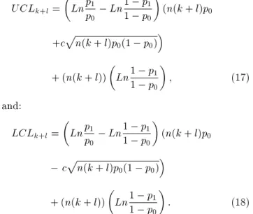
Visual basic 7 is used to compare our method with the standard np chart, Binomial EWMA, Binomial CUSUM and moving average chart. Through simula-tion, after establishing the control chart, the obtained control limits from Equations 16 and 17 are divergent and very close to each other at the beginning. It means that our interval is very tight at rst. When the process is in-control, this causes some initial data to fall to out-of-control zones immediately, and some of them to fall to out-of-control zones later. Consequently, we are faced by a very large variation of run length (VRL0).
To overcome this problem, a constant value, l, will be added to the parameter, k, as follows:
UCLk+l=
Lnpp1
0 Ln
1 p1
1 p0
(n(k + l)p0
+cpn(k + l)p0(1 p0)
+ (n(k + l))
Ln1 p1 p1
0
; (17)
and:
LCLk+l=
Lnp1
p0 Ln
1 p1
1 p0
(n(k + l)p0
cpn(k + l)p0(1 p0)
+ (n(k + l))
Ln1 p1 p1
0
: (18)
By this modication, the values of VRL0 become
smaller and the appropriate ARL0will be reached. In
other words, by using this parameter, we start at point l of the control limits instead of point zero. In the next stage, we should estimate a value for statistics, Ln(zk+l), when k = 0, the initial value of the statistics,
or the value of Ln(zl). As mentioned before, if we do
not have any information about the process, we put the initial value of B(l) equal to 0.5; l is a new value instead of zero. Furthermore, under this condition, we assume Ln(zl) at the middle of the interval (LCLl; UCLl). It
means that Ln(zl) is equal to:
0:5 (LCLl+ UCLl):
Therefore, we have:
Ln(zl) = B(l) (LCLl+ UCLl):
It is noticeable that if we guess that the fraction of nonconforming is greater than (less than) p0, then we
set a value B(l) 0:5 (B(l) 0:5). Parameter l is one of the parameters of the discussed model, and
it is dened in such a way that in combination with the dened value of c, the desired ARL0 and ARL1
is reached. Afterwards, we compare the presented method with some other methods developed in the literature.
The selected methods for comparison are binomial EWMA for = 0.02, 0.05 and 0.08 and various values of parameter A, binomial CUSUM, moving average for w = 2, 3 and 4, and the standard np control chart. Comparison of the values for parameters of the binomial EWMA and the moving average, are selected as those in Khoo [13]. The values of l and c are selected, based on the acquisition of good results for ARL0 and
standard deviation of RL0 (SDRL0).
To check the validity of our method, we generate two independent binomial distributions with parame-ters p0 = 0.1, p0 = 0.2 and n = 200. In the next
step, using Equation 10, we update belief zk. When
zk is greater than UCLk+lin Equation 18, or less than
LCLk+lin Equation 19, then, an out-of-control signal
is observed.
For the comparison study, we calculate the stock-ticker ARL1values for all considered methods by 10000
independent replications, i.e. M = 10000, for dierent values of p1, which are indicated in the rst column of
Tables 1 and 2.
The simulation results given in Tables 1 and 2 and also Figures 1 and 2, clearly show that the proposed method is better than binomial EWMA, binomial CUSUM, the moving average and standard np control chart for shifts of small magnitude from the target value, p0, but for shifts of large magnitude from the
target value, our method is not as good as the others. According to the results represented in Tables 1 and 2, the following are observed:
Figure 1. Comparison between binomial EWMA, binomial CUSUM, moving average, np chart and variable limit np control chart for p0 = 0.1 (results of EWMA and
Table 1. ARL proles for binomial EWMA, binomial CUSUM, moving average, np chart and variable limit np control chart based on p0 = 0.10 and n = 200, M=10000 computed by means of a simulation.
Binomial EWMA
Binomial CUSUM
Moving
Average np Chart
Variable Limit np Control
Chart p1 = 0.02
A = 2:1257
= 0.05 A = 2:652
= 0.08 A = 2:7650
U = 0 K = 0:1 H = 0:39
W = 2 W = 3 W = 4 C = 3
l = 120 C = 1 B(l) = 0.5 ARL SDRL ARL SDRL ARL SDRL ARL SDRL ARL SDRL ARL SDRL ARL SDRL ARL SDRL ARL SDRL
0.040 4.4 0.5 3.7 0.6 3.2 0.5 - - 1.7 0.7 1.6 0.6 1.6 0.6 2.21 1.6 4.5 0.6
0.050 5.3 0.8 4.4 0.8 3.8 0.7 - - 2.5 1.5 2.3 1 2.2 0.9 4.7 4.2 5.3 0.8
0.060 6.6 1.1 5.6 1.1 4.9 1.1 - - 5 4 3.7 2.3 3.3 1.7 12.1 11.5 6.5 1.1
0.070 8.8 1.9 7.6 2 6.8 2 - - 13.8 12.5 8.3 6.7 6.4 4.5 36.2 34.7 8.7 1.9
0.080 13.5 3.9 12.4 4.3 11.5 4.7 - - 54.8 55 29 27.3 19.5 17.6 122.8 122.3 13.2 3.7 0.085 18.7 6.5 18.1 7.9 17.6 9.1 - - 123.3 121.1 67.3 66.7 43.1 40.9 226.7 224.3 17.6 5.8 0.090 30.1 13.3 32.7 18.6 34.3 22.9 - - 284 271.6 178.2 175.5 116.6 112.9 381.2 381.3 26.9 11.3 0.095 71.8 46.3 102.7 82.8 120.2 108.3 - - 568 574.6 467.6 461 345.2 344.3 441.2 435.3 59.7 37.4 0.105 70.7 47.1 93.3 76 101.9 92.3 73.3 35.1 213.4 213.4 208 207.2 194.7 186.6 161.6 160.8 57.7 38.7 0.110 30.1 14.5 32 19.6 32.7 22.5 38.8 13.9 92.3 89.6 77.1 74.7 64.3 62.3 84.1 82.9 27.9 12.9 0.115 18.9 7.5 18.1 8.8 17.2 9.6 26.9 7.5 43 40.7 34.9 33 28.4 26 46.9 45.8 17.9 6.7 0.120 13.7 4.7 12.4 5.1 11.5 5.4 20 5 23.1 22.1 17.9 16.7 14.9 13 27.7 26.9 13.2 4.3
0.130 8.9 2.5 7.8 2.6 6.9 2.6 13.9 3 8.3 7.4 6.7 5.6 6 4.6 11.2 10.4 8.8 2.4
0.140 6.6 1.7 5.7 1.6 5 1.6 10.5 1.9 4.3 3.5 3.7 2.6 3.5 2.3 5.6 5.1 6.6 1.6
0.150 5.3 1.2 4.5 1.2 3.9 1.1 8.3 1.4 2.6 1.9 2.5 1.5 2.4 1.3 3.3 2.7 5.4 1.1
0.160 4.5 1 3.8 1 3.3 0.9 7.2 1.24 1.9 1.1 1.9 1 1.8 0.9 2.2 1.6 4.6 0.9
p0 = 0.1 390.1 392 585.3 625.9 537.7 553.6 416 342.6 496.6 495.7 549.7 564.4 556.7 535 302 302 860.5 2391.9
Figure 2. Comparison between binomial EWMA, binomial CUSUM, moving average, np chart and variable limit np control chart for p0 = 0.2 (results of EWMA and
MA are the best results shown in Table 2).
1. The initial value of zlis assumed to be 0:5 (LCLl
+ UCLl). It means that the process is in an
out-of-control state with the probability of B(l) = 0:5. We dene this initial value based on our recognition about the process, and it can have any other values in the (LCLl, UCLl) interval.
2. We dene parameters c and l to obtain the desired ARL0 and ARL1,
3. The standard deviation of RL0(SDRL0) in our
ap-proach is large in comparison with other methods; but the ARL0value is pretty large. Also, as shown
in Tables 3 and 4, the initial 10 percent of RL0in the
new method is pretty equivalent to other methods. Therefore, overall, the ARL0 in the new method is
better than the others.
4. It is noticeable that the ARL0 in the new method
Table 2. ARL proles for binomial EWMA, binomial CUSUM, moving average, np chart and variable limit np control chart based on p0 = 0.20 and n = 200, M = 10000 computed by means of a simulation.
Binomial EWMA
Binomial CUSUM
Moving
Average np Chart
Variable Limit np Control
Chart p1 = 0.02
A = 2:1257
= 0.05 A = 2:6150
= 0.08 A = 2:7650
U = 0 K = 0:1 H = 0:52
W = 2 W = 3 W = 4 C = 3
l = 120 C = 1 B(l) = 0.5 ARL SDRL ARL SDRL ARL SDRL ARL SDRL ARL SDRL ARL SDRL ARL SDRL ARL SDRL ARL SDRL
0.140 5.9 1 4.9 1 4.3 1 - - 3.2 2.3 2.8 1.5 2.6 1.3 5.5 5 5.9 1
0.150 7 1.4 5.9 1.4 5.3 1.4 - - 5.5 4.4 4.1 2.8 3.7 2.2 10.7 10.3 7 1.4
0.160 8.8 2.1 7.6 2.1 6.8 2.1 - - 11 9.7 7.4 5.9 6 4.3 21.7 21.2 8.7 1.9
0.170 11.9 3.3 10.6 3.5 9.9 3.8 - - 27.3 26.3 16.2 14.7 12.4 10.3 48.9 48.1 11.7 3 0.180 18.7 6.8 17.7 7.9 17.5 9.2 - - 80.8 81.1 48.5 47.1 35 33 121.8 121 17.5 5.7 0.185 26.1 11.3 26.5 14.8 27.6 18.2 - - 154.2 157.1 94.9 92.3 70.2 68.3 187.7 196.8 23.6 9.6 0.190 43.1 24.2 49.6 34.5 56.1 43 - - 289.6 284.6 206.1 202.7 158.1 156.1 272.4 279.7 37.9 20.5 0.195 102.6 77.6 144.8 129.8 172.7 167.6 - - 490.4 509.9 408 412.2 331.9 335.4 326.5 328.4 79.4 61.9 0.205 100.8 74.6 133.4 122.2 154.8 144.5 96.7 52.4 297.4 316.1 257.3 267.1 239.4 246.1 201.8 202 84.5 63.8 0.210 42.8 24.2 48.2 34.9 53.5 43.2 51.2 19.8 158.6 167.7 127.6 133 108.8 112.2 129 127.7 37.3 19.6 0.215 26.2 12 26.4 15.1 27 17.6 36.1 10.1 84 85.4 63.2 63.4 51.2 51.9 82.6 83.1 24.2 10.4 0.220 18.8 7.4 17.7 8.4 17.1 9.5 27.4 7.3 47.9 46.6 34.8 33.6 28.4 26.8 53.5 53.2 17.6 6.6 0.230 12 3.9 10.6 4 9.9 4.3 18.2 4.2 18.3 17.5 13.2 12 11 9.4 24.4 24.4 11.7 3.5 0.240 8.9 2.4 7.6 2.4 6.9 2.5 13.8 2.8 8.8 8 6.7 5.5 5.9 4.4 12.5 11.9 8.8 2.3
0.250 7.1 1.7 6 1.7 5.3 1.6 11.1 2 4.9 4.1 4 3 3.7 2.5 6.9 4.4 7 1.7
0.260 5.9 1.3 4.9 1.25 4.4 1.2 9.2 1.62 3.2 2.4 2.8 1.8 2.7 1.5 4.4 3.8 5.9 1.3 p0=0.2 359 348.2 496.8 515.9 490.6 498.8 400.8 329.7 475.2 481.3 460.3 459 418.1 428.7 284.2 282.8 698.9 1747.9
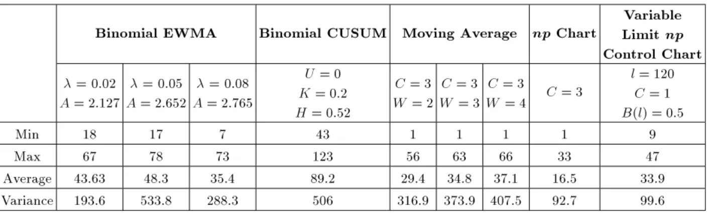
Table 3. RL0 for initial 10 percent of data (p0= 0:1, n = 200, M = 10000).
Binomial EWMA Binomial CUSUM Moving Average np Chart
Variable Limit np Control Chart = 0.02
A = 2:127
= 0.05 A = 2:652
= 0.08 A = 2:765
U = 0 K = 0:2 H = 0:52
C = 3 W = 2
C = 3 W = 3
C = 3
W = 4 C = 3
l = 120 C = 1 B(l) = 0:5
Min 18 17 7 43 1 1 1 1 9
Max 67 78 73 123 56 63 66 33 47
Average 43.63 48.3 35.4 89.2 29.4 34.8 37.1 16.5 33.9
Variance 193.6 533.8 288.3 506 316.9 373.9 407.5 92.7 99.6
deviations, compared to other considered methods in this research.
5. The standard deviation of RL1 (SDRL1) in the
variable limit control chart is usually less than its value in other methods.
6. The proposed method is eective for the control of
production processes, in which the recognition of small deviations from p0 is important, such as in
high tech processes.
7. In accordance with the gained control limits from Equations 17 and 18, it is clear that they are divergent, therefore, in the long run, our interval
Table 4. RL0 for initial 10 percent of data (p0= 0:2, n = 200, M = 10000).
Binomial EWMA Binomial CUSUM Moving Average np Chart
Variable Limit np Control Chart =0.02
A = 2:127
= 0:05 A = 2:615
= 0:08 A = 2:765
U = 0 K = 0:2 H = 0:52
C = 3 W = 2
C = 3 W = 3
C = 3
W = 4 C = 3
l = 120 C = 1 B(l) = 0:5
Min 12 10 9 35 1 1 1 1 6
Max 66 54 51 104 44 53 39 29 43
Average 42 37.9 35.4 76 21.2 22 22 14.2 29.1
Variance 223.5 101.9 101.4 338 185.9 231 139.4 61.7 98.5
Table 5. ARL sensitivity analysis for parameter B(l) (p0= 0:2, n = 200, M = 10000).
p1 B(l) = 0:5
C = 1; l = 120
B(l) = 0:55 C = 1; l = 120
B(l) = 0:6 C = 1; l = 120
B(l) = 0:65 C = 1; l = 120
0.14 5.9 6.4 6.9 7.4
0.15 7 7.7 8.2 8.9
0.16 8.7 9.6 10.3 11.1
0.17 11.7 12.7 13.8 14.8
0.18 17.5 19.2 20.7 22.3
0.185 23.6 26.5 28.1 30.3
0.19 37.9 42.3 46 49.1
0.195 79.4 85.7 94.4 101.2
0.205 84.5 75.9 66.5 59.9
0.21 37.3 34 31.4 27.2
0.215 24.2 22.1 19.8 17.6
0.22 17.6 16.2 14.5 12.6
0.23 11.7 10.5 9.3 8.5
0.24 8.8 8 7.2 6.4
0.25 7 6.5 5.7 5.1
0.26 5.9 5.4 4.8 4.4
p0 = 0.2 698.9 558.5 565.5 504.5
will be wide and the ARL1 of the control chart
is increased. Consequently, it is applicable for evaluation of the initial setup of a process.
In general, using the new method will results a better ARL0 despite showing a larger SDRL0. Also, for small
deviations from the target, the ARL1 and SDRL1 of
this approach are better than other methods. Hence, the proposed method oers a better performance under certain conditions.
In the next stage, a sensitivity analysis is per-formed for the parameters of our model. There are six parameters in our model, namely, n, c, l, p0, p1and
B(l). Based on simulation results, sensitive parameters in our model are B(l), c and l. The variations of other parameters are not eective. The sensitivity analysis for parameter B(l) is given in Table 5. Appropriate values of c and l depend on process conditions and must be evaluated properly.
Table 5 demonstrates that when the value of B(l) is increased, our method is more capable of recognizing an upward shift in the quantity of nonconforming (p1>
p0), and vice-versa. Also, for fair comparison, we used
other good values for parameters of Binomial EWMA and Binomial CUSUM, the results of which are shown in Tables 6 and 7.
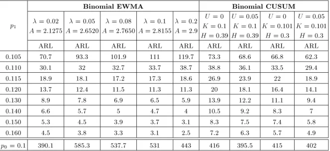
Table 6. Other simulation results for binomial EWMA and binomial CUSUM (p0= 0:1, n = 200, M = 10000).
Binomial EWMA Binomial CUSUM
p1 = 0.02
A = 2:1275
= 0.05 A = 2:6520
= 0.08 A = 2:7650
= 0.1 A = 2:8155
= 0.2 A = 2:9
U = 0 K = 0:1 H = 0:39
U = 0:05 K = 0:1 H = 0:39
U = 0 K = 0:101
H = 0:3
U = 0:05 K = 0:101
H = 0:3
ARL ARL ARL ARL ARL ARL ARL ARL ARL
0.105 70.7 93.3 101.9 111 119.7 73.3 68.6 66.8 62.3
0.110 30.1 32 32.7 33.7 38.7 38.8 36.1 33.5 29.4
0.115 18.9 18.1 17.2 17.3 18.6 26.9 23.9 22 18.9
0.120 13.7 12.4 11.5 11.3 11.3 20 18.1 16.4 14.1
0.130 8.9 7.8 6.9 6.5 5.9 13.9 12.2 11.1 9.4
0.140 6.6 5.7 5 4.7 4 10.5 9.2 8.3 7
0.150 5.3 4.5 3.9 3.7 3.1 8.3 7.5 7.4 5.8
0.160 4.5 3.8 3.3 3.1 2.5 7.2 6.3 5.7 4.9
p0 = 0.1 390.1 585.3 537.7 531 443 416 395.5 415 402
Table 7. Other simulation results for binomial EWMA and binomial CUSUM (p0= 0:2, n = 200, M = 10000).
Binomial EWMA Binomial CUSUM
p1 = 0:02
A = 2:1275
= 0:05 A = 2:6150
= 0:08 A = 2:7650
= 0:1 A = 2:84
= 0:2 A = 2:9
U = 0 K = 0:2 H = 0:52
U = 0:05 K = 0:2 H = 0:52
U = 0 K = 0:201
H = 0:45
U = 0:05 K = 0:201
H = 0:45
ARL ARL ARL ARL ARL ARL ARL ARL ARL
0.205 100.8 133.4 154.8 170.4 175.4 96.7 90.9 95.8 91.5
0.210 42.8 48.2 53.5 58.9 67.4 51.2 49.2 49 45.4
0.215 26.2 26.4 27 28.5 31.6 36.1 33.1 32.6 29.9
0.220 18.8 17.7 17.1 17.6 18.1 27.4 25 24.4 22.2
0.230 12 10.6 9.9 9.5 8.9 18.2 16.8 16.4 14.6
0.240 8.9 7.6 6.9 6.6 5.8 13.8 12.5 12.3 11
0.250 7.1 6 5.3 5.1 4.4 11.1 10.2 9.9 8.8
0.260 5.9 4.9 4.4 4.2 3.4 9.2 8.5 8.3 7.5
p0=0.2 359 496.8 490.6 508 391 400.8 385.6 430.4 427.3
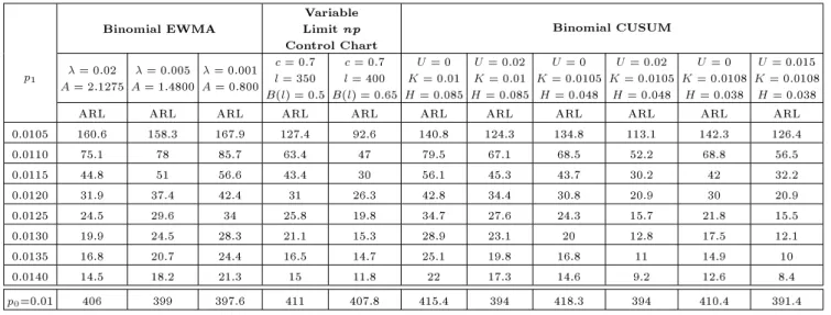
Also, for low values of p1 that are related to high
tech processes, Table 8 demonstrates that our method is superior to others.
As clear from Tables 6 to 8, the results of ARL1
related to the proposed control chart are better than the best results of Binomial EWMA and Binomial CUSUM.
NUMERICAL EXAMPLE
In this section, we describe our methodology step by step as follows.
1. Input l; B(l); c; n; p0and p1,
2. For k = 0 : m,
3. Calculate LCLk+l and UCLk+l,
4. End,
5. Set Ln(zl) = B(l)(LCLl+ UCLl),
6. For k = 1 : m,
7. Determine Xk and Ln(zk+l),
8. If LCLk+l Ln(zk+l) UCLk+l,
9. The process is in-control, 10. Else,
11. The process is out-of-control and makes an alarm, 12. Check the process and perform corrective action, 13. Go to step 3,
14. End, 15. End.
Table 8. Simulation results for binomial EWMA, binomial CUSUM and variable limit np control chart (p0= 0:01,
n = 500, M = 10000).
Binomial EWMA Limit npVariable Control Chart
Binomial CUSUM p1 = 0:02
A = 2:1275
= 0:005 A = 1:4800
= 0:001 A = 0:800
c = 0:7 l = 350 B(l) = 0:5
c = 0:7 l = 400 B(l) = 0:65
U = 0 K = 0:01 H = 0:085
U = 0:02 K = 0:01 H = 0:085
U = 0 K = 0:0105
H = 0:048
U = 0:02 K = 0:0105
H = 0:048
U = 0 K = 0:0108
H = 0:038
U = 0:015 K = 0:0108
H = 0:038
ARL ARL ARL ARL ARL ARL ARL ARL ARL ARL ARL
0.0105 160.6 158.3 167.9 127.4 92.6 140.8 124.3 134.8 113.1 142.3 126.4
0.0110 75.1 78 85.7 63.4 47 79.5 67.1 68.5 52.2 68.8 56.5
0.0115 44.8 51 56.6 43.4 30 56.1 45.3 43.7 30.2 42 32.2
0.0120 31.9 37.4 42.4 31 26.3 42.8 34.4 30.8 20.9 30 20.9
0.0125 24.5 29.6 34 25.8 19.8 34.7 27.6 24.3 15.7 21.8 15.5
0.0130 19.9 24.5 28.3 21.1 15.3 28.9 23.1 20 12.8 17.5 12.1
0.0135 16.8 20.7 24.4 16.5 14.7 25.1 19.8 16.8 11 14.9 10
0.0140 14.5 18.2 21.3 15 11.8 22 17.3 14.6 9.2 12.6 8.4
p0=0.01 406 399 397.6 411 407.8 415.4 394 418.3 394 410.4 391.4
Table 9. Obtained values for LCLk+l, UCLk+l, Xk and Ln(zk+l) for mentioned case study when process is in-control.
l = 120; B(l) = 0:5; c = 1; n = 200; p0 = 0:1; p1= 0:12
k 0 1 2 3 4 5 6 7 8 9
LCLk+l -15.0 -15.1 -15.3 -15.4 -15.5 -15.7 -15.8 -15.9 -16.0 -16.2
UCLk+l -6.0 -6.1 -6.1 -6.2 -6.3 -6.4 -6.5 -6.6 -6.6 -6.7
Xk - 20 16 15 22 15 23 18 20 15
Ln(zk+l) -10.5 -10.6 -11.1 -11.8 -11.7 -12.3 -12.1 -12.4 -12.5 -13.1
In the above algorithm, m is the number of subgroups that will be observed from the process. As mentioned before, the best values for l and c are 120 and 1, respectively. For example, assume that l = 120, c = 1, n = 200, p0= 0.1 and p1 = 0.12. Also, assume
that the number of subgroups, m, is 10. Obtained values for LCLk+l, UCLk+l, Xk and Ln(zk+l) are
shown in Table 9.
The drawing of control limits for the above infor-mation is shown in Figure 3. As observed from Table 9 and Figure 3, at rst the control limits are divergent and then they have a negative gradient.
CONCLUSIONS
In this research, we applied an initial belief to detect the out-of-control state in the np attribute control charts, and since this approach analyzes data sequen-tially, it has demonstrated a very good performance. It has been found that, in general, the variable limit control np charts are able to improve the eectiveness of detecting shifts in p0 to a substantial degree,
es-pecially for the small shifts in p0, without increasing
the false alarm rate. Although the cost of running variable limit control np charts is relatively high, the
Figure 3. Control limits for Ln(zk+l) based on
information shown in Table 9.
use of these charts can be justied by the signicant improvement in their performance. In general, the proposed method yields a signicant improvement in ARL0 and, for small deviations of the process, it
improves ARL1.
For future research, we propose considering other functions to dene the beliefs and economic design of parameters using this approach.
REFERENCES
1. Vargas, V., Lopes, L. and Souza, A. \Comparative study of the performance of the CUSUM and EWMA control charts", Computers & Industrial Engineering, 46, pp. 707-724 (2004).
2. Zhang, S. and Wu, Z. \Designs of control charts with supplementary runs rules", Computers & Industrial Engineering, 49, pp. 76-97 (2005).
3. Woodall, W.H. \Control charts based on attribute data: Bibliography and review", Journal of Quality Technology, 29, pp. 172-184 (1997).
4. Montgomery, D.C., Introduction to Statistical Quality Control, Wiley, New York (2002).
5. Reynolds, M. and Stoumbos, Z. \A CUSUM chart for monitoring a proportion when inspecting continu-ously", Journal of Quality Technology, 31, pp. 87-109 (1999).
6. Gan, FF. \An optimal design of CUSUM control charts for binomial counts", Journal of Applied Statistics, 20, pp. 445-460 (1993).
7. Roberts, S.W. \Control chart tests based on geomet-ric moving averages", Technometgeomet-rics, 1, pp. 239-250 (1959).
8. Hunter, J.S. \The exponentially weighted moving av-erage", Journal of Quality Technology, 18, pp. 203-210 (1986).
9. Crowder, S.V. \Computation of ARL for combined individual measurement and moving range charts", Journal of Quality Technology, 19, pp. 98-102 (1987a). 10. Crowder, S.V. \A simple method for studying run-length distributions of exponentially weighted mov-ing average charts", Technometrics, 29, pp. 401-407 (1987b).
11. Lucas, J.M. and Saccucci, M.S. \Exponentially weighted moving average control schemes: Proper-ties and enhancements", Technometrics, 32, pp. 1-29 (1990).
12. Somerville, S.E., Montgomery, D.C. and Runger, G.C. \Filtering and smoothing methods for mixed particle count distributions", International Journal of Produc-tion Research, 40, pp. 2991-3013 (2002).
13. Khoo, M. \A moving average control chart for mon-itoring the fraction of nonconforming", Quality and Reliability Engineering International, 20, pp. 617-635 (2004).
BIOGRAPHIES
Mohammad Hossein Abooie is a faculty member of the Industrial Engineering group at Yazd University in Iran. He obtained his BS, MS and PhD in Industrial Engineering from Amirkabir University in Tehran, Iran. His current research interests include: Statistical Process Control and Application of Statistics to Indus-trial problems.
Majid Aminnayeri received his BS in Mathematics and MS in Mathematical Statistics from Pahlavi Uni-versity in 1973 and 1975, respectively. His PhD, double majoring in Statistics and Industrial Engineering, was awarded to him by Iowa State University in 1981 and he served as a faculty member of Kerman University from 1982 to 1989. Since 1991, he has been with Amirkabir University of Technology, AUT, in which, from 1993 to 1997, he has served as Chairman of the Industrial Engineering Department.
Dr Aminnayeri is working in SPC, Scheduling, as well as Stochastic Modeling. He has much experience in applying theory to practice, and in this regard, three important projects that he has been involved in are: the 1986 Iranian Census, the 1993 Tehran OD study, and, in 1994, the Estimation of the Number of Running Motorcycles in Tehran Project.
Dr Aminnyaeri has publications in ISI journals as well as international conference papers.