A
Watershed’s
Hydrologic
Response
after a
Forest Fire
Team Fireshed Capstone 2013
Binyu Wang Garrett Freer Kristie Marriott
1 | P a g e
TABLE OF CONTENTS
SECTION 1 #
SECTION 1.1 #
SECTION 1.2 #
SECTION 1.3 #
CHAPTER 2 #
SECTION 2.1 #
SECTION 2.2 #
SECTION 2.3 #
CHAPTER 3 #
SECTION 3.1 #
SECTION 3.2 #
2 | P a g e
I. PROJECT UNDERSTANDING ... 4
II. BACKGROUND ... 4
A. THE NEED FOR FOREST RESTORATION ... 4
B. TYPES OF FOREST MANAGING/FUEL TREATMENTS ... 4
C. FOREST DENSITY AND FIRE SEVERITY ... 5
III. CHALLENGES ... 6
A. BURN SEVERITY ... 6
B. HYDROLOGIC RESPONSE TO FIRES ... 6
IV. SCOPE OF SERVICES ... 8
A. TASK 1-PROJECT MANAGEMENT ... 8
1. 1.1GROUP MEETING ... 8
2. 1.2TECHNICAL MEETING ... 8
B. TASK 2-PROJECT PROPOSAL DEVELOPMENT ... 9
1. 2.1DEVELOP PROJECT UNDERSTANDING ... 9
2. 2.2DEVELOP SCOPE OF SERVICES ... 9
3. 2.3TASK TIMELINE ... 9
4. 2.4TASK STAFFING ... 9
5. 2.5BUDGET ... 9
C. TASK 3-DETERMINATION OF WATERSHED CHARACTERISTICS ... 10
1. 3.1LOCATION ... 10
2. 3.2ANNUAL PRECIPITATION ... 10
3. 3.3WATERSHED CONDITIONS ... 10
D. TASK 4-HYDROLOGICAL RESPONSE ... 10
1. 4.1REVIEW EXISTING LITERATURE ... 10
2. 4.2DETERMINE CURRENT CONDITIONS ... 10
3. 4.3EVALUATE CURRENT CONDITIONS WITH RESPECT TO EXISTING LITERATURE 10 4. 4.4ECOLOGICAL RESPONSE TO THINNING ... 11
E. TASK 5-POST THINNING EVALUATION ... 11
1. 5.1HEC-HMSMODELING ... 11
F. TASK 6-PROJECT STUDY REPORT ... 11
1. 6.1REPORT PREPARATION ... 11
2. 6.2FINAL PROJECT STUDY REPORT ... 11
3. 6.3PRESENTATION ... 11
4. 6.4WEBSITE ... 11
V. TIMELINE ... 12
VI. STAFFING PLAN ... 13
VII. BUDGET ... 15
VIII. WATERSHED- 1.0 ... 17
A. CHARACTERISTICS -1.1 ... 17
3 | P a g e
1. HYDRODESKTOP -1.2.1 ... 17
C. MEASUREMENTS AND CALCULATIONS -2.0 ... 20
1. SLOPE CALCULATIONS -2.1 ... 20
2. LAG TIME AND TIME OF CONCENTRATION-2.2 ... 21
3. FLOW (Q)CALCULATIONS ... 22
IX. HEC-HMS 3.5 ... 23
A. OVERVIEW ... 23
1. WATERSHED PHYSICAL DESCRIPTION ... 23
2. METEOROLOGY DESCRIPTION ... 24
3. HYDROLOGIC SIMULATION ... 25
4. PARAMETER ESTIMATION ... 26
5. ANALYZING SIMULATIONS ... 26
6. GISCONNECTION ... 26
7. BASIN MODELS ... 26
8. SUBBASIN ELEMENTS ... 27
9. HYDROLOGICAL ELEMENTS ... 27
10. PROJECT WATERSHED MODEL ... 28
11. PRECIPITATION METHOD ... 29
12. SELECTING A LOSS METHOD ... 30
13. SELECTING A ROUTING AND TRANSFORM METHOD ... 31
14. SCSCURVE NUMBER LOSS ... 31
15. GREEN AND AMPT LOSS ... 31
4 | P a g e
P
ARTA
I.
Project Understanding
The purpose of this project is to conduct watershed modeling of northern Flagstaff. These watershed models will depict the consequences of a forest fire. The purpose of the watershed modeling is to try and determine the amount of runoff which will occur when taking into account several factors. We will look at fire intensity and how it relates to burn severity, and how fuel loading can be changed by mechanical thinning. We will communicate how we believe the hydraulic response will be if encountering a catastrophic fire, and how this relates with different levels of thinning. Finally, we will lay out different treatment methods and how these will affect burn severity and hydraulic response. We will use Digital Elevation Models (DEM), GIS, Water Erosion Predictions (WEP), and other programs such as HEC-HMS in order to model different scenarios containing the above mentioned factors.
II.
Background
A.
The Need for Forest Restoration
There is a need to improve forest health across Arizona. The lack of diversity and the
diminishing forest health have resulted in a forest that is less resilient to damage caused by drought, insect outbreaks, climate change, and intense wildfires. The accumulation of large amounts of ground fuels, dense tree growth, interlocking tree crowns, a combination of climate change and reduced water shed, create conditions for intense devastating, high intensity crown fires. These crown fires destroy forest along with ecosystem, and wildlife habitats. To help improve forest health and decrease the chances of a high burn intensity fire, treatments have been designed to manage mature trees. Forest management is accomplished by cutting and removing younger small diameter trees. This process of removing the younger trees will help sustain and manage older trees and provides a much older mature forest structure, and helps reduce the effect of a wildfire on the landscape.
B.
Types of Forest Managing/ Fuel Treatments
There are at least three ways to reduce tree densities and accomplish fuel treatment: wildfire, prescribed fire and mechanical thinning. The first, reliance on wildfires, is impractical. Letting natural fires play their historical role may have unwanted effects in forests that have
undergone major stand structural changes over the past years of fire exclusion. In many ponderosa pine forests choked with dense, small-diameter trees, or encroached by shade-tolerant trees, natural fires may no longer play a strategic role (Omni).
5 | P a g e
The second strategy for restoring these forests is large-scale prescribed burning. This is likely to be effective in stands that have moderate or low tree densities, little encroachment of ladder fuels, moderate to steep slopes which preclude mechanical treatment, and expertise in
personnel to plan and implement such large prescribed burns. Large-scale implementation of this strategy will require funding for the planning and implementation over current
expenditures and may require modifications to current air quality legislation (Omni).
Mechanical tree removal, the third strategy, works best on forests that are too densely packed to burn, that have nearby markets for small-diameter trees, and areas where expertise and personnel
are not available for prescribed burning programs. Mechanical tree removal may be
accomplished by many different types of harvest, including pre-commercial thinning, selection or shelter wood harvest coupled with small-diameter tree removal, and thinning from below. The goal is to manage forests for much lower tree densities leaving larger residual trees. Harvests to reduce wildfire hazard will remove small-diameter trees in contrast to traditional timber harvests. Mechanical fuel treatments can be very labor intensive, especially on steep slopes and in remote areas, and may not be commercially attractive due to the small diameter trees that need removal. To make fuel treatments more cost-effective for small-diameter trees, consistent markets are necessary (Omni).
C.
Forest Density and Fire Severity
Numerous recent studies have concluded that some type of fuel treatment results in less severe wildfires. Different levels and types of fuel treatments, also known as forest thinning, result in a forest with much lower density and larger trees. Stands with fewer trees have less continuous crown and ladder fuels. Larger trees generally have crowns higher off the ground and have thicker bark which makes them more fire resistant. This two-fold benefit of treated stands, results in a lower potential for crown fire initiation, propagation, and for less severe fire effects. A recent study looked at aspects of stand structure that affect changes in fire severity since previous studies have inferred that fuel treatment resulting in stand structure manipulations mitigate fire hazard. To determine the fuel treatment’s effect on stand characteristics, three variables describing stand structure were measured: stand density (trees/hectare), basal area (meters2/hectare) and average diameter (cm) of trees on the plot. Crown characteristics, such as crown weight and height to live crown, were also measured since they are known to drive crown fire behavior (Van Wagner 1977, Rothermel 1991). To measure fire effects, one rating of fire severity at each plot and percent crown scorch for each tree on the plot was recorded. Fire
6 | P a g e
severity was classified by observing foliage scorch and crown needle consumption (Wagener 1961, Wyant 1986). The following criteria were used to determine fire severity:
Unburned, fire did not enter the stand
Light, surface burn without crown scorch
Spotty, irregular crown scorch
Moderate, intense burn with complete crown scorch
Severe, high intensity burn with crowns totally consumed
The results from the study showed the treated plots in this study have lower fire severity ratings and less crown scorch than the untreated plots. From these results we infer that the types of fuel treatments studied reduce fire severity rating and crown scorch. The treated plots burned less severely in terms of below-ground fire severity. Based on the statistical results and field reconnaissance, sites with mechanical fuel treatment appear to have more dramatically reduced fire severity compared to sites with prescribed fire only. Although fire severity ratings and percent crown scorch are lower at treated plots and higher at untreated plots at all sites (Omni & Pollet).
III. Challenges
A.
Burn Severity
Burn severity is a function of physical and ecological changes caused by fire. Fires burn heterogeneously across landscapes, with unburned and lightly burned patches interspersed among severely burned patches, due to variability in weather and landscape patterns. ). Fire spread and severity have been associated with abiotic factors including weather, moisture and slope. Severity can also be highly influenced by biotic conditions including tree size, succession stage and pathogens. Mapping of burn severity provides information to target recovery
activities efficiently. Large burned patches may negatively impact wildlife nesting and browsing. Vegetation mortality changes water loss through evapotranspiration, surface flow and subsurface flow. High severity burns often increase hydrophobic soil conditions, leading to increased runoff and erosion compared to less severely burned areas Unburned and low burn areas are seed sources for more severely impacted areas, which usually have fewer surviving and re-sprouting individuals ( Cocke, Fulé, & Crouse, 2005).
B.
Hydrologic Response to Fires
Forested watersheds are some of the most important sources of water supply in the world. Maintenance of good hydrologic condition is crucial to protecting the quantity and quality of stream flow on these important lands. Wildfires have the greatest potential to change
7 | P a g e
watersheds. Wild fires influence many forest ecosystems in the world depending and plays a role of variable significance depending on climate, fire frequency, and geomorphic conditions. This is particularly true in regions where high severity fire, steep terrain, high fuel loads, and post-fire seasonal precipitation interact to produce dramatic impacts (Neary, Koestner &Youberg, 2011).
“Watershed condition or the ability of a catchment system to receive and process precipitation without ecosystem degradation is a good predictor of the potential impacts of fire on water and other resources (such as roads, recreation facilities, riparian vegetation, and so forth). The surface cover of a watershed consists of the organic forest floor, vegetation, bare soil, and rock. Disruption of the organic surface cover and alteration of the mineral soil by wildfire can
produce changes in the hydrology of a watershed well beyond the range of historic variability. Low severity fires rarely produce adverse effects on watershed condition, but high severity fires usually do. Most wildfires are a chaotic mix of severities, but in parts of the world, high severity is becoming a dominant feature of fires since about 1990. Successful management of watershed resources and human populations in a post-wildfire environment require an understanding of the changes in watershed condition and hydrologic responses induced by fire. Flood flows, are the largest hydrologic response and most damaging to many natural and cultural resources” (Neary, Koestner &Youberg, 2011).
Climate change in combination with human intervention and the lack of forest management significantly increase forest fire hazard. Thus, wildfires have emerged as increasingly dominant drivers of ecosystem functioning. This has led to a new awareness about the effects of forest fires, not only in terms of vegetation loss, but also of probable loss of life and property, as well as of changes in the hydrological response. Several studies have pointed out the impact of forest fires on the hydrological cycle, including reduced infiltration rates, reduced
evapotranspiration rates and increased overland flow.
Such impact is mainly attributed to the destruction of the vegetation cover and the consequent direct influence on interception, evapotranspiration and overland flow velocity. However, forest fires can also affect hydrological processes indirectly, altering the hydraulic properties of the soil. Fires destroy the top soil organic matter destabilizing the soil structure, and they convert the organic ground cover to soluble ash, and give rise to phenomena such as water repellency. Water repellency is an abnormality in soils, which results from the coating of soil particles with organic substances reducing the affinity shown by the soil for water.
Fire impact on hydrological processes is normally apparent for one or two years after the wildfires. However, in dry areas like Flagstaff, much higher runoff and erosion rates are being noticed even five to ten years after the fire. The period necessary for the hydrological process
8 | P a g e
recovery to the pre-fire conditions greatly depends on the rate of vegetation recovery. Previous studies have shown that the period necessary for runoff and soil erosion to return to
background levels depends on the type of species existing prior to fire, because each species has its own specific recovery rate. It has also been found that the amount of litter and
vegetation cover is a key factor in reducing post-fire runoff and erosion, and in accelerating the recovery time of burned soils however, in dry areas, water shortage can seriously limit plant growth rate. The plant recovery and the recovery of post-fire hydrological responses may be constrained by factors, which are common in Flagstaff, such as harsh meteorological and hydrological conditions, plant communities with low regeneration potential that have colonized abandoned fields. South-facing slopes have also been reported as particularly sensitive to wildfire impact highlighting the vast spatial and temporal variability.
Pending your response, our team is ready to start collecting data for analyses of this project. The time frame for our full analyses should be no later than December 2013.
IV.
Scope of Services
The order of our primary tasks is listed below: Task 1- Project Management
Task 2- Project Proposal Development
Task 3- Determination of Watershed Characteristics Task 4- Hydrological Response
Task 5- Post Thinning Evaluation Task 6- Project Study Report
A.
Task 1- Project Management
1. 1.1 Group Meeting
The NAU watershed modeling team will meet to do the primary forum for researching the project early in the semester. For the rest of spring semester 2013, team meetings will be focused on testing and building models. Meeting hours are set for every Friday afternoon. All team members are required to attend.
Deliverable: Meeting Agenda, Minutes.
9 | P a g e
The NAU watershed modeling team will prepare a schedule for several meetings with technical advisor Dr. Paul Trotta in order to discuss and solve specific project needs and issues. The meeting minutes will be documented.
Deliverable: Meeting agenda, professional help on tasks. Document of guidance will be provided.
B.
Task 2- Project Proposal Development
The NAU watershed modeling team will study the hydrology of the lower Shultz Creek
Watershed in Flagstaff, Arizona. The first step is to determine the monthly water budget in the watershed by using a geographic system, ARC GIS, to integrate watershed characteristics and hydrological data. The second one is to determine the magnitude of event-based peak
discharges under disturbance scenarios from severe wildfire thinning and under current conditions.
1. 2.1 Develop Project Understanding
The team will research the project scope providing all necessary background information. The team will identify all major areas of interest. The team will produce a hard copy of the
document. The document will be provided to the client and the technical advisor. Deliverable: Technical Understanding
2. 2.2 Develop Scope of Services
The team will provide a list of task that will be completed at the end of the project. Larger tasks will be divided into sub-task. Each task and sub-task will be defined by necessary requirements for completion.
Deliverable: Task List
3. 2.3 Task Timeline
Team with develop an up to date timeline displaying the proposed project tasks and dates of completion.
Deliverable: Timeline of tasks.
4. 2.4 Task Staffing
Team will develop a staffing plan describing which team members will be working on which tasks. This staffing plan correlates with the task timeline.
Deliverable: Table displaying which team members will be responsible for which tasks.
5. 2.5 Budget
10 | P a g e
Deliverable: Budget table displaying all engineering costs for proposed project.
C.
Task 3- Determination of Watershed Characteristics
Team will be finding all watershed model input data for this task.
1. 3.1 Location
The location of this project is north of Flagstaff at lower Shultz. It is the area of land SW of the past Shultz fire.
Deliverable: Topographic map of location of proposed project.
2. 3.2 Annual Precipitation
The discharge from the watershed is based on precipitation, infiltration, evaporation, and transportation.
Deliverable: Data tables of precipitation conditions.
3. 3.3 Watershed Conditions
The cover in the watershed canopy has impact on the infiltration in the catchment. Therefore, the cover includes soil and density of the forest, including any forest restoration.
Deliverable: Topographic map, soils analysis of infiltration, green and amp method analysis.
D.
Task 4- Hydrological Response
Forest fires have impact on the hydrological cycle, including reduced infiltration rates, reduced evapotranspiration rates and increased overland flow. Fire impact on hydrological processes is normally apparent for one or two years after the wildfires. However, in dry areas like Flagstaff, much higher runoff and erosion rates are being noticed even five to ten years after the fire.
1. 4.1 Review Existing Literature
Team will look at existing reports and studies, especially the past Shultz fire. We will review the pre and post fire condition at Timberline
Deliverable: Design alternatives for best geographic system.
2. 4.2 Determine Current Conditions
Team will research the current conditions of the watershed and define any key characteristics which will benefit the input data for the modeling process.
Deliverable: Memo describing conditions.
11 | P a g e
Team will correlate existing conditions of watershed with respect to other previous defined projects.
Deliverable: Technical Memorandum.
4. 4.4 Ecological Response to Thinning
Team will evaluate what ecological responses will be when introduced to mechanical thinning of vegetation based on literature reports. This will help to predict responses in Shultz
watershed.
Deliverable: Memo reporting responses of environment due to thinning.
E.
Task 5- Post Thinning Evaluation
1. 5.1 HEC-HMS Modeling
After obtaining all the information described above, our group will determine and build watershed models. We will test the models and analyze the models based on different
scenarios. Team will model current conditions, post-fire with no treatment(s), post-fire with treatment(s), and pre-fire with treatment(s).
Deliverable: Provide alternative baseline models for existing conditions.
F.
Task 6-Project Study Report
1. 6.1 Report Preparation
Our group will prepare a draft of the project study report. The draft will document the purpose of the project, describe the model and alternatives, analyze the results, and summarize our findings. The draft will be provided to Mr. Runyon for comments and markups.
Deliverables: Draft project study report
2. 6.2 Final Project Study Report
Our group will update the project study report and provide a final project study report, based on client’s comments.
Deliverable: Final Project Study Report
3. 6.3 Presentation
Team will prepare presentation for client and NAU faculty. Deliverable: Project Presentation.
12 | P a g e
Team will develop a webpage that displays the watershed data, analysis results, and model outputs.
Deliverable: Website for proposed project.
V.
Timeline
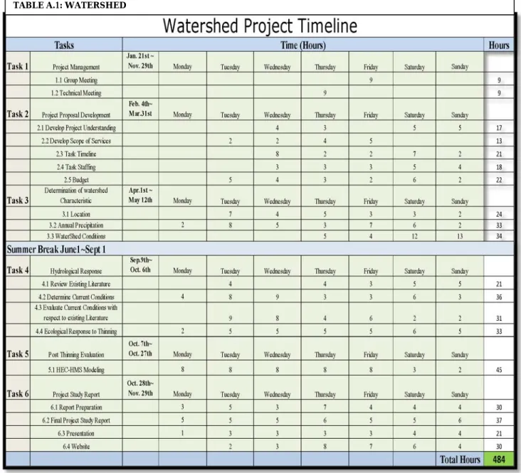
Table A.1 below displays the teams estimated time that will be allocated to each task. The tasks are broken down into sub-task to make each one more manageable.
13 | P a g e
TableA. 1 is a breakdown of the teams projected timeline. Each task has been set to be completed during a specific time period. The hours for each sub-task can be found in the individual columns. The total hours for each time period are shown in the far right column. The total hours for the entire project have been estimated to be 484 hours. The project will not be worked on by the team during the summer break.
VI.
Staffing Plan
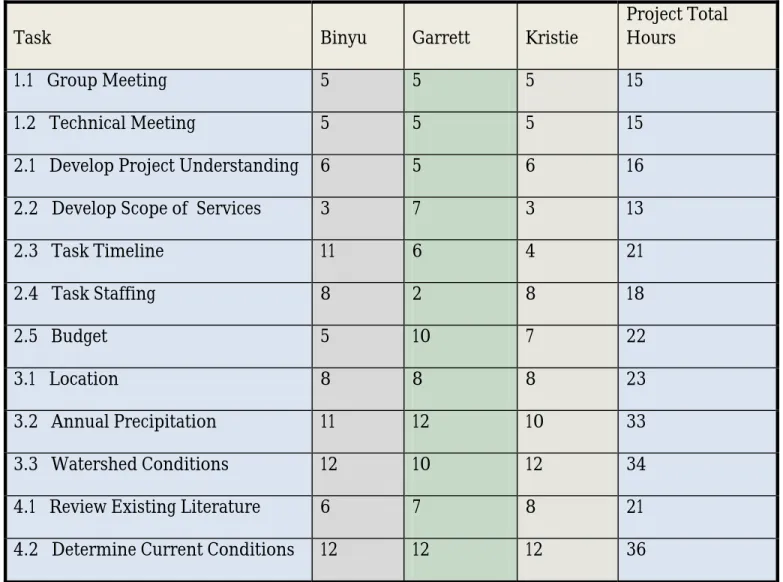
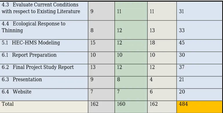
Table A.2 below is a breakdown of the individual team member that will be working on each task and the estimated hours the team member will spend on the specific task.
TABLE A. 2: TEAM STAFFING PLAN
Task Binyu Garrett Kristie
Project Total Hours
1.1 Group Meeting 5 5 5 15
1.2 Technical Meeting 5 5 5 15
2.1 Develop Project Understanding 6 5 6 16
2.2 Develop Scope of Services 3 7 3 13
2.3 Task Timeline 11 6 4 21
2.4 Task Staffing 8 2 8 18
2.5 Budget 5 10 7 22
3.1 Location 8 8 8 23
3.2 Annual Precipitation 11 12 10 33
3.3 Watershed Conditions 12 10 12 34
4.1 Review Existing Literature 6 7 8 21
14 | P a g e
4.3 Evaluate Current Conditions
with respect to Existing Literature 9 11 11 31
4.4 Ecological Response to
Thinning 8 12 13 33
5.1 HEC-HMS Modeling 15 12 18 45
6.1 Report Preparation 10 10 10 30
6.2 Final Project Study Report 13 12 12 37
6.3 Presentation 9 8 4 21
6.4 Website 7 7 6 20
Total 162 160 162 484
Table A.2 shows the amount of hours that each team member will spend working on each specific task/sub-task. The hours spent on each task by each team member can be found under the team member’s name, with their total number of hours shown in the bottom row of Table 2. The total number of hours for the entire team is 484 hours and is highlighted in the bottom right corner of Table A.2.
15 | P a g e
VII.
Budget
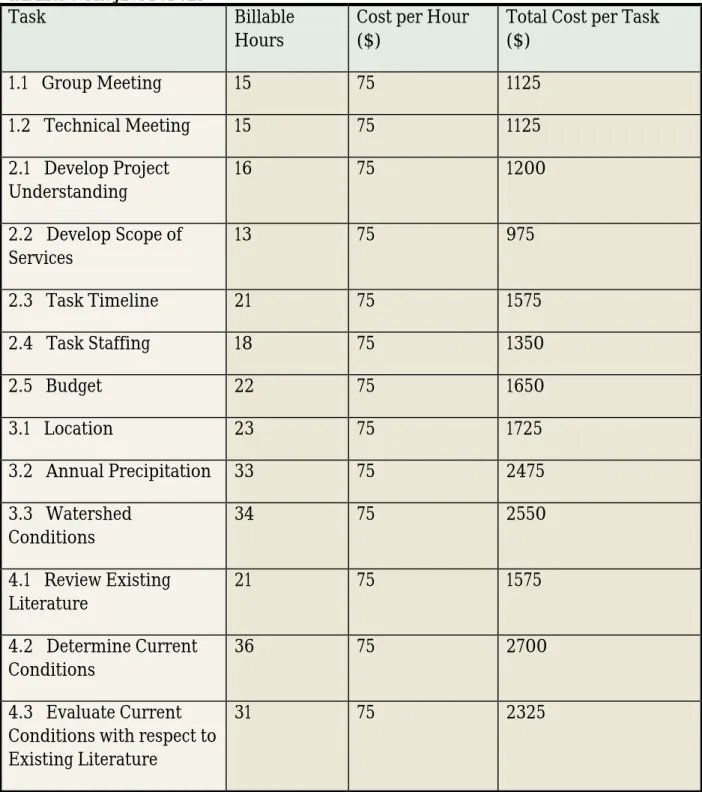
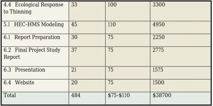
Table A. 3 below displays the total number of billable hours for each sub-task and the dollar amount the team will be charging to complete the task.
TABLE A. 3: PROJECT BUDGET
Task Billable
Hours
Cost per Hour ($)
Total Cost per Task ($)
1.1 Group Meeting 15 75 1125
1.2 Technical Meeting 15 75 1125
2.1 Develop Project Understanding
16 75 1200
2.2 Develop Scope of Services
13 75 975
2.3 Task Timeline 21 75 1575
2.4 Task Staffing 18 75 1350
2.5 Budget 22 75 1650
3.1 Location 23 75 1725
3.2 Annual Precipitation 33 75 2475
3.3 Watershed Conditions
34 75 2550
4.1 Review Existing Literature
21 75 1575
4.2 Determine Current Conditions
36 75 2700
4.3 Evaluate Current Conditions with respect to Existing Literature
16 | P a g e
4.4 Ecological Response to Thinning
33 100 3300
5.1 HEC-HMS Modeling 45 110 4950
6.1 Report Preparation 30 75 2250
6.2 Final Project Study Report
37 75 2775
6.3 Presentation 21 75 1575
6.4 Website 20 75 1500
Total 484 $75-$110 $38700
Table A.3 shows the billable hours that have been assigned to each task and the amount that will charge for the specific task. The average cost per task is $75 per hour, with some task costing $110 per hour. The cost is based on the individual task requirements and complexity. The total number of billable hours matched the total hours on the timeline and staffing plan with 484 hours. The total cost for the project is projected to be $38,700.
17 | P a g e
Part B
Final Report
VIII.
Watershed- 1.0
A.
Characteristics - 1.1
The area of interest, also known as the point of contact, falls within the Rio De Flag Watershed. The Rio De Flag is a tributary of the San Francisco Wash, which feeds into the Colorado River. It originates on the southwestern slopes of the San Francisco Mountain, and north of Flagstaff. The Rio De Flag flows over multiple terrains from flat meadows to steep rocky canyons. The elevation of the drainage area ranges from 6,800 feet to 12,356 feet. The watershed area or the complete drainage area is 2.590 square kilometers or approximately 116 square miles. The point of concentration for this project is just north of Flagstaff, near Thorp Park.
Approximately, one third of all the water contained in the Rio De Flag drains through the point of concentration. The area of the area of interest is approximately watershed is 50 square miles or 130 square kilometers.
B.
Delineation- 1.2
The team decided not to delineate the watershed by hand. The watershed was delineated using 2 different software programs. Hydrodesktop 1.5.12 was used to for the majority of the project. Near the end of the project, ArcGIS was used to check slopes and area of sub basins. The spatial analysis tool for ArcGIS is needed for any form of watershed analysis, was not available to the team until late into the project. Hydrodesktop was used as the main analysis software for the project. The software delineated sub basins were visually checked to ensure the boundary lines of all the sub basins were perpendicular to the contour lines on the topography map.
1. Hydrodesktop -1.2.1
Hydrodesktop version 1.5.12 was used to delineate the watershed, measure the areas of each sub basin, and calculate the average slope of each sub basin. A map of the United States was provided as the starter map. The area of interest was found by zooming in on the map. Once the area of interest was within the window extents a topographic map was added in the
18 | P a g e
Specific data was added to the map for a visual aid. A hydro-overlay with all bodies of water was added. The overlay made it easier to see the individual flow lines of the watershed. After all necessary data (maps and overlay) were added the points were chosen to separate the watershed into sub basins also known as catchments. Starting at the top of the watershed and working down, produced the best results. This method prevented the sub basins from
overlapping. A point on a flow line was chosen, then the “delineate” button was clicked on and the software determined all flows that contribute to that specific point. Choosing the point allowed the user to adjust each catchment in size if desired. The size of each catchment was left up to the user. Larger areas could be broken down into smaller more manageable areas by choosing a point higher in the sub basin, which reduces the size of that particular basin. The entire watershed was first delineated and a total of 28 sub basins and a total Area of 300.26 square kilometers (116 square miles). A large portion of the watershed fell below the point of concentration. The area below the point of concentration would not be used for the analysis and therefore was disregarded. FigureB.1.1 below is a screenshot of the complete watershed after it had been delineated using Hydrodesktop.
19 | P a g e
The top portion of the watershed was then delineated. All flow lies that contributed to the point of concentration were used in the analysis. The area of interest was divided into seven sub basins with a total area of 130 square km (50.19 square miles). Figure B.1.2 below is a screen shot of the analyzed portion of the watershed.
FIGURE1. 2 THE PICTURE ABOVE IS A SCREEN SHOT OF THE 7 SUB BASINS THAT WERE USED FOR ANALYSIS.
20 | P a g e
C.
Measurements and Calculations -2.0
1. Slope Calculations -2.1
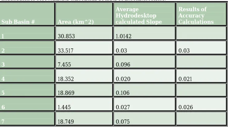
After the sub basins had been established. The area and slope of each sub basin were needed. Calculate the lag time and the time of concentration for each sub basin. The slope of each sub basin was measured and calculated by Hydrodesktop software. Due to the software being so new and the team’s lack of familiarity with the software, three sub basins were selected to have hand calculations performed to ensure the accuracy of the Hydrodesktop software. The results were extremely close, verifying the software’s accuracy. The results of the accuracy check can be seen in Table 2.1. The following table 2.1 displays the slopes calculated for each reach.The formula used to calculate slope is below.
TABLE B 2.1 DISPLAYS THE AREA OF EACH SUB BASIN AND THE AVERAGE SLOPES. SLOPE WAS PROVIDED BY HYDRODESKTOP SOFTWARE AND CALCULATED BY HAND TO ENSURE ACCURACY.
Sub Basin # Area (km^2)
Average
Hydrodesktop calculated Slope
Results of Accuracy Calculations
1 30.853 1.0142
2 33.517 0.03 0.03
3 7.455 0.096
4 18.352 0.020 0.021
5 18.869 0.106
6 1.445 0.027 0.026
7 18.749 0.075
S: Slope
21 | P a g e
t T: Lag Time
L: Hydraulic Length of the Watershed S: Watershed potential (=3.66)
Ws: Average slope of the Watershed
Tc = tL1.67 Tc=Time of Concentration (for individual sub
basin)
tL=Lag Time
2. Lag Time and Time of Concentration- 2.2
The average slope was needed to calculate the lag time. The equation below were used to calculate lag time for over land flow of each sub basin.
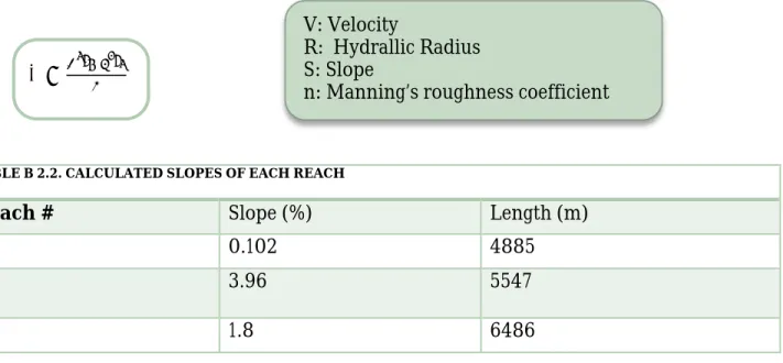
The time for each reach also had to be calculated. A version of Manning’s equation was used to solve for the velocity. The Velocity equation was then arranged to solve for time. The velocity was then used to find time using the velocity equaiton The input slope values for Manning’s equation can be found I Table B.2.2 below. Mannings’s equations was arranged as follows:
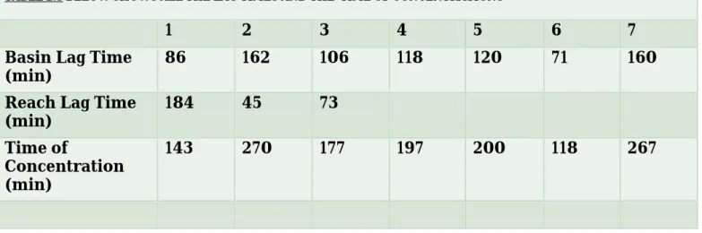
Lag time was used to calculate the time of concentration. The equation below was used to determine the time of concentration. Table 2.3 shows the lag times and time of concentration for all sub basins and reaches equation.
TABLE B 2.2. CALCULATED SLOPES OF EACH REACH
Reach # Slope (%) Length (m)
1 0.102 4885
2 3.96 5547
3 1.8 6486
V: Velocity
R: Hydrallic Radius S: Slope
22 | P a g e
Q= flow (cms) V=velocity (m^2/s) A=Area m^2
TABLE 2.3 BELOW SHOWS ALL THE LAG TIMES AND THE TIME OF CONCENTRATIONS
1 2 3 4 5 6 7
Basin Lag Time
(min) 86 162 106 118 120 71 160
Reach Lag Time (min)
184 45 73
Time of
Concentration (min)
143 270 177 197 200 118 267
3. Flow (Q) Calculations
A total flow (Q), at the point of concentration, was needed as an input parameter in Hec-HMS. The flow was calculated using the continuity equation. The velocity was calculated using
Manning’s equation. The velocity calculated at the end of reach three was used towards the final flow computations.
***Note Input values for equations and equation calculations are also found in Appendix B Q=VA
23 | P a g e
IX.
HEC-HMS 3.5
A.
Overview
This Hydrologic Modeling System (HEC-HMS) is designed to simulate the precipitation-runoff processes of dendritic watershed systems. It is designed to be applicable in a wide range of geographic areas for solving the widest possible range of problems. This includes large river basin water supply and flood hydrology, and small urban or natural watershed runoff.
Hydrographs produced by the program are used directly or in conjunction with other software for studies of water availability, urban drainage, flow forecasting, future urbanization impact, reservoir spillway design, flood damage reduction, floodplain regulation, and systems
operation. The program is a generalized modeling system capable of representing many different watersheds. A model of the watershed is constructed by separating the hydrologic cycle into manageable pieces and constructing boundaries around the watershed of interest. Any mass or energy flux in the cycle can then be represented with a mathematical model. In most cases, several model choices are available for representing each flux. Each mathematical model included in the program is suitable in different environments and under different conditions. Making the correct choice requires knowledge of the watershed, the goals of the hydrologic study, and engineering judgment. The program features a completely integrated work environment including a database, data entry utilities, computation engine, and results reporting tools. A graphical user interface allows the seamless movement between the different parts of the program. Program functionality and appearance are the same across all supported platforms.
1. Watershed Physical Description
The physical representation of a watershed is accomplished with a basin model. Hydrologic elements are connected in a dendritic network to simulate runoff processes. Available elements are: sub basin, reach, junction, reservoir, diversion, source, and sink. Computation proceeds from upstream elements in a downstream direction.
An assortment of different methods is available to simulate infiltration losses. Options for event modeling include initial constant, SCS curve number, gridded SCS curve number, exponential, and Green Ampt. The one-layer deficit constant method can be used for simple continuous modeling. The five-layer soil moisture accounting method can be used for
continuous modeling of complex infiltration and evapotranspiration environments. Gridded methods are available for both the deficit constant and soil moisture accounting methods.
24 | P a g e
Several methods are included for transforming excess precipitation into surface runoff. Unit hydrograph methods include the Clark, Snyder, and SCS techniques. User-specified unit hydrograph or s-graph ordinates can also be used. The modified Clark method, ModClark, is a linear quasi-distributed unit hydrograph method that can be used with gridded meteorologic data. An implementation of the kinematic wave method with multiple planes and channels is also included.
Multiple methods are included for representing base flow contributions to sub basin outflow. The recession method gives an exponentially decreasing base flow from a single event or multiple sequential events. The constant monthly method can work well for continuous simulation. The linear reservoir method conserves mass by routing infiltrated precipitation to the channel.
A variety of hydrologic routing methods are included for simulating flow in open channels. Routing with no attenuation can be modeled with the lag method. The traditional Muskingum method is included along with the straddle stagger method for simple approximations of attenuation. The modified Puls method can be used to model a reach as a series of cascading, level pools with a user-specified storage-discharge relationship. Channels with trapezoidal, rectangular, triangular, or circular cross sections can be modeled with the kinematic wave or Muskingum-Cunge methods. Channels with overbank areas can be modeled with the
Muskingum-Cunge method and an eight-point cross section.
Water impoundments can also be represented. Lakes are usually described by a user-entered storage-discharge relationship. Reservoirs can be simulated by describing the physical spillway and outlet structures. Pumps can also be included as necessary to simulate interior flood area. Control of the pumps can be linked to water depth in the collection pond and, optionally, the stage in the main channel.
2.
Meteorology DescriptionMeteorological data analysis is performed by the meteorologic model and includes precipitation, evapotranspiration, and snowmelt. Six different historical and synthetic
precipitation methods are included. Two evapotranspiration methods are included at this time. Currently, only one snowmelt method is available.
Four different methods for analyzing historical precipitation are included. The user-specified hyetograph method is for precipitation data analyzed outside the program. The gage weights method uses an unlimited number of recording and non-recording gages. The Thiessen technique is one possibility for determining the weights. The inverse distance method
25 | P a g e
can be used to automatically proceed when missing data is encountered. The gridded precipitation method uses radar rainfall data.
Four different methods for producing synthetic precipitation are included. The frequency storm method uses statistical data to produce balanced storms with a specific excedance probability. Sources of supporting statistical data include Technical Paper 40and NOAA Atlas 2. While it was not specifically designed to do so, data can also be used from NOAA Atlas 14. The standard project storm method implements the regulations for precipitation when estimating the standard project flood. The SCS hypothetical storm method implements the primary precipitation distributions for design analysis using Natural Resources Conservation Service (NRCS) criteria. The user-specified hyetograph method can be used with a synthetic hyetograph resulting from analysis outside the program.
Potential evapotranspiration can be computed using monthly average values. There is also an implementation of the Priestley-Taylor method that includes a crop coefficient. A gridded version of the Priestley-Taylor method is also available.
Snowmelt can be included for tracking the accumulation and melt of a snowpack. A
temperature index method is used that dynamically computes the melt rate based on current atmospheric conditions and past conditions in the snowpack.
3. Hydrologic Simulation
The time span of a simulation is controlled by control specifications. Control specifications include a starting date and time, ending date and time, and a time interval.
A simulation run is created by combining a basin model, meteorologic model, and control specifications. Run options include a precipitation or flow ratio, capability to save all basin state information at a point in time, and ability to begin a simulation run from previously saved state information.
Simulation results can be viewed from the basin map. Global and element summary tables include information on peak flow and total volume. A time-series table and graph are available for elements. Results from multiple elements and multiple simulation runs can also be viewed. All graphs and tables can be printed.
26 | P a g e
4. Parameter Estimation
Most parameters for methods included in subbasin and reach elements discharge must be available for at least one element before optimization can begin. Parameters at any element upstream of the observed flow location can be estimated. Six different objective functions are available to estimate the goodness-of-fit between the computed results and observed discharge. Two different search methods can be used to minimize the objective function. Constraints can be imposed to restrict the parameter space of the search method.
5. Analyzing Simulations
Analysis tools are designed to work with simulation runs to provide the depth-area analysis tool. It works with simulation runs that have a meteorologic model using the frequency storm method. Given a selection of elements, the tool automatically adjusts the storm area and generates peak flows represented by the correct storm areas.
6. GIS Connection
The power and speed of the program make it possible to represent watersheds with hundreds of hydrologic elements. Traditionally, these elements would be identified by inspecting a
topographic map and manually identifying drainage boundaries. While this method is effective, it is prohibitively time consuming when the watershed will be represented with many elements. A geographic information system (GIS) can use elevation data and geometric algorithms to perform the same task much more quickly. A GIS companion product has been developed to aid in the creation of basin models for such projects. It is called the Geospatial Hydrologic Modeling Extension (HEC-GeoHMS) and can be used to create basin and meteorologic models for use with the program.
7. Basin Models
Basin models are one of the main components in a project. Their principle purpose is to convert atmospheric conditions into streamflow at specific locations in the watershed. Hydrologic elements are used to break the watershed into manageable pieces. They are connected together in a dendritic network to form a representation of the stream system. Background maps can be used to aid in placing the elements in a spatial context.
27 | P a g e
8. Subbasin Elements
A subbasin is an element that usually has no inflow and only one outflow. It is one of only two ways to produce flow in the basin model. Outflow is computed from meteorologic data by subtracting losses, transforming excess precipitation, and adding baseflow. Optionally the user can choose to include a canopy component to represent interception and evapotranspiration. It is also optional to include a surface component to represent water caught in surface
depressional storage. The subbasin can be used to model a wide range of catchment sizes.
9. Hydrological Elements
The physical watershed is represented in the basin model. Hydrologic elements are added and connected to one another to model the real-world flow of the water in a natural watershed. A description of each hydrological element is given below in Figure 9.1 is a screenshot of Table 10 of the HEC-HMS 3.5 User Manual.
28 | P a g e
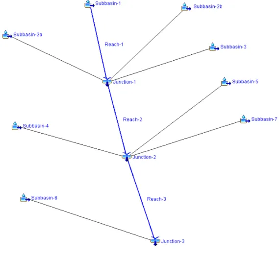
10. Project Watershed Model
Figure 10.1 below represents our modeled watershed. There are 8 different subbasins, 3 reaches, and 3 junctions. Since water cannot flow downstream through the soil, reaches are used. Junctions connect the subbasins and reaches and junction 3 is the point of concentration.
29 | P a g e
11. Precipitation Method
For our model we used a precipitation frequency of a frequency storm. The storm duration used for the study was a 24 hour event. This storm duration selected allows for all portions of the basins to contribute to the basin outlet and is based on the longest time of concentration in the model. The frequency data was found using NOAA for data found in Flagstaff. We took the frequency data for a 5 year, 10 year, 25 year, 50 year, and 100 year storm, and modelled all cases. Table B.11.1 below shows the data used in the modeling analyses. Figure 11.1 is a screen shot from NOAH
TABLE B 11.1 – DATA USED IN MODELING ANANLYSES Sub-basin Area
(sq km)
5 yr (cms)
10 yr (cms)
25 yr (cms)
50 yr (cms)
100 yr (cms)
1 30.85 65.1 84.2 113.5 138.4 166.4
2a 26.0 35.4 45.2 60.2 72.7 86.8
2b 7.52 10.2 13.1 17.4 21.0 25.0
3 7.46 13.7 17.7 23.7 28.8 34.5
4 18.35 31.3 40.2 53.8 65.3 78.2
5 18.87 31.8 40.8 54.7 66.3 79.4
6 1.45 3.5 4.5 6.1 7.4 8.9
30 | P a g e
12. Selecting a Loss Method
While a subbasin element conceptually represents infiltration, surface runoff, and subsurface processes interacting together, the actual infiltration calculations are performed by a loss method contained within the subbasin. A total of twelve different loss methods are provided. Some of the methods are designed primarily for simulating events while others are intended for continuous simulation. All of the methods conserve mass. That is, the sum of infiltration and precipitation left on the surface will always be equal to total incoming precipitation.
31 | P a g e
For our project modeling, two loss methods were used. These were the SCS Curve Number loss method, and the Green and Ampt loss method. Using two different loss methods, which take different input variables, gave us sensitivity analysis while running our model by getting output discharge values which were close but not the same exact values.
13. Selecting a Routing and Transform Method
For the routing method we stuck to using lag. Only using lag is a conservative approach
because doing so does not assume an attenuation of the hydrograph. For the transform method we used the SCS Unit Hydrograph method. This transform method was used for all pre-burn and post-burn conditions modelled. This transform method requires the lag times for both the subbasins and the reaches. The lag times for the subbasins were calculated by using the SCS Lag Time Equation, while the lag times for the reaches were found applying Manning’s
Equation. All equations used, equation input values, and results can be found in Section V.C.8 of this report.
14. SCS Curve Number Loss
The Soil Conservation Service (SCS) Curve Number (CN) model estimates precipitation excess as a function of cumulative precipitation, soil cover, land use, and antecedent moisture. Using the CN, a maximum retention can be found which is inputted into the model when calculating the lag times.
15. Green and Ampt Loss
The Green and Ampt infiltration method is essentially a simplification of the comprehensive Richard's equation for unsteady water flow in soil. The Green and Ampt method assumes the soil is initially at uniform moisture content, and infiltration takes place with so-called piston displacement. The method automatically accounts for ponding on the surface. The initial water content gives the initial saturation of the soil at the beginning of a simulation. It should be specified in terms of volume ratio. The saturated water content specifies the maximum water holding capacity in terms of volume ratio. It is often assumed to be the total porosity of the soil. The wetting front suction must be specified. It is generally assumed to be a function of the soil texture. The hydraulic conductivity must also be specified. It can be estimated from field tests or approximated by knowing the soil texture. The percentage of the subbasin which is directly connected impervious area can be specified. No loss calculations are carried out on the
32 | P a g e
impervious area; all precipitation on that portion of the subbasin becomes excess precipitation and subject to direct runoff.
16. Soil Classification and Input Variables
Using the Natural Resources Conservation Service’s Soil Conservation Maps Web Soil Survey, the soil in our watershed was classified as clay and was a Hydrological Soil Group D. This soil has a high potential for runoff with low infiltration, which allowed for conservative input values for our model. For our pre-burn modeling analysis, a curve number of 79 was used. We got this value from Appendix A of the HEC-HMS 3.5 Technical Reference Manual as it related to fair condition woods. Figure B 16.1 is a screen shot form Hec-HMS for curve numbers
33 | P a g e
For our immediate low post-burn modeling analysis a CN of 85 was used, and for our
immediate high post-burn modeling analysis a CN of 95 was used. These values were found to be fitting from “SUMMARY HYDROLOGIC MODELING REPORT Shultz Fire Drainage Master Plan” report.
For the Green and Ampt parameter input variables, Figure B. 16.2 is a screenshot of Table 12 from the Technical Reference Manual was used in correlation with the NRCS soil classification of clay loam.
X.
Results
A.
Pre-Burn
Discharge results were found for both pre-burn and post-burn analysis of the watershed. Results for both the SCS Curve Number method and for the Green and Ampt method for the pre-burn ended up being close to each other which proved the modelling to be accurate. Immediate high burn and low burn results were found and with analyzing these results it is evident that if a fire were to occur on our watershed, flooding would occur and flood right into
34 | P a g e
downtown Flagstaff. Tables R-1.1 and R1.2…. below show the pre-burn analysis results that were found when modelling both the SCS Curve Number loss method as well as the Green and Ampt loss method.
B.
Post Burn
After analyzing and modelling the pre-burn conditions or our watershed, we analyzed and modelled the immediate high post-burn conditions as well as the immediate low post-burn conditions. We did this by using the SCS Curve Number loss method. TablesR 1.3 andR 1.4 … below show the results found when modeling these conditions. For the immediate high post-burn conditions a CN of 95 was used, and for the immediate low post-post-burn condition a CN of 85 was used.
TABLE R1.1 PRE-BURN SCS CURVE NUMBER LOSS METHOD RESULTS
35 | P a g e
TABLE R1.4 IMMEDIATE LOW POST-BURN SCS CURVE NUMBER LOSS METHOD RESULTS TABLE R1.3 IMMEDIATE HIGH POST-BURN SCS CURVE NUMBER LOSS METHOD RESULTS
36 | P a g e Conclusion
After modelling the post-burn conditions of the watershed and looking at the results, it is evident that flooding would indeed occur. Table R1.4 below shows the outcomes from the different conditions evaluated within the model for the 100 year frequency data.
As you can see the discharges increased significantly when modeling the post-burn conditions. The two pre-burn loss method results were similar. TableR.1.5 below depicts interesting
comparison showing how the 10 year high post-burn modeling results are higher than the 100 year pre-burn modeling results.
37 | P a g e
This means that if a high burn high intensity fire were to occur on our watershed, then peak discharges would cause flooding into downtown Flagstaff. This is an important issue that needs to be addressed in order to prevent flooding. Methods include mechanical thinning of the Ponderosa Pines and mixed conifers in the area of study, as well as controlled burn fires. These methods would reduce fuel loading which in return would reduce the spread of fire, thus
reducing the flood rates which would occur when a storm hits Flagstaff. Many homes, county property, and even lives would be at danger. After modeling and analyzing the outcomes, precautionary measures should be taken to avoid drastic flooding of Flagstaff.
38 | P a g e
40 | P a g e
XII.
Appendix B
Sub-basin
Slope (%)
Length (m)
HSG Classification
1 14.2 10126 D CL
2 3.0 8472 D CL
3 9.65 10357 D CL
4 2.05 4490 D CL
5 10.41 12725 D CL
6 2.69 2792 D CL
7 7.57 14860 D CL
Reach
Slope (%)
Length (m)
1 0.102 4885
2 3.96 5547
41 | P a g e
Sub-basin
CN
Lag Time (min)
Tc (min)
1 85 71 118
2a 85 133 222
2b 85 133 222
3 85 87 145
4 85 97 162
5 85 99 165
6 85 58 97
7 85 132 220
Sub-basin
Lag Time (min)
Time of Concentration
(min)
1 86 143
2 162 270
3 106 177
4 118 197
5 120 200
6 71 118
42 | P a g e
Reach
Lag Time (min)
1 185
2 46
3 73
SCS Loss Curve Method
Sub-basin
Area (sq
km)
5 yr
(cms)
10 yr
(cms)
25 yr
(cms)
50 yr
(cms)
100 yr
(cms)
1 30.85 65.1 84.2 113.5 138.4 166.4
2a 26.0 35.4 45.2 60.2 72.7 86.8
2b 7.52 10.2 13.1 17.4 21.0 25.0
3 7.46 13.7 17.7 23.7 28.8 34.5
4 18.35 31.3 40.2 53.8 65.3 78.2
5 18.87 31.8 40.8 54.7 66.3 79.4
6 1.45 3.5 4.5 6.1 7.4 8.9
43 | P a g e
Green and Amp
Sub-basin
(sq km)
Area
(cms)
5 yr
(cms)
10 yr
(cms)
25 yr
(cms)
50 yr
100 yr
(cms)
1
30.85
66.4
90.2
124.7
153.6
185.5
2a
26.0
31.2
42.6
59.0
72.9
88.5
2b
7.52
9.0
12.3
17.0
21.0
25.5
3
7.46
13.2
18.0
25.0
30.8
37.2
4
18.35
29.6
40.3
55.9
68.9
83.5
5
18.87
29.9
40.8
56.5
69.6
84.4
6
1.45
3.7
5.0
6.9
8.5
10.2
44 | P a g e
Low Burn
Sub-basin
CN
Lag Time (min)
Tc (min)
1 85 71 118
2a 85 133 222
2b 85 133 222
3 85 87 145
4 85 97 162
5 85 99 165
6 85 58 97
7 85 132 220
High burn
Sub-basin
CN
Lag Time (min)
Tc (min)
1 95 47 78
2a 95 88 147
2b 95 88 147
3 95 58 97
4 95 64 107
5 95 65 108
6 95 38 63
45 | P a g e
Immediatie Post High Burn
Sub-basin
Area
(sq km)
5 yr
(cms)
10 yr
(cms)
25 yr
(cms)
50 yr
(cms)
100 yr
(cms)
1 30.85 159.2 195.2 247.9 291.8 339.2
2a 26.0 90.3 110.1 139.1 163.1 189.3
2b 7.52 26.0 31.8 40.1 47.0 54.6
3 7.46 33.9 41.6 52.8 62.1 72.1
4 18.35 78.7 96.3 122.1 143.4 166.7
5 18.87 80.2 98.2 124.4 146.1 169.8
6 1.45 8.5 10.5 13.3 15.7 18.2
46 | P a g e
Immediate Post Low Burn
Sub-basin Area (sq
km)
5 yr (cms) 10 yr
(cms)
25 yr (cms)
50 yr (cms)
100 yr (cms)
1 30.85 89.9 114.6 151.7 182.9 217.4
2a 26.0 49.5 62.3 81.5 97.5 115.3
2b 7.52 14.3 18.0 23.5 28.1 33.3
3 7.46 18.9 24.1 31.8 38.3 45.4
4 18.35 43.5 55.2 72.7 87.4 103.7
5 18.87 44.0 55.8 73.6 88.4 104.9
6 1.45 4.8 6.1 8.1 9.8 11.6
47 | P a g e
XIV.
Works Cited
There are no sources in the current document. US Topographic Maps
http://www.arcgis.com/home/webmap/viewer.html?webmap=931d892ac7a843d7ba29d085e 0433465
US Army Corps of Engineers Hydrologic Modeling System HEC-HMS Technical Reference Manual
http://websoilsurvey.sc.egov.usda.gov/App/HomePage.htm Coconino National Forest Terrestrial Ecosystem Survey
http://websoilsurvey.sc.egov.usda.gov/App/WebSoilSurvey.aspx http://www.tucson.ars.ag.gov/unit/publications/aspfiles/listing.asp Coconino County Drainage Design Manual
http://www.coconino.az.gov/DocumentCenter/View/1789
“Munds Park Risk MAP Study (Coconino County, AZ)” FEMA Case No. 12-09-1963S. http://www.cpesc.org/reference/tr55.pdf
http://www.fs.fed.us/rm/pubs_other/rmrs_2011_neary_d003.pdf For hydrologic impacts of high severity.
USGA National Map Data Seamless Server NOAA Precipitation Data Server
Coconino National Forest County Terrestrial Ecosystem Survey
48 | P a g e
USFS BEAR Road Treatment Tools – Curve Numbers Methods Supplement
USFS Shultz Fire Sub Basin Watershed and Severity Map, July, 2010
“Shultz Fire/Flood. The Disaster that Keeps Giving.” Archuleta, Liz. Metzger, Mandy. “SUMMARY HYDROLOGIC MODELING REPORT Shultz Fire Drainage Master Plan”
“FLOOD GYDROLOGY NEAR FLAGSTAFF, ARIZONA” Hill, G.W. Hales, T.A. Aldridge, B.N. Leao, Duncan, Water Yield and Peak Discharges Resulting From Forest Disturbances in a Northern
Arizona Watershed. Flagstaff: Northern Arizona University, 2005. Print.
Omi, P.N. and E.J. Martinson. 2002. Effects of fuels treatments on wildfire severity. Western Forest Fire Research Center, Colorado State University.
Rothermel, R. C.; Wilson, R. A.; Morris, G. A.; Sacket, S. S. 1986. Modeling moisture content of fine dead wildland fuels: input to the BEHAVE fire prediction system. Research Paper INT‐359. Ogden, UT: U.S. Department of Agriculture, Forest Service, Intermountain Forest and Range.
WAGENER, W. W. 1961. Guidelines for estimating the survival of fire‐damaged trees in California.
USDA For. Servo Misc. Pap. 60. 11 p.
WYANT, J. G., P. N. OMI, and R. D. LAVEN. 1986. Fire induced tree mortality in a Colorado ponderosa pine/Douglas‐fir stand. For. Sci. 32:49‐59.