BIROn - Birkbeck Institutional Research Online
Abakuks, Andris (2012) The synoptic problem: on Matthew’s and Luke’s use
of Mark. Journal of the Royal Statistical Society: Series A 175 (4), pp.
959-975. ISSN 0964-1998.
Downloaded from:
Usage Guidelines:
Please refer to usage guidelines at or alternatively
BIROn
-
B
irkbeck
I
nstitutional
R
esearch
On
line
Enabling open access to Birkbeck’s published research output
The synoptic problem: on Matthew's and Luke's use of
Mark
Journal Article
http://eprints.bbk.ac.uk/4262
Version: Accepted (Refereed)
Citation:
© 2011
Wiley Blackwell
Publisher site
______________________________________________________________
All articles available through Birkbeck ePrints are protected by intellectual property law, including copyright law. Any use made of the contents should comply with the relevant law.
______________________________________________________________
Deposit Guide
Contact: [email protected]
Birkbeck ePrints
Birkbeck ePrints
Abakuks, A. (2011)
The synoptic problem: on Matthew's and Luke's use of Mark –
The synoptic problem: on Matthew’s and Luke’s use
of Mark
Andris Abakuks
∗Birkbeck College, University of London, UK
October 2011
Summary. In New Testament studies, the synoptic problem is concerned with the rela-tionships between the gospels of Matthew, Mark and Luke. Assuming Markan priority, we investigate the relationship between the words in Mark that are retained unchanged by Matthew and those that are retained unchanged by Luke. This is done by mapping the sequence of words in Mark into binary time series that represent the retention or non-retention of the individual words, and then carrying out a variety of logistic regression analyses.
Keywords: New Testament; synoptic problem; Markan priority; binary time series;
vari-able length Markov chain; generalized linear model; logistic regression; generalized linear mixed model
1
Introduction
In New Testament studies the synoptic problem is concerned with hypotheses about
the relationships between the synoptic gospels of Mark (Mk), Matthew (Mt) and Luke (Lk). The Gospel of John is not included, as it is very different in style and in the detail of its content. In Abakuks (2006a, 2007) versions of the triple-link model in the
synoptic problem were examined, building on aspects of the statistical analysis of Honor´e
(1968). According to the triple-link model, Gospel A was written first, Gospel B was written second and used Gospel A as a source, and Gospel C was written third and used both Gospel A and Gospel B as sources, where A, B, C is any permutation of Mt, Mk, Lk. An outline of this work together with some background material is given in Abakuks (2006b), and good introductions to the synoptic problem more generally are provided by Goodacre (2001) and Kloppenborg (2008). A comprehensive survey of statistical approaches to the synoptic problem is provided by Poirier (2008). Although the triple-link model essentially includes as special cases a number of models that are currently being advocated to describe the relationships between the synoptic gospels, it does not include what is still the most commonly accepted model, the source or two-document hypothesis, according to which Matthew and Luke had two sources in common,
∗Address for correspondence: Department of Economics, Mathematics and Statistics, Birkbeck
Mark and a hypothetical “Q”, both of which Matthew and Luke used independently of each other. The present paper will be based upon the commonly accepted assumption of Markan priority, that is, that the gospel of Mark was the first to be written and that the authors of the gospels of Matthew and Luke used the text of Mark as a basis for their own gospels, but making alterations, omissions and additions. This assumption is implicit in the two source hypothesis, but does not imply it.
In considering the differences between the texts of the synoptic gospels, the role of oral tradition should also be borne in mind. It has long been accepted that in the early church oral traditions played an important role in the transmission of the material that came to be incorporated into the gospels. However, as pointed out by Dunn (2003a, 2003b), discussion of the synoptic problem has come to be in terms of literary relationships, while the role of oral transmission has faded into the background. Dunn has now attempted to reverse this tendency by emphasising the essentially oral culture in which the gospel writers operated. The transmission of gospel material would have been through oral performance, where the performers, or teachers, would faithfully transmit core material about the life and, perhaps especially, the teaching of Jesus, but where there would be considerable flexibility and variation from performance to performance in the details of the presentation. The gospel writers would have been immersed in a culture of such oral performance even if they also had some written sources available, and, as the gospels came to be written and started to circulate in document form, the primary means of transmission of Jesus traditions in what was predominantly a non-literate society would still have been through oral performance. Where there are considerable discrepancies among the texts of the synoptic gospels, this may be particularly suggestive of the influence of oral tradition. For further discussion of these ideas see also Bauckham (2006).
In the standard form of the two-source hypothesis, it is assumed that Matthew and Luke were independent in their use of Mark, in the sense of not collaborating or neither having the other’s text available as a source. Although this might suggest that they were statistically independent in the choice of the words that they retained from Mark, this is not necessarily the case. We might expect the criteria that Matthew and Luke used to select words from Mark to have some similarities. What they regarded as important to retain precisely word for word might have some common features, as might what they regarded as superfluous or problematical. Furthermore, they might both have been influenced by similar verbal traditions that affected their use of Mark in similar ways. The result would be that there would be some departures from statistical independence. As alternatives to the two-source hypothesis, we may consider the two cases of the triple-link model that assume Markan priority but dispense with the need for the “Q” source. Firstly, there is the Farrer hypothesis, according to which Matthew used Mark, but Luke used both Mark and Matthew. This has recently received considerable support, for example, in Goodacre (2002) and Goodacre and Perrin (2004). Secondly there is the possibility that Luke used Mark, but Matthew used both Mark and Luke. This has the support of Hengel (2000). Under either of these two models, we could expect there to be a much stronger statistical dependence between the words that Matthew and Luke retained from Mark than is the case with the two-source hypothesis. More specifically, we might look for evidence that the text of Matthew influenced Luke’s use of Mark or that the text of Luke influenced Matthew’s use of Mark.
be used, which at its heart consists of a bivariate binary time series that represents Matthew’s and Luke’s use of Mark. Before embarking on a more detailed examination of the dependency between Matthew’s and Luke’s use of Mark, in Section 3 we attempt to model the way in which Matthew and Luke each individually used the text of Mark. After an exploratory analysis based upon the fitting of variable length Markov chains, logistic regression models are fitted to the binary time series. In Section 4 we introduce terms into the logistic regression models that allow for the influence of Luke on Matthew’s use of Mark and vice-versa. Even after allowance is made for other factors, there still remains very strong evidence of dependency. In Section 5, some pointers are provided to further statistical work that could be done to investigate the relationships between the synoptic gospels.
2
The data
As in the earlier work of Abakuks (2006a, 2007), the statistical analysis here will be based upon observation of verbal agreements between the synoptic gospels, that is, of common occurrences of the same Greek word in the same context and in the same grammatical form. In the earlier work, as emphasized in Abakuks (2007), the results of the analysis of the triple-link model were presented with no formal indication of their statistical signifi-cance. A major problem in attempting to develop any statistical methodology is that the individual words in the text cannot even remotely be regarded as behaving independently of each other. Words tend to be transmitted unaltered from one gospel to another in clus-ters of varying sizes, and there are large segments of material that are not transmitted at all. (A notable example is Luke’s “great omission”, where he appears to have made no use of the section of Mark’s text from Mk 6:45 - 8:10.) Because of this, there is no simple way of writing down a likelihood function corresponding to the triple-link model and then using standard methods for statistical inference.
A new feature of the present paper is that in constructing a data set for analysis and then in developing a statistical model we are explicitly going to take into account the word
order in Mark. Farmer in his Synopticon (1969) presented the Greek text of each of the
synoptic gospels and highlighted individual words in different colours to indicate which of them appeared in the same context and in exactly the same grammatical form in each of the other two synoptic gospels. In the case of Mark’s gospel, words that appear unchanged in Matthew only are highlighted in yellow, words that appear unchanged in Luke only are highlighted in green, and words that appear unchanged in both Matthew and Luke are highlighted in blue. For most sections of Mark’s text, it is quite clear which are the parallel sections of text in Matthew and Luke and then it is generally straightforward to observe, assuming Markan priority, which words have been retained unchanged by Matthew and Luke, although even here there may be occasional differences of opinion. Elsewhere, for example, where Matthew or Luke have reordered sections of Mark’s text, and especially where there are doublets, two apparently alternative versions of the same section of Mark’s text, in Matthew or Luke, it may be a matter of judgement which, if any, sections of Matthew or Luke to regard as parallel to a given section of text in Mark. Here there may be substantial differences of opinion as to which words in Mark have been retained unchanged by Matthew or Luke. A helpful overview of where different sections of
Relationships (1995). Another issue is that different authors may be using different critical editions of the Greek text, although the differences here are minor. Farmer used the 25th edition of the standard Nestle-Aland text, Nestle and Aland (1963), whereas the current
edition is the 27th. In the present paper we shall use data based upon Farmer’sSynopticon
and consequently follow his evaluations of verbal agreements. The experience in Abakuks (2007) of comparing the results of the analysis of the triple-link model using two different
data sets of verbal agreements, those of Honor´e (1968) and Tyson and Longstaff (1978),
suggests that, if an alternative evaluation of verbal agreements were used, the overall conclusions here too would not be seriously affected.
The data set that we shall use is a word by word transcription of Farmer’s colour-coded text into a bivariate binary time series of length 11078, which is the number of words in the Greek text of Mark that was used by Farmer (but finishing at Mk 16:8 and excluding the longer ending, which is generally regarded as a later addition to the text). Verbal
agreements are coded 1 and non-agreements 0. The first component (xt) of the bivariate
time series is constructed by writing 1 if a word is present unchanged in Matthew and
0 otherwise. The second component (yt) is constructed by writing 1 if a word is present
unchanged in Luke and 0 otherwise. The subscript of the time series refers to the position of the word in the text of Mark. It should be noted that the data could be regarded as a spatial process in one dimension, but in fact there is a natural direction to the data, the order in which the text was written down by Mark and in which it was read by Matthew and Luke, so that it is more natural to think of the data as a time series, which is what is done in the present approach.
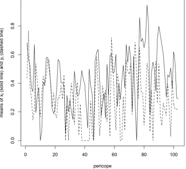
[image:6.595.188.411.496.630.2]The total numbers of zeros and ones represent counts of verbal agreements and non-agreements between Mark and the other synoptic gospels. These counts are presented in Table 1 in the form of a contingency table, which enables us to make some simple initial observations. By inspection of the row and column totals we see that overall Matthew
Table 1: Counts of verbal agreements with Mark
Luke
0 1 total
0 5243 1119 6362
(4606) (1756)
Matthew
1 2778 1938 4716
(3415) (1301)
total 8021 3057 11078
independence. Because, as pointed out earlier, the individual words in Mark cannot be regarded as a random sample, the simple chi-square tests of association will not be valid. Nevertheless, it is worth noting that if we mechanically carry out a simple chi-square test then we obtain a chi-square value of 749 on 1 degree of freedom, with a correspondingly miniscule p-value. This does at least suggest that there may be serious evidence that Matthew and Luke are not statistically independent in their verbal agreements with Mark, and our time series analysis will confirm this.
One way in which a statistical dependency between Matthew’s and Luke’s use of Mark, might have arisen, even if they were working independently of each other, is if they used similar criteria in deciding what types of text it was important to retain unchanged. Mor-genthaler (1971) in his major statistical analysis of the texts of the gospels distinguished between several types of text. Tyson and Longstaff (1978) too classified sections of text as to whether they were narrative material or words of Jesus or John the Baptist, i.e., material that is often referred to as “sayings”.
From the Greek text of the Gospel of Mark it is easy to specify precisely which words make up the direct speech of Jesus. There is also a short piece of the direct speech of John the Baptist and two short pieces of direct speech representing the divine voice from
heaven. We have constructed another binary time series (zt), where at any point the value
1 represents a word that is part of the direct speech of Jesus or John or the divine voice and 0 represents a word which is not part of such direct speech. Biblical scholars generally agree that the writers of the gospels and those who transmitted the tradition orally through public performance would have had a greater tendency to reproduce precisely word for word the sayings of Jesus or John but would have felt more at liberty to vary the narrative and editorial material and the speech of other participants in the narrative.
Hence it seems appropriate to introduce zt as a covariate into our models to investigate
the extent to which it helps to explain the variation in the series (xt) and (yt) and the
dependence between them.
The texts of the gospels may be partitioned into sections, referred to as pericopes
by biblical scholars. Each such pericope is a reasonably self-contained section of text, as discussed briefly in Abakuks (2006b). Different authors may differ in the details of the specification of the pericopes, but on the whole there seems to be broad agreement about the structure of most of the pericopes. Two standard specifications are provided by Huck (1949) and Aland (1996), respectively. We shall make use of the former, which is geared specifically to comparison of the three synoptic gospels and which partitions the Gospel of Mark into 103 pericopes that range in length from 15 to 374 words. To take into account that there may be variation in the way that Matthew and Luke handle the different Markan pericopes, we shall introduce a factor for pericope into our models.
For the present, to illustrate in outline the way in which the series (xt) and (yt) vary
over the length of Mark’s gospel, in Figure 1 we provide a plot of the mean values of xt
(the solid line) and yt (the dashed line) by pericope, where for the purposes of this plot
the pericopes have been numbered 1 to 103 in the order in which they appear in Mark’s gospel. These means are, equivalently, the proportions of Mark’s words that are retained unchanged by Matthew and Luke, respectively. As may be seen from the plots, there is a great deal of variation in these means among the pericopes. As observed in the comments
on Table 1, the overall mean for xt is 0.43 and for yt is 0.28, and this is reflected in the
pericope
0 20 40 60 80 100
0.0
0.2
0.4
0.6
0.8
means of
xt
(solid line) and
yt
[image:8.595.105.477.241.579.2](dashed line)
3
Models for the univariate series
In this section, as a preliminary, we shall consider the modelling of the time series (xt)
that represents the sequence of verbal agreements (denoted by 1) and non-agreements
(denoted by 0) of Matthew with Mark, and of the corresponding series (yt) for Luke,
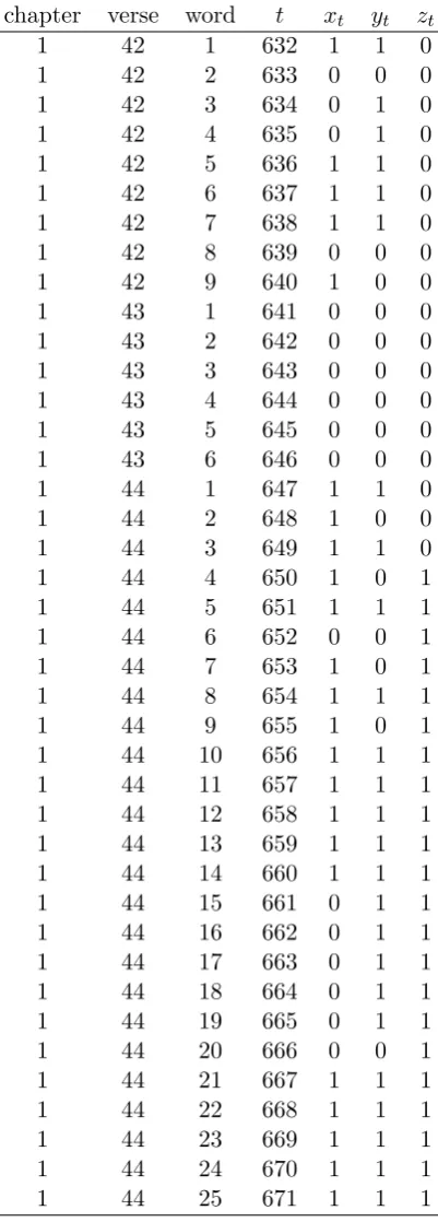
when the series are considered individually. For illustration, a section of the series is
shown in Table 7 in Appendix A, together with the covariate series (zt).
When either of the series (xt) and (yt) is examined, it becomes apparent that at any
point t the probability of a 1 occurrring depends on the previous history of the series. A
previous run of 0s makes it less likely that there will be 1 in the current position, but a previous run of 1s will make it more likely that there will be a 1 in the current position. In other words, there is some clustering of 1s and of 0s.
One approach to modelling categorical, and in particular binary, time series is by using variable length Markov chains (VLMCs). This method is described, for example,
by M¨achler and B¨uhlmann (2004), who also introduce the R package VLMC that provides
an algorithm for fitting VLMCs. In a VLMC model the order of the Markov chain that is used at any point depends on the history of the process, i.e., the transition probabilities are determined by looking back at a variable number of lagged values of the series. The numbers of lags used in a particular fitted model will depend upon the tuning parameters chosen for the VLMC algorithm.
When the results of applying the VLMC algorithm in R to the series (xt) and (yt)
were examined, no particularly illuminating models emerged nor was there any clear-cut indication of the number of lags that should be used. What did emerge, however, was that the transition probabilities generated by the models suggested by the VLMC algorithm were based upon the number of 0s since the last occurrence of 1 and, to a lesser extent, the number of 1s since the last occurrence of a 0.
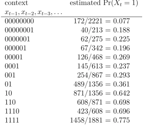
Table 2 shows a VLMC model fitted to the series (xt). In this case the overall order of
the fitted Markov chain is 8, the maximum number of lagged values of the series used in
the fitted model. The termcontext here refers to the relevant historyxt−1, xt−2, xt−3, . . .of
the process at any point t, and the estimated probability, given any particular context, is
simply the relative frequency in the observed run of the series of the occurrence of xt= 1
over all occurrences of the given context.
So, viewing the VLMC algorithm as an exploratory technique, what was suggested was that useful predictors of the next value in the series might be the current run lengths of 0s and 1s, or some function of them, and that these would provide a compact way of representing the effect of the history of the process upon the probability distribution of the next value, perhaps to a large extent replacing what might otherwise be a complicated function of several lagged values and their interactions.
For the main part of our analysis, we use generalized linear modelling, which in a time series setting is presented in Kedem and Fokianos (2002), where the use of the standard methods of generalized linear modelling, as provided by McCullagh and Nelder (1989), is justified for the analysis of time series through a partial likelihood approach. Kedem and Fokianos (2002) in their Chapter 2 deal specifically with the case of binary time series, including the use of logistic regression.
Assuming that the series has been observed up to the (t−1)th position, or, equivalently,
in the language of time series, assuming that the process has been observed up to time
Table 2: A fitted VLMC model for the series (xt)
context estimated Pr(Xt = 1)
xt−1, xt−2, xt−3, . . .
00000000 172/2221 = 0.077
00000001 40/213 = 0.188
0000001 62/275 = 0.225
000001 67/342 = 0.196
00001 126/468 = 0.269
0001 145/613 = 0.237
001 254/867 = 0.293
01 489/1356 = 0.361
10 871/1356 = 0.642
110 608/871 = 0.698
1110 423/608 = 0.696
1111 1458/1881 = 0.775
series (xt),
πt= Pr(Xt = 1|Ft−1),
where the upper case Xt represents the binary random variable at time t and Ft−1 the
history of the process up to time t−1.
Let Nt0 denote the current run of 0s at time t and Nt1 denote the current run of 1s,
where one or other of N0
t and Nt1 will always be zero. From the exploratory analysis
using VLMCs, it was found that N0
t−1 and Nt1−1 might be especially important predictor
variables forπt. In fact, some further investigation showed that better predictor variables,
as judged by comparison of the residual deviances of the fitted models, were given by
taking logarithms and using R0
t−1 and Rt1−1, where
R0t = ln(1 +Nt0)
and
R1t = ln(1 +Nt1) .
It was also anticipated that, in addition, the recent history of the process might be
partic-ularly influential so that, to supplement the information in the variables R0
t−1 and R1t−1,
a small number of the lagged variables Xt−1, Xt−2, . . . might also be used as predictors,
and possibly their interactions. Using other link functions in the generalized linear model appeared to do no better than using the canonical logit link, so the model adopted was of the form
ln
πt
1−πt
=α+β0Rt0−1+β1R1t−1 +γ1Xt−1 +γ2Xt−2, (1)
but envisaging the possibility that not all the terms would be needed or that some further lagged terms and interactions might be added.
Similarly, if θt is the probability that there is a 1 in position t for the series (yt), the
model adopted was of the form
ln
θt
1−θt
[image:10.595.184.415.110.315.2]
where S0
t and St1 are the logarithms of the run lengths defined in exactly the same way
as R0
t and R1t for the series (xt).
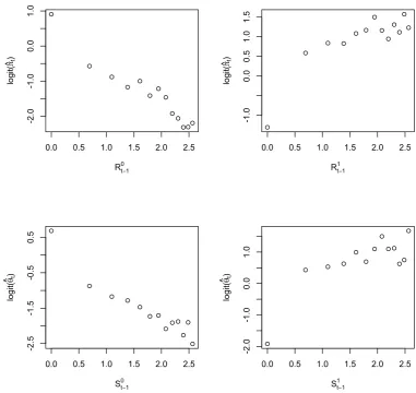
As a check on the appropriateness of regressing the logits on the logarithms of run
lengths for the series (xt), simple estimates ˆπt of Pr(Xt = 1) were calculated conditional
upon the values of the run lengthsN0
t−1 andNt1−1, using as estimates the values of relative
frequencies, just as in Table 2 for the VLMC model. In Figure 2 the logits of ˆπt have
been plotted against values of R0
t−1 and Rt1−1. Using a similar calculation for the series
(yt), the logits of ˆθt have been plotted against values of St0−1 and St1−1. The plots appear
to be reasonably linear except for the zero values of the regressor variable, but these are
special values because, for example, when one of R0
t−1 and R1t−1 is zero and absent from
the regression then the other is non-zero and contributes to the regression. Furthermore,
the possible presence of the regressor variables Xt−1, Xt−2, . . . and interaction terms may
effect a further adjustment to the regression if this turns out to be necessary.
0.0 0.5 1.0 1.5 2.0 2.5
-2.0
-1.0
0.0
1.0
Rt−10
logit(
π
^)t
0.0 0.5 1.0 1.5 2.0 2.5
-1.0
0.0
0.5
1.0
1.5
Rt1−1
logit(
π
^)t
0.0 0.5 1.0 1.5 2.0 2.5
-2.5
-1.5
-0.5
0.5
St0−1
logit(
θ
^)t
0.0 0.5 1.0 1.5 2.0 2.5
-2.0
-1.0
0.0
1.0
St−11
logit(
θ
[image:11.595.97.479.305.665.2]^)t
Figure 2: Plots of logits against logarithms of run lengths
Models of the form of Equation (1) and Equation (2) were fitted to the series (xt)
function was used for stepwise selection of predictor variables starting from the null model,
where in practice the method led to forward selection of variables. The step function
is based upon the use of the Akaike information criterion (AIC), but it also outputs the values of residual deviance at each step, which enables tests of significance to be carried out, based on the asymptotic likelihood ratio test.
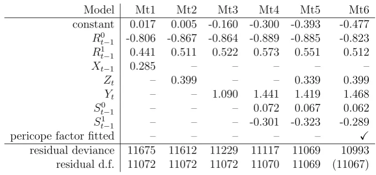
When a model of the form of Equation (1) were fitted to the series (xt) that represents
Matthew’s use of Mark, it was found that the best single predictor to use was R0
t−1. A
highly significant improvement in fit was obtained by including also R1
t−1 as a predictor.
A further significant improvement was obtained by includingXt−1, but then no significant
[image:12.595.103.491.349.530.2]improvement was obtained by introducing further lagged variables. It should be recalled that for binary data it is not appropriate to use the residual deviance as an absolute measure of the goodness of fit of the model. See Kedem and Fokianos (2002), p. 66, and McCullagh and Nelder (1989), pp. 121-122. So the question of how well the model fits the data is left somewhat open, although it is appropriate to look at changes in residual deviance when assessing the significance of introducing additional terms into the model. The estimated regression coefficients for this model (Mt1) are given in Table 3.
Table 3: Estimated regression coefficients for the series (xt)
Model Mt1 Mt2 Mt3 Mt4 Mt5 Mt6
constant 0.017 0.005 -0.160 -0.300 -0.393 -0.477
R0t−1 -0.806 -0.867 -0.864 -0.889 -0.885 -0.823
R1
t−1 0.441 0.511 0.522 0.573 0.551 0.512
Xt−1 0.285 – – – – –
Zt – 0.399 – – 0.339 0.399
Yt – – 1.090 1.441 1.419 1.468
S0
t−1 – – – 0.072 0.067 0.062
St1−1 – – – -0.301 -0.323 -0.289
pericope factor fitted – – – – – X
residual deviance 11675 11612 11229 11117 11069 10993
residual d.f. 11072 11072 11072 11070 11069 (11067)
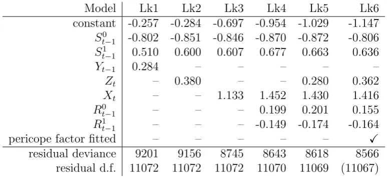
A similar fitted model (Lk1) of the form of Equation (2) emerges for the series (yt)
that represents Luke’s use of Mark. Its estimated regression coefficients are given in Table 4. In what follows, as further variables are introduced into the regression equations, each column in Tables 3 and 4 will represent the model chosen as a result of a stepwise procedure for the current set of candidate variables.
We next consider introducing the covariate series (zt) for direct speech and using Zt
as an additional predictor variable for the series (xt) and (yt). When modelling the series
(xt), we find again that the best pair of predictors to use is R0t−1 and Rt1−1, but the next
variable that provides the greatest improvement in fit is Zt. The estimated regression
coefficients for the resulting model (Mt2) are given in Table 3. Further significant but
small improvements in fit are given by introducing the interaction of Zt with R1t−1 and
then Xt−1 into the model. However, we have chosen to present the simpler model Mt2,
Table 4: Estimated regression coefficients for the series (yt)
Model Lk1 Lk2 Lk3 Lk4 Lk5 Lk6
constant -0.257 -0.284 -0.697 -0.954 -1.029 -1.147
S0
t−1 -0.802 -0.851 -0.846 -0.870 -0.872 -0.806
S1
t−1 0.510 0.600 0.607 0.677 0.663 0.636
Yt−1 0.284 – – – – –
Zt – 0.380 – – 0.280 0.362
Xt – – 1.133 1.452 1.430 1.416
R0t−1 – – – 0.199 0.201 0.155
R1
t−1 – – – -0.149 -0.174 -0.164
pericope factor fitted – – – – – X
residual deviance 9201 9156 8745 8643 8618 8566
residual d.f. 11072 11072 11072 11070 11069 (11067)
complex, and for ease of presentation and interpretation it was decided at this stage to keep to a simpler model. In so doing, nothing essential to the argument in Section 4 is lost.
Similarly, when modelling the series (yt), we find again that the best pair of predictors
to use is S0
t−1 and St1−1, but the next variable that provides the greatest improvement in
fit is Zt. The estimated regression coefficients for the resulting model (Lk2) are given in
Table 4. Further significant but small improvements in fit are given by introducing the
interaction of Zt with St0−1 and then Yt−1 into the model.
We see from the residual deviances that the covariate Zt for direct speech does give
some improvement in fit for the univariate series. Clearly, a word that is a part of direct speech is more likely to be retained unchanged by Matthew or Luke than a word that is a part of the narrative.
The remaining models, Mt3, . . . , Mt6 and Lk3, . . . , Lk6, in Tables 3 and 4,
respec-tively, include terms that model the dependency between the series (xt) and (yt) and will
be discussed in Section 4.
4
Models for the bivariate series
We now consider the two series (xt) and (yt) as a bivariate time series (xt, yt). In so doing
we are considering in conjunction Matthew’s and Luke’s use of Mark and their possible use of each other.
One type of approach that might naturally be considered here is the modelling of
the joint distribution of Xt and Yt in terms of the histories of the processes up to time
t−1. We could consider a bivariate logistic model as done in Sections 6.5.6 and 6.5.7 of
McCullagh and Nelder (1989) and as put in the more general setting of vector generalized
additive models by Yee and Wild (1996) and implemented in the R packageVGAM. Such an
approach is taken specifically for certain types of bivariate binary time series by Mosconi and Seri (2006), though using a probit rather than a logit link function.
is using Luke or Luke is using Matthew as a source, suggests that it is more natural to
model the distributions of Xt and Yt separately: Xt not only in terms of its own history
Ft−1 up to time t−1 but also in terms of the history Gt of the process (Yt) up to time
t, including, importantly, the current value Yt; and, similarly, Yt not only in terms of
its own history Gt−1 up to time t−1 but also in terms of the history Ft of the process
(Xt) up to timet, including the current value Xt. Furthermore, it may be illuminating to
consider our analysis in relation to the concept of causality as discussed in the econometric literature, where causality is expressed in terms of prediction. In particular, using the
terminology of Granger (1969), there is instantaneous causality of (Yt) acting on (Xt)
if the current value of Xt is better predicted when the current value Yt is included as
a predictor variable than when it is not. It should be noted, though, that even if it is found that there is causality in this specific sense, this will not establish that Luke is a
source for Matthew, although it may lend support to such a hypothesis. Similarly, if Yt
is better predicted when the current valueXt is included as a predictor variable, this will
not establish that Matthew is a source for Luke.
Adopting this approach, when modelling the series (xt) that represents Matthew’s use
of Mark, we consider as predictor variables not only the variables used in Section 3 that
are functions ofFt−1 but also the corresponding variables that are functions ofGt−1 and,
additionally, the current value Yt. For the present, we do not use the covariate Zt. When
variables were entered stepwise into the model equation, it was found, as in Section 3,
that the best single predictor to use wasR0
t−1, but the next best variable to enter was Yt,
and only at the third step did the variableR1t−1 enter into the equation. All three of these
variables provided a highly significant contribution to the fit. The estimated regression coefficients for the resulting model, Mt3, are given in Table 3. Comparison of the residual deviances shows that model Mt3 gives a substantial improvement in fit over the model Mt1, and like model Mt1 it has a simple natural interpretation: the probability of a word in Mark being used unchanged by Matthew decreases as the length of a previous run of non-usage increases and increases as the length of a previous run of usage increases, and also increases if the word is used unchanged by Luke. Further highly significant
improvements in fit are found by bringing in further variables from the process (Yt) to
obtain a model Mt4, whose estimated regression coefficients are given in Table 3, whereas
bringing in the variable Xt−1 gives only a relatively small improvement in fit. However,
the signs of the estimated regression coefficients for the additional terms S0
t−1 and St1−1 in
the model Mt4 are rather puzzling.
A very similar scenario emerged when models were fitted to the series (yt) that
rep-resents Luke’s use of Mark, considering the same predictor variables as before that are
functions of Gt−1 and Ft−1 and, additionally, the current value Xt. When variables were
entered stepwise into the model equation, it was found, as in Section 3, that the best
single predictor to use was S0
t−1, but the next best variable to enter was Xt, and only at
the third step did the variable St1−1 enter into the equation. All three of these variables
provided a highly significant contribution to the fit. The estimated regression coefficients for the resulting model, Lk3, are given in Table 4. Comparison of the residual deviances shows that model Lk3 gives a substantial improvement in fit over the model Lk1. Further highly significant improvements in fit are found by bringing in further variables from the
process (Xt) to obtain a model Lk4, whose estimated regression coefficients are given in
Table 4, whereas bringing in the variable Yt−1 gives only a relatively small improvement
additional termsR0
t−1 andRt1−1 in the model Lk4 are not what might have been expected.
An important question concerns the extent to which the introduction of the covariate
Ztfor direct speech into the models Mt4 and Lk4 will be able to account for the statistical
dependence between whether a word is retained unchanged by Matthew and whether it
is retained unchanged by Luke. We now consider the series (xt) and (yt) using the same
predictor variables as in the models Mt4 and Lk4 but with the addition of the variableZt.
When modelling the series (xt) using a stepwise approach, we find again that the predictor
variables enter into the model equation in the order R0
t−1,Yt,R1t−1, withZt entering only
at step 5. The model Mt4 with the addition of Ztas a predictor variable gives the model
Mt5 with estimated regression coefficients as given in Table 3. The introduction of the
variable Zt does give a significant improvement in fit but has very little impact on the
conclusion that the probability that a word is retained unchanged by Matthew is strongly dependent upon whether it is retained unchanged by Luke. Similarly, when modelling
the series (yt) using a stepwise approach, we find again that the predictor variables enter
into the model equation in the order St0−1, Xt, St1−1, with Zt entering only at step 5.
The model Lk4 with the addition of Zt as a predictor variable gives the Model Lk5 with
estimated regression coefficients as given in Table 4. Just as when modelling the series for Matthew, so when modelling the series for Luke, we find that the introduction of the
variable Zt has very little impact on the conclusion that the probability that a word is
retained unchanged by Luke is strongly dependent upon whether it is retained unchanged by Matthew.
In a further attempt to find a way of accounting for the dependency between the
series (xt) and (yt), in addition to the predictor variables used in the models Mt5 and
Lk5, we introduce a normally distributed random effect BH(t) for pericope, where H(t)
denotes the pericope to which the word in positiont belongs. The factor for pericope has
103 levels, and we may envisage the pericopes in Mark as being a selection of units of material from a much larger body of material that was available in the oral tradition. So it seems appropriate to treat the pericope as a random factor. In addition, because we
are especially interested in the dependency between (xt) and (yt) and how it might vary
from pericope to pericope, we also introduce a normally distributed random interaction
effect betweenYt and the pericopeH(t) into the model for (xt) and, similarly, a normally
distributed random interaction effect betweenXt andH(t) into the model for (yt). Hence
we are now dealing with generalized linear mixed models, which we fit using the lmer
function in the lme4 package in R, a function which uses a method of penalized least
squares for fitting the model.
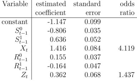
The resulting model Mt6 for the series (xt) has an estimated standard deviation of
0.380 for the main random effect, an estimated standard deviation of 0.317 for the interac-tion random effect, and estimated regression coefficients as given in Table 5 together with their standard errors. The corresponding odds ratios for the binary regressor variables
Yt and Zt are also given in Table 5. The model Lk6 for the series (yt) has an estimated
standard deviation of 0.367 for the main random effect, an estimated standard deviation of 0.459 for the interaction random effect, and estimated regression coefficients as given in Table 6 together with standard errors and odds ratios. It has been noted, for example
by Hartzel et al. (2001), p. 91, that the kind of algorithm used in thelmer function may
lead to serious bias in the estimates of the regression parameters in logistic models. In
the present case, however, given the above caveat, the coefficient 1.468 forYtin the model
as may be seen by comparing the estimated coefficients with their standard errors.
Table 5: Estimated regression coefficients and standard errors for the model Mt6 for (xt)
Variable estimated standard odds
coefficient error ratio
constant -0.477 0.087
R0
t−1 -0.823 0.037
R1
t−1 0.512 0.043
Yt 1.468 0.075 4.342
S0
t−1 0.062 0.023
S1
t−1 -0.289 0.049
Zt 0.399 0.059 1.491
Table 6: Estimated regression coefficients and standard errors for the model Lk6 for (yt)
Variable estimated standard odds
coefficient error ratio
constant -1.147 0.099
St0−1 -0.806 0.035
S1
t−1 0.636 0.052
Xt 1.416 0.084 4.119
R0t−1 0.155 0.037
R1
t−1 -0.164 0.047
Zt 0.362 0.068 1.437
In both these models, the introduction of the random pericope effect significantly im-proved the fit of the model, and the further introduction of the random interaction also significantly increased the fit, although to a lesser extent. It should be noted that the usual asymptotic likelihood ratio test for fixed effects models, based on the chi-square dis-tribution, is not applicable to tests of variance components for mixed models, as discussed for example in Stram and Lee (1994) and Visscher (2006). The appropriate distribution of the test statistic is instead a mixture of chi-square distributions. The bracketed degrees of freedom in the final column of Table 3 and Table 4, calculated by simply considering the number of fitted parameters, whether for fixed effects or variance components, should be considered as a rough guide that suggest chi-square tests that are more conservative than the ones based on mixtures of chi-square distributions (see Visscher (2006), p. 493). In any case, the results here for the pericope and interaction effects are significant.
For both series, (xt) and (yt), the addition of the random effects significantly improved
the fit of the model, but in neither case did it have any impact on the conclusion that there is a very significant statistical dependence between whether a word is retained in Matthew and whether it is retained by Luke.
In summary, on examining Table 3, we see that in the models from Mt3 onwards,
[image:16.595.187.412.339.473.2]factor for pericope are introduced, there is at each step a significant improvement in fit as expressed by a significant decrease in the residual deviance, using the usual asymptotic
likelihood ratio test, but the effect of Yt on predictions of Xt is either increased or only
slightly diminished. Similarly, on examining Table 4, in the models from Lk3 onwards,
whereXtis included as a regressor variable, as additional regressor variables or the random
factor for pericope are introduced, there is at each step a significant decrease in the
residual deviance, but the effect of Xt on predictions of Yt is either increased or only
slightly diminished. In Tables 3 and 4, only a few of the best fitting models have been
presented, but in all other cases examined our comments about the effectiveness ofYtand
Xt as predictors still apply.
So it appears that there is a very strong dependence between the series (xt) and (yt)
even when allowance is made for a number of other covariates. In order to understand in more depth the nature of the dependence it is necessary to go down to the level of studying the Greek text in detail and discussing what the reasons might be for why Matthew and Luke tend to agree more often than would be expected by chance on what words of Mark to retain and what to omit or alter. This is the task of biblical scholars. Supporters of the two source hypothesis tend to argue that the dependence is due to similarities in the editorial strategies of Matthew and Luke, which are amenable to rational explanation, or to the influence of similar oral traditions that were available to both of them. Supporters of a triple-link model with Markan priority argue that it is much more natural to explain the agreements by assuming that Luke also had Matthew as a source or vice versa.
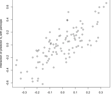
A by-product of the analysis of the models Mt6 and Lk6 is that we can examine the
interactions with the pericope factor of the predictors Yt and Xt, respectively. Figure
3 gives a scattergram of the predicted interactions for the individual pericopes. Those pericopes for which these interactions are largest in a positive direction are the ones where
the dependence between the series (xt) and (yt) appears to be the strongest. It is these
pericopes that are suggested by our analysis as the ones which in the first instance might appear to offer the most serious challenge for defenders of the two-source hypothesis and for which a detailed analysis of the text might be particularly relevant with regard to agreements between Matthew and Luke in what to retain and what to omit or alter. For example, the pericope with the largest positive interaction for both the predictors
Yt and Xt, the one in the top right hand corner of Figure 3, is Mk 1:40-45kMt 8:1-4kLk
5:12-16 on the healing of a leper. This does indeed turn out to be a pericope where the issue of disproportionally large numbers of common retentions and common omissions or alterations is readily apparent.
5
Conclusions and directions for future work
-0.3 -0.2 -0.1 0.0 0.1 0.2 0.3
-0.6
-0.4
-0.2
0.0
0.2
0.4
0.6
Interaction of predictor Yt with pericope
Interaction of predictor
Xt
[image:18.595.105.477.241.562.2]with pericope
in form, and our results are inconclusive as to whether is more likely that Matthew had Luke as a source or that Luke had Matthew as a source.
As discussed briefly in Sections 1 and 2, a hypothesis that Mark and Luke worked independently of each other could still lead to statistical dependence in the choice of words that they each retained unchanged from Mark. However, the introduction of the covariate for direct speech and of the factor for pericope in Section 4 as the most immediately obvious way of accounting for some of the statistical dependence had little effect. A statistical analysis is no substitute for the kinds of detailed textual analysis carried out by biblical scholars, but it may be helpful in clarifying certain issues and, as in the present case, raising questions that should perhaps be addressed more comprehensively than has previously been the case. How do proponents of the two-source hypothesis account for the apparently strong statistical dependence between the texts of Matthew and Luke in their use of Mark? For a statistical approach there is the question of what other ways might be found of modelling the patterns of word retention that would better illuminate or explain the statistical dependence. This might be through the construction of additional covariates that could be introduced into our models or the the exploration of other techniques for modeling binary time series such as discussed, for instance, by MacDonald and Zucchini (1997). In particular, work is in progress on the use of hidden Markov models, for which see also Zucchini and MacDonald (2009). The decoding of the text of Mark that then emerges into what is the most likely sequence of hidden states to have given rise to the observed series also suggests segments of the text that may be particularly relevant in exhibiting the apparent dependence in Matthew’s and Luke’s use of Mark.
On the other hand, we may wish to explore further the alternative hypotheses em-bodied in the two cases of the triple-link model that assume Markan priority: (i) that Matthew used Mark, but Luke used both Mark and Matthew and (ii) that Luke used Mark, but Matthew used both Mark and Luke. We may first note the results of Abakuks (2006a) and (2007) that in the simple models assumed there the first of these alternatives gives a somewhat better fit to the data. A time series analysis based on the ideas of the present paper would require the construction of a more complex database where the use of two gospels by the author of a third could be investigated. A first step in this direction is the construction of databases similar in form to the one used in the present paper but using Matthew and Luke as the base texts instead of Mark.
Beyond that, there is enormous scope for developing more sophisticated databases of the texts of the synoptic gospels, their grammatical and narrative structures and their inter-relationships, going far beyond the relatively simple idea of just recording which words are retained unchanged from one gospel to another, and then developing statis-tical tools for their analysis. Such an enterprise would, however, require major inter-disciplinary collaboration and substantial resources of time and manpower.
Acknowledgement
Appendix A
Table 7: A section (Mk 1:42-44) of the series xt, yt, zt
chapter verse word t xt yt zt
1 42 1 632 1 1 0
1 42 2 633 0 0 0
1 42 3 634 0 1 0
1 42 4 635 0 1 0
1 42 5 636 1 1 0
1 42 6 637 1 1 0
1 42 7 638 1 1 0
1 42 8 639 0 0 0
1 42 9 640 1 0 0
1 43 1 641 0 0 0
1 43 2 642 0 0 0
1 43 3 643 0 0 0
1 43 4 644 0 0 0
1 43 5 645 0 0 0
1 43 6 646 0 0 0
1 44 1 647 1 1 0
1 44 2 648 1 0 0
1 44 3 649 1 1 0
1 44 4 650 1 0 1
1 44 5 651 1 1 1
1 44 6 652 0 0 1
1 44 7 653 1 0 1
1 44 8 654 1 1 1
1 44 9 655 1 0 1
1 44 10 656 1 1 1
1 44 11 657 1 1 1
1 44 12 658 1 1 1
1 44 13 659 1 1 1
1 44 14 660 1 1 1
1 44 15 661 0 1 1
1 44 16 662 0 1 1
1 44 17 663 0 1 1
1 44 18 664 0 1 1
1 44 19 665 0 1 1
1 44 20 666 0 0 1
1 44 21 667 1 1 1
1 44 22 668 1 1 1
1 44 23 669 1 1 1
1 44 24 670 1 1 1
References
Abakuks, A. (2006a) A statistical study of the triple-link model in the synoptic problem.
J. R. Statist. Soc. A, 169, 49-60.
Abakuks, A. (2006b) The synoptic problem and statistics. Significance, 3, 153-157.
Abakuks, A. (2007) A modification of Honor´e’s triple-link model in the synoptic problem.
J. R. Statist. Soc. A, 170, 841-850.
Aland, K. (ed) (1996) Synopsis Quattuor Evangeliorum, 15th edn. Stuttgart: Deutsche
Bibelgesellschaft.
Bauckham, R. (2006)Jesus and the Eyewitnesses: The Gospels as Eyewitness Testimony.
Grand Rapids: Eerdmans.
Barr, A. (1995)A Diagram of Synoptic Relationships, 2nd edn. Edinburgh: T & T Clark.
Dunn, J. D. G. (2003a) Altering the default setting: re-envisaging the early transmission
of the Jesus tradition. New Test. Stud.,49, 139-175.
Dunn, J. D. G. (2003b)Christianity in the Making, Volume 1: Jesus Remembered. Grand
Rapids: Eerdmans.
Farmer, W. R. (1969) Synopticon: The verbal agreement between the Greek Texts of
Matthew, Mark and Luke contextually exhibited. Cambridge: Cambridge University Press.
Goodacre, M. (2001)The Synoptic Problem: A Way Through the Maze. London: Sheffield
University Press.
Goodacre, M. (2002) The Case Against Q: Studies in Markan Priority and the Synoptic
Problem. Harrisburg, PA: Trinity Press International.
Goodacre, M. and Perrin, N. (eds.) (2004) Questioning Q. London: SPCK.
Granger, C. W. J. (1969) Investigating causal relations by econometric models and
cross-spectral methods. Econometrica,37, 424-438.
Hartzel, J, Agresti, A. and Caffo, B. (2001) Multinomial logit random effects models.
Statistical Modelling ,1, 81-102.
Hengel, M. (2000) The Four Gospels and the One Gospel of Jesus Christ. London: SCM
Press.
Honor´e, A. M. (1968) A statistical study of the synoptic problem. Nov. Test.,10, 95-147.
Huck, A. (1949) Synopsis of the First Three Gospels, 9th edn. Oxford: Blackwell.
Kedem, B. and Fokianos, K. (2002)Regression Models for Time Series Analysis. Hoboken:
Wiley.
Kloppenborg, J. S. (2008) Q, the earliest Gospel: an introduction to the original stories
and sayings of Jesus. Louisville: Westminster John Knox Press.
McCullagh, R. E. and Nelder, J. A. (1989)Generalized Linear Models, 2nd edn. London:
Chapman & Hall.
MacDonald, I. L. and Zucchini, W. (1997)Hidden Markov and Other Models for
Discrete-valued Time Series. London: Chapman & Hall.
M¨achler, M. and B¨uhlmann, P. (2004) Variable length Markov chains: methodology,
computing, and software. Journal of Computational and Graphical Statistics, 13,
435-455.
Morgenthaler, R. (1971)Statistische Synopse. Z¨urich/Stuttgart: Gotthelf-Verlag.
Mosconi, R. and Seri, R. (2006) Non-causality in bivariate binary time series. Journal of
Econometrics, 132, 379-407.
Nestle, E. and Aland, K. (eds) (1963)Novum Testamentum Graece, 25th edn. Stuttgart:
Poirier, J. C. (2008) Statistical studies of the verbal agreements and their impact on the
synoptic problem. Currents in Biblical Research, 7, 68-123.
Stram, D. O. and Lee, J. W. (1994) Variance components testing in the longitudinal
mixed effects model. Biometrics, 50, 1171-1177.
Tyson, J. B. and Longstaff, T. R. W. (1978)Synoptic Abstract: Volume XV of the
Com-puter Bible. Wooster, OH: Biblical Research Associates.
Visscher, P. M. (2006) A note on the asymptotic distribution of likelihood ratio tests to
test variance components. Twin Research and Human Genetics, 9, 490-495.
Yee, T. W. and Wild, C. J. (1996) Vector generalized additive models. J. R. Statist. Soc.
B, 58, 481-493.
Zucchini, W. and MacDonald, I. L. (2009) Hidden Markov Models for Time Series: An

![2009 POC Reverse Engineering Contest [linz] pdf](data:image/gif;base64,R0lGODlhAQABAIAAAP///wAAACH5BAEAAAAALAAAAAABAAEAAAICRAEAOw==)