A ROBUST FRAMEWORK TO DETECT MOVING VEHICLES IN DIFFERENT ROAD CONDITIONS IN INDIA

98

LANDSAT 8 SATELLITE IMAGERY ANALYSIS

FOR RICE PRODUCTION ESTIMATES

(CASE STUDY : BOJONEGORO REGENCYS)

BANGUN MULJO SUKOJO1_{, SALWA NABILAH}2_{, CEMPAKA ANANGGADIPA SWASTYASTU}3 1,2,3 _{Department of Geomatics Engineering, Faculty of Civil, Environment and Earth Engineering}

Institut Technology of Sepuluh Nopember, Surabaya, Indonesia Email: 1_{[email protected]}

ABSTRACT

Bojonegoro as the mainstay of rice producers in the province of East Java, have a mission to realize the dream become a national food basket. In 2012, Bulog's Bojonegoro Bulog to be the highest regional subdivisions throughout Indonesia. Seeing this potential, it is necessary to attempt to monitor the stability of agricultural production on a regular basis. By integrating the technology of remote sensing using Landsat satellite imagery 8 to identify a growth phase and forecasting models Autoregressive Integrated Moving Average (ARIMA) to predict the productivity of rice, are expected to provide a solution and ease of repeated and continuous monitoring with wide area coverage. Identify the growth phase carried out in 9 phases. Of the linear regression between growth stage rice plants with vegetation index values are used, the value of the coefficient of determination (R2) of 0.7229 for NDVI algorithms and algorithms MSAVI amounted to 0,879. Used reflectance values of wave band SWIR2 (1.57μm-1.65μm) to help distinguish each growth phase of the identification algorithm MSAVI where to phase 3, 4, 5 has a reflectance SWIR2 above 0.15, while the phases 7, 8, 9 has reflectance SWIR2 under 0.15. Forecasting process rice productivity obtained seasonal ARIMA (1,0,0) 3. So that it can be seen Forecast Figures (ARAM) rice productivity for subround III in 2013 amounted to 66.21 quintal per hectare. Results highest estimate of 169,595.385 tons for tillering phase (15 weeks ahead of harvest) and amounted 72246.878 tons for seedling phase (13-14 harvest next week). So it can be seen that when the study was conducted, Bojonegoro located in the growing season.

Keywords: ARIMA, Phase Grown Rice, Landsat 8, Rice Productivity

1. INTRODUCTION 

Rice is a crop of rice, grown in Indonesia. Rice stock management of common concern so that information regarding the stock of rice is very important to know the situation of food availability. On the other hand stocks data is needed in determining the availability of food in a region because it involves the issue of food insecurity[1].

Seeing this potential, an effort to monitor the stability of agricultural production needs to be done on a regular basis. Remote sensing technology can provide solutions and services in spatial analysis is repeated, continuous, and covers an area that is relatively wide. Thus detecting and monitoring the development of the rice plant can be done quickly.

Figures paddy production forecast has been conducted by the Central Statistics Agency (BPS)

using indirect forecasting techniques, namely through forecasting forecasting rice production and productivity of rice harvested area. From a variety of classical and modern forecasting methods that developed and is still used to predict a time series data at this time, one of them is ARIMA. Furthermore, rice production forecast figures are needed to support the government's policy in handling the issue of food.

2. MATERIALS AND METHODS 2.1. Location Research

99 2.2. Research Methodology

Broadly speaking, the stages of research conducted consisted of five stages, namely the preparatory stage is the identification of the problem, the study of literature and data collection, data processing stage, the analysis stage and the final stage of preparation of the report form. 2.2.1. Phase data processing

The data processing is carried forth in the data processing flow diagram below (Figure. 2). Explanation of the data processing flow chart is as follows:

1. Geometrically corrected image by image to image using vector maps pertampalan Bojonegoro results RBI digitized maps Indonesia (RBI) Bojonegoro scale of 1: 25,000. Ground Control Point (GCP) is used is chosen in areas that have a clear appearance.

2. Having obtained the corrected image, do the conversion process Digital Number (DN) to

reflectance Figure 2. Flowchart of Data Processing

3. The process of calculating the vegetation index is done with input reflectance data is calculated based on an algorithm of any vegetation index. The vegetation index calculated is NDVI and MSAVI.

4. Samples in the form of paddy field equal to the size of more than 30x30 meters with a growth

100 phase that is homogeneous as much as 9 kinds of phases.

5. The field survey was conducted with a range of 3 days before and after the recording date satellite imagery data. This is to avoid rapid changes in the growth of rice plants. Data taken include the coordinates of a growth phase and photo samples in the state of the pitch.

6. Then from the data growth phase and value Vegetation Index regression process is carried out using the method of linear regression and non-linear transformation according to the shape of the relationship.

7. From the relationships each vegetation index and a growth phase, selected the best model by taking into account the coefficient of determination largest and smallest RMSE. 8. The best model results obtained were then

executed on the image. After that, the cutting (cropping) cloud and cutting images using vector maps rice fields in Bojonegoro in 2012 to map the distribution of the rice crop growth stages.

9. While the data processing rice productivity, the method used for the establishment of ARIMA time series forecasting models. The data used is data sub round productivity of rice in 1997-2013. From the available data, the data selected by distasionerkan to do identification.

10.The next phase of identification is to determine the tentative ARIMA model. This is done by analyzing the behavior patterns of ACF and PACF. In this process been p which is an order / degree auto regressive (AR), d is the order / degree differencing (distinction), and q is the order / degree moving average (MA).

11.Once the model is tentatively determined, the model parameters to be estimated. In addition, the mean square residual error is an estimate of the error variance t (time) was also calculated. 12.The diagnostic test is conducted with trials and

errors, where the MSE is generated from a variety of combinations of ARIMA model can be obtained, then the ARIMA model that produces the smallest MSE value is selected, then the ARIMA model forecasting results can

be used to predict the productivity of rice sub round to -3 in 2013.

13.Once obtained an adequate model, forecast one or even several periods ahead workable 14.Validation of forecasting is done by comparing

the forecasting results obtained through ARIMA method with observational data yields the sample. Here we can see the difference between secondary data with actual data obtained from the field.

15.From the data of forecasting productivity of rice per hectare, do multiplication to the width of each growth phase. So as to obtain estimates of rice production in Bojonegoro in n weeks.

3. RESULTS

3.1. Correction Geometric and Calculation Strength of Figure (SoF) on Landsat 8 Landsat 8 satellite imagery with a spatial resolution of 30 meters dated December 26, 2013 corrected image to image using vector maps pertampalan digitized maps results RBI Indonesia (RBI) Bojonegoro scale of 1: 25,000. Projection system used is a system of Universal Transverse Mercator (UTM) Zone 49 S, with datum World Geodetic System (WGS) 1984.

From the result of execution of the geometric correction using a 15 point GCP, an error value Root Mean Square (RMS) is 0.333804 pixels. Limit of tolerance for error RMS Error value is 1 pixel [2]. So from the RMS Error value of the average obtained in the geometric correction is to qualify at less than 1 pixel. Web design GCP points above the then calculate Strength of Figure (SoF) as follows:

Total Baseline = 34

Total Points = 17

N Size = Total Baseline x 3 = 102 Parameter N = Total points x 3 = 51 U = N Size - N Parameter = 51 Large SoF = 0.1360

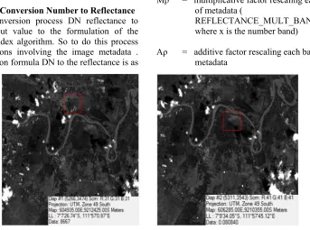
101 3.2. Digital Conversion Number to Reflectance

The conversion process DN reflectance to takes as input value to the formulation of the vegetation index algorithm. So to do this process use calculations involving the image metadata . The conversion formula DN to the reflectance is as

follows [ 3 ] :

ρλ ' = MρQcal + Aρ

Where:

ρλ ' = reflectance value , without correction angle of the sun

Mρ = multiplicative factor rescaling each band of metadata (

REFLECTANCE_MULT_BAND_x , where x is the number band)

Aρ = additive factor rescaling each band of metadata

(REFLECTANCE_ADD_BAND_x , where x is the number band)

Qcal = Digital Value Number band

3.3. Distribution of samples in each phase Grows

Figure 3. Distribution of Point GCP and Design Nets

102 In this study, samples taken randomly in several districts in Bojonegoro as many as 28 samples with steam rice growth phase conditions to mature grain elongation . Sampling was conducted on 20-22 December 2013. Of the 28 samples taken coordinate points , 4 points samples of which can not be used . Because the fourth point , cloud cover and cloud shadows in the image. As for the distribution of a growth phase samples taken are as follows.

3.4. Regression Analysis

This study tried to use pre-existing vegetation index that NDVI and MSAVI.

𝑁𝐷𝑉𝐼 𝑁𝐼𝑅 𝑅𝐸𝐷

𝑁𝐼𝑅 𝑅𝐸𝐷

𝑀𝑆𝐴𝑉𝐼 2𝑁𝐼𝑅 1 2𝑁𝐼𝑅 1 8 𝑁𝐼𝑅 𝑅𝐸𝐷

2

Where:

NIR = reflectance value near infrared spectral bands

RED = red spectral band reflectance values

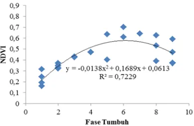
From the results of ground truth and sample coordinates growth stages of rice plants, vegetation index values obtained for each sample point a growth phase. Then do the linear regression between growth phase and vegetation index values, with the following results (Figure 6) and (Figure 7)

NDVI values obtained determination coefficient (0.7229) has a coefficient of determination under MSAVI (0,879). This is because NDVI more sensitive to chlorophyll, so that chlorophyll can confound leaf density factor. NDVI values because, in principle, based on the contrast between chlorophyll maximum absorption at a wavelength of red and maximum reflectance in the infrared due to the structure of the leaf cells.

Figure 6. Curve Regression Results Between a Growth Phase and The Vegetation Index Value NDVI

Figure 5. Distribution of The Sampling Point Phase of Growing Rice

103

Figure 7. Curve Regression Results Between a Growth Phase and The Vegetation Index Value MSAVI

NDVI is correlated with leaf area index or Leaf Area Index (LAI) [4], but NDVI have restrictions include saturation level below the tree canopy and sensitive to atmospheric conditions and ground cover [5] [6]. MSAVI pretty well used to estimate the density of the leaves, but the value of this MSAVI still sensitive to chlorophyll pigments [7].

3.5. Analysis of the Best Relationship Model MSAVI can be quite effective to approach the growth stage of rice plant which is closely related to the estimated density of the leaves. This is because the vegetation index value MSAVI background effect of soil reflectance is minimized so that the cell structure of the leaf canopy would be better [8].

In the study Kang [9], after analysis and comparison with other algorithms such as NDVI, SAVI and PVI, obtained MSAVI algorithm can not only improve the signal plants, but also greatly minimize the effects of ground cover.

But the identification using this MSAVI have the same value between phases 3, 4, 5 and 7, 8, 9 which can be seen from the curve-shaped quadratic relationship. For that utilized reflectance of wave SWIR2 (1,57μm-1,65μm) located at band 6 in Landsat 8. Wave SWIR2 used for identification foliage or leaves.

From the graph (Figure 8) can be seen that the wave reflectance value SWIR2 the rice crop will increase along with the growth of rice plants grow up to phase 4 (panicle). This is due to high humidity the plants are still green leaves are more dense and soil moisture (water content) is high. But in the 5th phase (heading) reflectance values began to decline, due to the moisture of rice plants begin to decrease due to start discharge panicles. As well as soil moisture, where the older the rice, water needs wane. But the value of reflectance

SWIR2 looks more stable at this phase in the range of values below 0.15.

Figure 8. Graph phase relationship grow and reflectance band SWIR2

Seen from the graph that for Phase 3, 4, 5 have a reflectance above 0.15 while the phases 7, 8, 9 having reflectance below 0.15.

In the study conducted Xiao et al [10], used wave SWIR (1,628μm-1,652μm) on MODIS satellite imagery in LSWI algorithm to improve soil moisture during periods of flooding and rice cultivation. But in use, is combined with the wave of a wave NIR (0,841μm- 0,875μm) to get the difference between the maximum reflectance NIR wave to the maximum absorption wave SWIR her.

3.6. Map Distribution Phase Grown Rice Based on the results of running the best relationship model that is MSAVI Landsat 8, then made a map of the distribution of rice growth phase Bojonegoro in December 2013. This map has been in tampalkan with vector maps of rice fields in Bojonegoro in 2012 in order to eliminate areas that are not fields. In addition, cloud masking process has been done to dispel the clouds.

104

Table 1. Number Size of Each Phase Growing Classification Results

No. Growing phase Area (Ha)

1. Seedling 10.912,14

2. Tillering 25.615,62

3. Stem elongation 5.259,06

4. Panicle 2.399,49

5. Heading 1.341,54

6. Flowering 235,53

7. Milk grain 1.901,52

8. Dough grain 3.415,50

9. Mature grain 7.727,04

Total Harvested Area 58.807,44

3.7. Results of Forecasting Rice Productivity Figure 10 shows the time series of data in- sample input sequence that productivity of rice crops Bojonegoro years 1997-2013 seasonal pattern with three observation periods. This is because in a year there are 3 sub round period, i.e. the period from January to April, May to August and September to December.

Box - Cox plot shows the input sequence lambda values (  ) = 1.0 and 0.89 estimate. Value

 = 1.0 indicates that the data has been stationary on the variant. When viewed from a time series plot of the input sequence, produktifias figure to be around the mean.

105

Figure 10. Time Series Plot Deret Input

Figure 11. Box-Cox Plot Deret Input

Identification of the model Autocorrelation Function ( ACF ) and Partial Autocorrelation Function ( PACF ) indicates that the ACF plot can be seen that the data also has stationary about the mean for ACF patterned down quickly ( dies down ) every 3 lag is the lag to 3 , 6 , 9 , 12 and 15. While the PACF plot shows the cut pattern on the lag 3. Therefore it can be assumed that the appropriate models are seasonal ARIMA ( 1,0,0 ) 3 .

Figure 11. Plot ACF Productivity of Paddy

Figure 12. Plot PACF Productivity of Paddy

As the model parameter estimation used the following hypotheses:

H0: Φ = 0 H1: Φ ≠ 0

Significant level: α = 0.05 Statistical Test:

Table 2. Parameters Model Test Statistic

Type Coefficient Standard Error Coefficient

T-Calc Value

P-AR

(1) 0,6244 0,1305 4,78 0,000

Model of ARIMA ( 1,0,0 ) 3 to produce P- value of 0.000 less than the significance level of 0.05, then the model is significant and H0 is rejected. However, if the diagnosis check performed to evaluate whether the ARIMA ( 1,0,0 ) 3 meet the assumption of white noise. Where white noise is a process that is independent and specific distribution with constant mean, usually assumed to be 0 and constant variance [ 11 ].

So use hypotheses: H0: ρ = 0 (white noise) H1: ρ ≠ 0 (no white noise) Significant level: α = 0.05

Statistical Test:

Table 3. Statistics Test Model for Assuming White Noise

Lag 12 24 36 48

Chi-Square 9.5 13.9 28.5 37.1

Degree of

Freedom 10 22 34 46

P-Value 0.485 0.905 0.733 0.821

It can be seen that the P-value on all lag significantly more than the level of 0.05, then failed to reject H0. It means that the model has met the assumption of white noise.

Thus the equation model for seasonal ARIMA (1,0,0) 3 are as follows :

106 Yt yt = Φ1 - 3. εt

Where :

Φ = coefficient (seasonal AR)

Yt = forecast results period - t (quintal / ha) εt = forecast error period to - t

Thus the model equations above, it can be seen from the results forecast paddy productivity T51 ( sub round III in 2013 ), namely :

Table 4. Results Forecast Figures ( ARAM ) Productivity of Rice Bojonegoro Sub Round III 2013

Forecast Upper Limit Lower Limit

66,2078 55,6237 76,7919

3.8. Productivity of Rice Based on Field Validation

Total rice production is the result of multiplying the harvested area clean with yield per hectare (productivity). Obtained the value of dry unhusked rice (GKG) of crop samples to measure 2.5m x 2.5m amounted to 3.62 kg. If an area of 6.25 m2 produce such values, it can be seen the value for the area of 1 hectare (10,000 m2). For the conversion process is carried out as follows:

10.000 m

6,25 m x 3,62 kg 5.792 kg

So it can be calculated the difference between the results of the value Forecast Figures (ARAM) and the value of the harvest samples:

ARAM - N. Sample = 66.2078 to 57.92 = 8.2878

ARAM – N. Harvest Sample = 66.2078 – 57.92 = 8.2878 quintal

Although the difference between ARAM quite large, but the value of the crop samples included in the Forecast range is between 55.6237 to 76.7919 quintal.

From the data obtained from the Central Statistics Agency (BPS) Bojonegoro, ARAM to subround III in 2013 amounted to 76.70 quintal. This is almost equal to the lower limit value of forecasting in this research that is equal to 76.80 quintal. This difference may be caused by the method used in forecasting.

Forecast model used by BPS is a simple regression model, can be linear or non-linear

(logarithmic, exponential) depending on the data pattern. Forecast production is forecast by multiplying the harvested area to forecast productivity, which has been harvested area and productivity is a result of factors that affect production. The yield per hectare obtained will represent one subround (4 months).

In this study, used Landsat 8 satellite imagery to predict the harvest area. As for predicting the productivity of rice plants used ARIMA forecasting model. This model is used by several previous studies that obtain results that the ARIMA model is a good model to use time series forecasting [12] [13].

3.9. Estimation Based on Phase Rice Production Grows Relationship with Vegetation Index MSAVI

From all the foregoing results obtained rice production estimates for the period subround III in December 2013 following the harvest forecast for the week and the future can be seen in Table 5.

This research resulted in an approximate value of rice production is based on forecasting the extent of the harvest of each phase of growth. But when seen from the side of the relationship between vegetation indices used to determine the approximate MSAVI rice productivity, there will be a different correlation.

Table 5. Estimated Production and Harvest Time

No. Growing _Phase

Estimation of Rice Production ( tons ) Estimated Harvest Time ( weeks ) 1. Seedling 72.246,878 15

2. Tillering 169.595,385 13-14

3. Stem

elongation 34.819,079

12-13

4. Panicle 15.886,495 10-11

5. Heading 8.882,041 9-10

6. Flowering 1.559,392 8-9

7. Milk grain 12.589,546 4-5

8. Dough grain 22.613,274 3-4

107 In the seedling stage until tillering MSAVI value will be low as well as the productivity of rice produced. Given in this phase, the fields are still inundated with water and ground sightings are still dominant, so that the reflectance tends to the body of water, the low value of MSAVI, so that the fields do not have the value of productivity. So that in this phase, MSAVI value can not be used to predict the productivity of rice that would be generated at the time of harvest.

In the phase of stem elongation to flowering MSAVI higher value, so the value of rice production will also be higher. So that the phase can already be used to predict the productivity of rice plants produced at harvest time. However, for better results, use MSAVI in a growth phase to mature grain milk. Because in this phase, grain begin to ripen so that forecasts the better productivity.

4. CONCLUSIONS AND RECOMMENDATIONS

From the above results, it can be concluded that the best model is obtained to identify the nine-phase growth of rice plants using algorithms MSAVI. Yields of rice samples for calculation of productivity, has the result that is within the range using ARIMA forecasting results. At the time of the study, Bojonegoro are in the growing season. This is seen by the high value of the estimated paddy production of seedling and tillering phase.

Monitoring rice productivity is very important at all times temporally to assess how the agricultural system running. Remote sensing is a technology that is ideally used given the multiple advantages such as wide coverage and fast. So with exploited remote sensing technology, this research has the advantage of monitoring method than the method used by the BPS.

As a suggestion for future research, to gain a better estimate, the selection of the image should be free or of minimal cloud cover. Or it can be used imagery with a spatial resolution smaller. As this will greatly affect the results of the calculation. Data retrieval field samples should be done with a range of 3 days before and after the recording date satellite imagery data. This is done because the rice growing relatively fast. Furthermore, this research can be developed by considering the impact of socio-economic aspects in terms of policy-making related to food security.

REFERENCES

[1] Department of Agriculture. March 27, 2013. "Food Diversification should be encouraged". <URL: http://pphp.deptan.go.id/disp_informasi/1/1/ 0/1410/lagi_lagi_soal_stok_beras.html>.Vis ited on October 8, 2013, 16:35 hours.

[2] Purwadhi, F. H. 2001. Interpretation of Digital Image. Jakarta: PT Gramedia Widiasarana Indonesia.

[3] USGS. 2013. <URL: http://Landsat.usgs.gov /band_designations_Landsat_satellites.php. Visited 18 November 2013, at 11:32.

[4] Xiao, X., et al. 2002. Landscape-scale characterization of cropland in China using Vegetation and Landsat TM images. International Journal of Remote Sensing, 23, 3579- 3594.

[5] Huete, A., et al. 2002. Overview of the radiometric and biophysical performance of the MODIS vegetation indices. Remote Sensing of Environment, 83, 195-213.

[6] Xiao, X., et al. 2003. Sensitivity of vegetation indices to atmospheric aerosols: Continental- scale observations in Northern Asia. Remote Sensing of Environment, 84, 385- 392.

[7] Haboudane, Driss et al. (2004), Hyperspectral Vegetation Indices and Novel Algorithm for Predicting Green LAI of Crop Canopie: Modelling and Validation in the Context of Precision Agriculture. Journal of Remote Sensing and Environment Vol 90 it 337-352.

[8] Sukmono, Abdi. 2013. "Estimation Model chlorophyll content and density of the leaves Rice with Hyperspectral Imagery Based on Spectral In Situ". Surabaya: Thesis Institute of Technology.

[9] Kang, Chi Hong. 1996. Methods for Collecting Information Vegetation in the Loess Plateau. Act a Beijing Botanica Sinica, 38 (1): 40-44.

multi- 

108 temporal MODIS images. Remote Sensing of Environment, 95, 480-492.

[11] Salamah, Mutiah, et al. 2003. Textbook: Time Series Analysis. Surabaya: Natural Sciences Research Institute ITS

[12] Maretha, Dedy. 2008. "Forecasting National Soybean Production and Consumption and Implications Achieving Self-Sufficiency Strategy National Soybean". Thesis Institut Pertanian Bogor.