RANDOM LINEAR NETWORK CODING BASED MULTIPATH TRAFFICS OVER HETEROGENEOUS CLOUD RADIO ACCESS NETWORK

2494

SHORT-TERM FORECASTING OF WEATHER CONDITIONS

IN PALESTINE USING ARTIFICIAL NEURAL NETWORKS

1_{IHAB HAMDAN,} 2_{MOHAMMED AWAD,}

3_{WALID SABBAH}

1_{Arab American University, Dept. of Computer Science, 240 Jenin, Palestine}

2_{Arab American University, Dept. of Computer Systems Engineering, 240 Jenin, Palestine}

3_{Arab American University, Dept. of Geographic Information Systems, 240 Jenin, Palestine}

E-mail: 1_{[email protected],} 2_{[email protected].,} 3_{[email protected]}

ABSTRACT:

Weather conditions such as quantity of the rain, daily wet or dry temperature, and humidity are important factors affecting the economy in any country. Weather forecasting departments in Palestine use linear statistical methods for forecasting daily, monthly, and yearly weather parameters. This research introduced a non-linear model to forecast daily, monthly, and yearly weather conditions which provided a much more efficient method for weather forecasting compared to the traditional linear statistical methods. This proposed non-linear forecasting model can help predict more accurate results so that meteorology and weather departments can organize their data and put the right plans to maintain the correct progress in their works. The proposed model has the ability to analyze previous weather condition patterns and use them to forecast future weather conditions. The collected weather datasets which consist of daily mean values for the three previous years in Palestine were used as targets for Multilayer Perceptron Feed-Forward Backpropagation Neural Networks (MLPFFNNBP) to forecast the future weather conditions. The dataset of rain quantity in this work consists of preprocessed mean values for ten years. The proposed model is constructed using the corresponding dataset and learning neural network to forecast weather conditions in the north region of the West Bank, Palestine which contributes to the improvement of agricultural plans. Running the proposed model using the previously mentioned data produced significant and accurate forecasted results with an acceptable minimum Mean Square Error (MSE).

Keywords: Artificial Neural Networks, Weather Conditions, Forecasting, Backpropagation Algorithm

1. INTRODUCTION

Most countries of the world are currently facing water challenges to get enough amounts of water and food for people. The absence of good plans and regulations in agricultural domains are the main factors of that problem [1]. Such absence of good plans is due to the absence of efficient and effective prediction mechanisms of weather conditions and plans to organize and regulate the agricultural process. The need for efficient prediction mechanisms of weather conditions in Palestine was the main driver to search for new rapid and accurate methods for weather and climate forecasting. The goal of these strategies is to enhance the agricultural sector at first priority and to secure people and their properties as well as to maintain the country's infrastructure and safety. In addition, knowing weather conditions for any region is extremely important for various fields including geography and engineering [2];

In countries such as Palestine, the agricultural field is the main resource for the economy [3]. There is a lack of sufficient information about weather conditions due to the lack of meteorological stations throughout the country which implies that there is no unified criterion and places all projects of conditioned environments in the same starting point. Nowadays, the change in weather conditions is affecting us directly and therefore we must be prepared for the weather conditions that affect our countries [4]. The meteorological changes have been very irregular due to recent climate change during the past few years [5]. Weather conditions in the north region of the West Bank are approximately the same as in other regions of Palestine. Data collected from meteorological stations in the city of Jenin in the northern West Bank, of Palestine. Such data is used as a dataset to forecast future weather conditions.

2495 systems of differential equations to perform short-term forecasting. The computing process in these systems is not enough to give local forecasts that are appropriate to the characteristics of different areas within from the same region. The daily weather data that have been taken over several years in the numerous observatories of the National Meteorology Department, where historical records are available (temperatures, rainfall, humidity, pressure, wind, etc.). The use of that information to forecast the next short-term weather conditions aimed at improving the resolution of outputs in the future. Neural networks gave excellent results in the field of estimation and prediction from certain input data that provide useful information about weather conditions [4]. For the above-stated reasons, we introduced an artificial intelligent model based on the artificial neural network optimized using modern learning algorithm. The objective is to adopt a model that depends on neural networks to forecast weather conditions such as rain, wet and dry temperature, dew point, etc. In this paper, we proposed an artificial neural networks model which is used to forecast the short-term future weather parameters in Palestine depending on the previous weather values for the past ten years. The weather datasets were taken from weather monitoring stations of the Palestinian Meteorological Department on the northern part of the West Bank, Palestine. The model uses Multilayer Perceptron Feed-Forward Neural Networks with Backpropagation Algorithm for training (MLPFFNNBP) as the forecasts tool of the future values of the weather conditions. The real data collected from the stations will be used as the target of the input which is the input values from 0-30 for month forecasting and 1-365 for year forecasting, the data is normalized between [0 1]. The MLPFFNNBP start forecasting the current output and compare it with the target output to find the mean square error (MSE), and then it increased the number of neurons by one neuron even to get the maximum number of determined iteration or the threshold value. This is an applied artificial intelligence research, which means that we use neural networks models to forecast the future weather conditions, depending on the pattern of the weather conditions in the past. This proposed artificial intelligent model is an alternative method that replaces the old and very short-term numerical forecasting methods (forecasting for one week). This applied research will help to authorities to make the suitable decisions regarding these sectors in Palestine that depends on the weather behavior. In section 2, we introduced the related work in this

field regardless of the applied region. In section 3, we presented a general overview of ANN architecture. Section 4 presents the proposed methodology MLPFFNNBP, the result and discussion will be presented in section 5, and finally, the conclusion of the paper will be presented.

2. RELATED WORKS

2496 compared with RBF, LVQ Naive Bayesian network and show that the results are better than others models.

Mohsen Hayati in [9] used ANN for a day in advance of the expected temperature. MLP is formed with 65% of the samples and tested using 35% of the samples of ten years of weather data from Iran, which is divided into four seasons like spring, summer, autumn, and winter. MLP network is used by three layers having a sigmoidal transfer function of hidden layers and a linear transfer function of the output layer. This research concludes that MLPNNs has a minimum prediction error, good performance, and accuracy of reasonable anticipation of this structure. Abhishek Kumar et al. in [10] has developed ANN model to predict the average monthly rainfall. He chose the data of Udupi, Karnataka, making eight months of data from fifty 400 entries for input and output. The data were normalized by finding the mean and standard deviation for each parameter. Then, the training is performed on 70% of the data and the remaining data 30% were used for testing and validation. The authors concluded that Learned is the best learning function for training, while the Trail is the best training function. The data used for research are huge enough so that the average value data decreased the mean square error.

Wang Yamin et al. in [11] proposed a new method based on the prediction of decomposition set wind speed empirically (EEMD) and backpropagation genetic algorithm neural network. The end of ten minutes each given the recorded wind speed is maintained for five days, a total of 721 test data. The result of these methods was more accurate than traditional GA-BP and EMD forecasting approach Saima H. et al., 2011 in [12] reviewed and evaluated different hybrid methods that are used for weather forecasting, .like; Model (ARMA), Hybrid regressive average slip rate and ANN, adaptive Neuro-Fuzzy inference system (ANFIS), Fuzzy Clustering and Type-2 Fuzzy Logic with other methods. The authors in this paper concentrate some hybrid methods are discussed with their merits and demerits. Tony Hall et al., 1999 in [13] developed ANN for the probability of precipitation (POP) and quantitative precipitation forecasting (QPF) Dallas-Fort Worth, in Texas. The networks were designed with three functions, firstly, it is separate for different hot and cold season’s network, and secondly, the use of QPF and POP and the last is the network becomes interactive, so that the network is working again with some changes. This significantly improves rainfall prediction serially, particularly in applications

requiring accurate results. The authors said QPF and POP can thus improve performance. Take into account that all models cannot predict with one hundred percent accuracy, but may reduce the accuracy error by several methods. The authors compared all techniques with precision and found that no model can be quite accurate, but it is expected near-optimal results.

The proposed model presented in this paper use MPFFNNBP to forecast the short-term future of weather conditions in Palestine depends on the previous values of the last ten years. The data will be divided into two partitions 70% for training and 30% for testing. The MPFFNNBP start forecasts the current output comparing it with the target output to find the mean square error.

3. ARTIFICIAL NEURAL NETWORKS

(ANNs)

2497

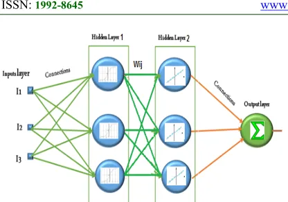
Figure 1: MLP Neural Network Architecture.

During the training phase of the network, the weights of the connections Wji that connect the hidden layers and W between the input layer and hidden layer and W from hidden to output layer are iteratively determined using the learning algorithms. From the input data, the network on each iteration produces an output, through the neurons in hidden layers, with the weights and the transfer function. This output is compared with the objective one, thus producing an error. The training concludes when the network is able to reproduce the known outputs for the input parameters. The transfer and activation functions used maybe linear, step, or sigmoid function. The second phase consists of carrying out the validation of the network designed with another set of data called test data for which the results are known, in order to verify the efficiency of the learning process. Each connection between one neuron and another is characterized by a link to a value called weights. The neurons multiply each input value from the previous layer neurons with the weights. The training process is the mapping process between the input and the output of the neural network. Then the input patterns provided to the neural network with initial weights and the output of the simple neural network is given by the following expression:

1

( )

m

ia ij j i

j

y f w x b







Where wij is the weights connection, and Xj is the value of the ith_{inputs for a simple form of the NN,} bi is the NN bias, basically it equals 1.

In general, the error of the ANNs is dependent on the difference between desired output yid and the

current output yia of the ith _{element, this error is} basically calculated using the following expression:

Er y





y

process. In this paper, we used the mean square error which can be presented by the following expression:

MSE1_n





Where n is the number of the input data (time step normally days), andϴ is the threshold value of the forecasting process. The training process continues to adjust the weights until the error criteria are satisfied regarding ϴ, the weight update is performed by the following equation:

∆ . . (4) Where α is the learning rate, normally between [0 1]. One of the advantages of the multilayer perceptron neural networks is that they can forecast any time series function. The learning process of the multilayer perceptron with backpropagation algorithm is not fixed to any application; success is to try different settings until you get the desired response. The choice of training patterns is performed depending on the explicit needs of the forecasting of weather conditions. Any changes in the patterns of training require different training parameters of the NN, but the training process remains the same [14, 4].

4. PROPOSED MODEL METHODOLOGY

Developing a methodology for weather condition forecasting must be as accurate as possible, it's clear that there is a relation between the values of future weather condition which requires the knowledge of the previous weather condition values. This belief comes from the fact that weather conditions and their values are repeated in any determined year or month for decades. Neural Networks technique used to train the weather patterns in Palestine with the aim of being able to make weather forecasts for a determined zone more efficient than the current numerical methods. The final aim is the production of a smart computer tool to forecast of the future weather data, such as rain, wet and dry temperature, dew point, etc.

The input parameters for a weather forecasting model are classified into different classes of data. Recorded daily weather conditions have many parameters known as temperature, humidity, rainfall, distance and size of the cloud, direction, and speed of the wind etc. These values are used as input to the model, xt =F(xt,…,xt-tw) + εt, where xt

is the forecasting forward steps with respect to time step t, F is the modeling function between the previous and future values, and εt is the modeling

2498 The main goal of time series is to build a model to deduce future unknown data from current data by minimizing the error function between input and output. To create an ANN model for weather forecasting, the input data should be chosen from a particular region that will be used to train the model and to test it; therefore the model will have the ability to produce correct outputs. The size of input data fed to the model can help to increase the accuracy of model results by providing an excellent level of similarity between predicted and actual output data.

The proposed model uses Multilayer Perceptron Feed Forward Neural Networks with Back Propagation (MLPFFNNBP) which depends on the following steps of training process:

 Initialize the weights of the MLPFFNNBP with random values.

 Determine input pattern Xt: (Xt1, Xt2, ...,X tn).

 Determine target output from the collected data.

To calculate the current output of the MLPFFNNBP, for the input data, we need to calculate the output values of each layer until we reach the output layer

 Calculate the forecast output of the first hidden layer of the MLPFFNNBP using the following expression:

1 1 1

1

( . )

n

L i iL

i

out f X w







 Use the output of the first layer L1 as input to the second layer L2 using the following expression:

2

1 2

1

( . )

n

L jL

j

Y f o u t w







Where f1 _{and f}2 _{are the activation functions for} output layer and hidden layer, which are calculated using the following expressions:

1 1

1 X

f

e



 (7)

f2 X (8)

 Find the error that occurs for each neuron using the following expression:

Err_L(y_id y_ia)fs'( )L (9) where Err is the error between the target output and the current output, _fs'_{( )L is the derivative of the}

activation function in each layer of the MLPFFNNBP, for the sigmoid function:

Err_L(y_idy_ia)y_ia(1y_ia) (10)

 Update the weights using the recursive algorithm, starting with the output neurons and backward until reaching the input layer, and tuning the weights in the following way:

weight value, WL (t+1) is a new weight. The

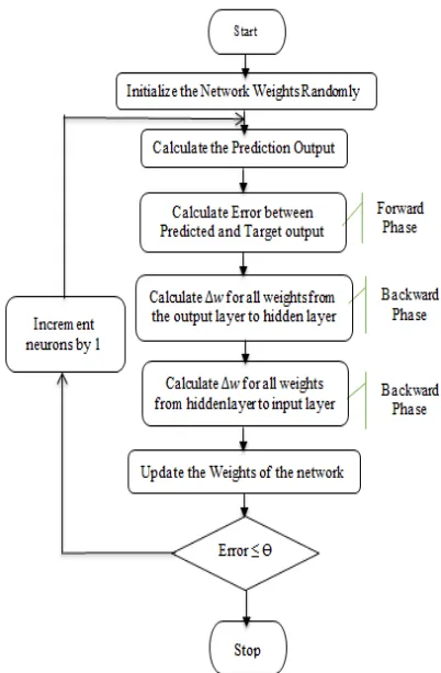
general process for MLPFFNNBP is illustrated as shown in figure 2:

Figure 2: MLPFFNNBP Methodology.

2499 structure of MLPFFNNBP on Matlab is presented in figure 3.

Figure 3: MLPFFNNBP Proposed Structure

5. RESULT AND DISCUSSION

The data set provided to the basic architecture of MLPFFNNBP model are obtained from weather records of the Palestinian Meteorological Department (PMD) in Palestine for the past 3 years (2013 to 2015). Data collection contains five weather condition parameters (maximum temperature, minimum temperature, dry temperature, wet temperature, rain quantity). Rainfall data were provided to the system in three stages yearly forecasting, monthly forecasting, and winter season forecasting. The system is simulated in MATLAB 7.1 under Windows 7 with processor i5. The result values are presented as; {# of neurons} the set of neurons used in each MLPFFNNBP. # of Iterations is the number of the execution cycle of the MLPFFNNBP. MSETrain is

the mean squared error of the training. MSETest is

the mean squared error of the testing.

1.1 Yearly Forecasting

To predict weather conditions in yearly fashion, we compute the average mean values of three years from (2013-2015) for four recorded weather condition parameters (maximum temperature, minimum temperature, dry temperature, wet temperature). The results of applying the proposed model for each of these preprocessed data as shown in figures 4 through 7 are depicted in following tables 1 through 4, respectively. Tables show the mean square error values and iterations number of training and testing are incrementally starting from 10 neurons to 100 neurons, with an incremental step of 10 neurons.

Table 1: Max Temperature Forecasting Result

# of

Neurons MSE

Train MSETest # of Iterations

10 4.24E-03 8.37E-03 16 20 3.93E-03 3.89E-03 90 30 3.37E-03 4.43E-03 17 40 2.34E-03 4.87E-03 22 50 2.22E-03 4.22E-03 22 60 2.01E-03 2.13E-03 11

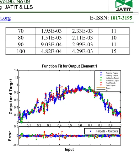
70 1.95E-03 2.33E-03 11 80 1.51E-03 2.11E-03 10 90 9.03E-04 2.99E-03 11 100 4.82E-04 4.29E-03 15

Figure 4. Best Forecasting Result of Max Temperature

From tables 1and 2 and the figures 4 and 5, we can see that the MLPFFNNBP model produce a good result of forecasting with a suitable number of neurons in the hidden layer. So the forecasting MSE after 70 neurons produces an accurate result for the future of max and min temperature.

Table 2: Min Temperature Forecasting Result.

# of

Neurons MSETrain MSETest Iterations # of

10 3.47E-03 2.6E-03 21 20 2.81E-03 3.86E-03 46 30 3.33E-03 5.34E-03 8 40 2.34E-03 4.02E-03 14 50 1.93E-03 2.65E-03 15 60 1.52E-03 3.99E-03 12 70 1.33E-03 2.39E-03 14 80 1.70E-03 3.51E-03 10 90 1.28E-03 6.22E-03 9 100 1.76E-03 3.18E-03 8

0.1 0.2 0.3 0.4 0.5 0.6 0.7 0.8 0.9 1

0 0.2 0.4 0.6 0.8 1 1.2

1.4 Function Fit for Output Element 1

O

u

tput

a

nd

Ta

rg

e

t

-0.5 0 0.5

E

rro

r

Input

Training Targets Training Outputs Validation Targets Validation Outputs Test Targets Test Outputs Errors Fit

Targets - Outputs

0.1 0.2 0.3 0.4 0.5 0.6 0.7 0.8 0.9 1 0

0.2 0.4 0.6 0.8 1 1.2

1.4 Function Fit for Output Element 1

O

u

tp

ut

a

nd

Ta

rg

et

-0.5 0 0.5

E

rro

r

Input

Training Targets Training Outputs Validation Targets Validation Outputs Test Targets Test Outputs Errors Fit

2500

Figure 5. Min Temperature forecasting Table 3: Dry Temperature forecasting Result

# of

Neurons MSETrain MSETest Iterations # of

10 3.64E-03 2.87E-03 8 20 2.41E-03 3.21E-03 16 30 1.60E-03 2.67E-03 61 40 1.35E-03 1.33E-02 16 50 1.04E-03 2.94E-03 30 60 6.63E-04 1.01E-03 19 70 5.88E-04 1.48E-03 18 80 8.05E-04 1.56E-03 9 90 4.29E-04 1.53E-03 10 100 3.00E-04 1.30E-03 25

The dry temperature is one of the most important climatic variables for the energy efficiency of buildings and for the thermal comfort of human beings. From table 3 and figures 6 we can see that the MLPFFNNBP model produced a good result of forecasting with a suitable number of neurons in the hidden layer. So the forecasting MSE after 60 neurons produced an accurate result for the future of dry temperature.

Figure 6. Best Dry Temperature Forecasting Table 4: Wet Temperature Forecasting Result

# of

Neurons MSETrain MSETest Iterations # of

10 1.00E-03 5.83E-03 27 20 1.99E-03 1.27E-03 16 30 1.77E-03 1.53E-03 11 40 1.42E-03 1.06E-03 17 50 1.17E-03 1.28E-03 16 60 1.31E-03 7.31E-04 10 70 7.17E-04 5.96E-04 23 80 6.09E-04 1.58E-03 16 90 9.15E-04 2.74E-03 9 100 1.27E-03 9.47E-04 8

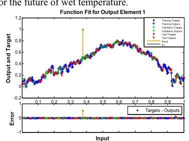
The wet temperature was used to calculate the relative humidity of the air and the temperature of dew point. From table 4 and the figure 7, we can see that the MLPFFNNBP model produced a good

result of forecasting with a suitable number of neurons in the hidden layer. So the forecasting MSE after 60 neurons produced an accurate result for the future of wet temperature.

Figure 7. Best Wet Temperature Forecasting

1.2 Monthly Forecasting

To predict weather conditions in monthly fashion, we compute the average mean values for January and August of three years from (2013-2015) for four recorded weather condition parameters (maximum temperature, minimum temperature, dry temperature, wet temperature). The results of applying the proposed model for each of these preprocessed data as shown in figures 8 through 13 are depicted in tables 5-12 respectively. Tables show the mean square error values and iterations number of training and testing in incrementally starting from 2 neurons to 20 neurons.

Tables 5: Max Temperature Forecasting for Jan.

# of Neurons

MSETrain MSETest # of

Iterations

2 4.7E-02 9.2E-02 9 4 5.3E-02 4.5E-02 7 6 9.8E-03 2.8E-02 10 8 2.6E-02 6.6E-02 7 10 1.5E-02 5.3E-02 7 12 1.1E-02 8.4E-02 7 14 9.2E-03 4.5E-02 7 16 8.9E-03 2.6E-02 7 18 9.9E-03 2.6E-02 7 20 2.5E-03 2.3E-02 9

0.1 0.2 0.3 0.4 0.5 0.6 0.7 0.8 0.9 1 -0.5

0 0.5 1

1.5 Function Fit for Output Element 1

O

u

tp

u

t a

n

d

T

a

rg

e

t

-0.2 0 0.2

E

rro

r

Input

Training Targets Training Outputs Validation Targets Validation Outputs Test Targets Test Outputs Errors Fit

Targets - Outputs

0.1 0.2 0.3 0.4 0.5 0.6 0.7 0.8 0.9 1 -0.2

0 0.2 0.4 0.6 0.8 1

1.2 Function Fit for Output Element 1

O

u

tp

ut

a

nd

T

ar

get

-1 0 1

E

rro

r

Input

Training Targets Training Outputs Validation Targets Validation Outputs Test T argets Test Outputs Errors Fit

2501

Figure 8. Best Max Temperature for Jan Forecasting.

From the result of monthly forecasting for minimum or maximum temperature as in tables 5-8 and figures 8-11, it’s clear that the proposed MLPFFNNBP model produced an accurate result for the future of maximum and a minimum temperature of two different selected months which presents a month of winter and summer. When the number of neurons is more than 15 the forecasting error improved by producing an accurate result for the future of maximum and minimum temperature

for the month.

Tables 6: Max Temperature Forecasting for Aug.

# of

Neurons MSETrain MSETest Iterations # of

2 3.3E-02 3.2E-02 8 4 3.1E-02 2.0E-02 8 6 1.1E-02 6.8E-02 8 8 2.6E-02 7.3E-02 7 10 1.3E-02 2.5E-02 10 12 1.7E-02 4.2E-02 7 14 9.9E-03 2.9E-02 7 16 1.4E-02 3.7E-02 7 18 3.5E-03 4.9E-02 7 20 1.3E-24 2.8E-02 8

Figure. 9. The best Max Temperature for Aug Forecasting.

Tables 7: Min Temperature Forecasting for Jan.

# of

Neurons MSETrain MSETest Iterations # of

2 5.98E-02 1.26E-01 12 4 6.56E-02 7.39E-02 8 6 4.11E-02 4.98E-02 11 8 4.54E-02 2.30E-02 7 10 1.37E-02 3.74E-02 9 12 2.33E-02 5.95E-02 8 14 3.68E-02 5.01E-02 7 16 8.85E-03 1.32E-01 7 18 7.53E-03 1.94E-01 7 20 3.72E-03 5.24E-02 4

Figure 10. Best Min Temperature of Jan Forecasting.

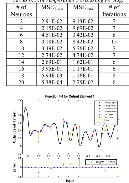
Tables 8: Min Temperature Forecasting for Aug.

# of

Neurons MSETrain MSETest Iterations # of

2 2.91E-02 9.13E-02 7 4 2.15E-02 9.69E-02 7 6 4.51E-02 3.42E-02 8 8 3.18E-02 8.42E-02 15 10 3.49E-02 5.76E-02 7 12 2.74E-02 4.74E-02 7 14 2.69E-01 1.62E-01 6 16 3.95E-01 1.17E-01 6 18 5.94E-03 1.26E-01 8 20 5.38E-04 2.75E-02 6

Figure 11. Best Min Temperature of Aug Forecasting.

0.1 0.2 0.3 0.4 0.5 0.6 0.7 0.8 0.9 1 -0.5

0 0.5 1 1.5

2 Function Fit for Output Element 1

O u tp ut a nd T a rge t -1 -0.5 0 0.5 E rro r Input Training Targets Training Outputs Validation Targets Validation Outputs Test Targets Test Outputs Errors Fit

Targets - Outputs

0.1 0.2 0.3 0.4 0.5 0.6 0.7 0.8 0.9 1

-0.2 0 0.2 0.4 0.6 0.8 1

1.2 Function Fit for Output Element 1

O u tp ut a nd T ar ge t -0.5 0 0.5 Er ro r Input Training Targets Training Outputs Validation Targets Validation Outputs Test Targets Test Outputs Errors Fit

Targets - Outputs

0.1 0.2 0.3 0.4 0.5 0.6 0.7 0.8 0.9 1 0 0.2 0.4 0.6 0.8 1 1.2

1.4 Function Fit for Output Element 1

O u tp ut a nd T a rge t -1 -0.5 0 0.5 Er ro r Input Training Targets Training Outputs Validation Targets Validation Outputs Test Targets Test Outputs Errors Fit

Targets - Outputs

0.1 0.2 0.3 0.4 0.5 0.6 0.7 0.8 0.9 1

-0.2 0 0.2 0.4 0.6 0.8 1

1.2 Function Fit for Output Element 1

O u tput a nd Ta rg e t -0.5 0 0.5 Er ro r Input Training Targets Training Outputs Validation Targets Validation Outputs Test Targets Test Outputs Errors Fit

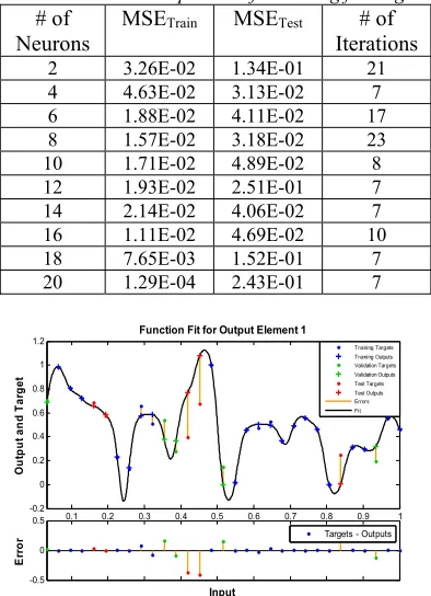
2502 The dry and wet temperature for monthly forecasting as shown in figures 12-15 and tables 9-12, it’s clear that the proposed MLPFFNNBP model produced more accurate and less MSE. This means that the model is suitable for forecasting monthly data of dry and wet temperature too.

Tables 9: Dry temperature forecasting for Jan

# of

Neurons MSETrain MSETest Iterations # of

2 3.74E-02 1.19E-01 8 4 2.90E-02 2.12E-01 9 6 3.77E-02 8.91E-02 7 8 1.86E-02 5.17E-02 9 10 4.85E-03 3.37E-02 16 12 1.41E-02 2.20E-02 7 14 6.27E-03 7.45E-02 7 16 7.56E-03 3.44E-02 7 18 8.10E-03 3.57E-01 7 20 3.22E-04 1.00E-01 6

Figure 12. The best dry temperature for Jan forecasting. Tables 10: Dry temperature forecasting for Aug

# of Neurons

MSETrain MSETest # of

Iterations

2 6.50E-02 5.58E-01 11 4 5.35E-02 6.74E-02 10 6 2.80E-02 8.40E-02 8 8 1.93E-02 2.28E-02 14 10 1.98E-03 1.31E-01 37 12 2.12E-03 6.28E-02 10 14 8.97E-03 6.33E-02 8 16 1.52E-02 3.02E-02 7 18 2.58E-04 1.27E-01 23 20 6.85E-04 4.74E-02 12

Figure 13. The best dry temperature of Aug forecasting.

Tables 11: Wet temperature forecasting for Jan

# of

Neurons MSETrain MSETest Iterations # of

2 2.64E-02 7.02E-02 14 4 8.11E-02 1.34E-01 6 6 1.42E-02 1.35E-02 9 8 2.71E-02 8.54E-02 8 10 1.04E-02 5.47E-02 7 12 3.71E-03 4.85E-02 12 14 5.73E-03 4.30E-02 8 16 9.14E-03 4.26E-02 7 18 1.97E-21 7.56E-02 94 20 5.29E-03 4.41E-02 7

Figure 14. The best-wet temperature for Jan forecasting.

Tables 12: Wet temperature forecasting for Aug

# of

Neurons MSETrain MSETest Iterations # of

2 3.26E-02 1.34E-01 21 4 4.63E-02 3.13E-02 7 6 1.88E-02 4.11E-02 17 8 1.57E-02 3.18E-02 23 10 1.71E-02 4.89E-02 8 12 1.93E-02 2.51E-01 7 14 2.14E-02 4.06E-02 7 16 1.11E-02 4.69E-02 10 18 7.65E-03 1.52E-01 7 20 1.29E-04 2.43E-01 7

Figure 14. The best-wet temperature of Aug forecasting.

0.1 0.2 0.3 0.4 0.5 0.6 0.7 0.8 0.9 1

0 0.2 0.4 0.6 0.8 1 1.2

1.4 Function Fit for Output Element 1

O u tp ut a n d Tar g et -1 -0.5 0 0.5 E rro r Input Training Targets Training Outputs Validation Targets Validation Outputs Test Targets Test Outputs Errors Fit

Targets - Outputs

0.1 0.2 0.3 0.4 0.5 0.6 0.7 0.8 0.9 1

-0.2 0 0.2 0.4 0.6 0.8 1

1.2 Function Fit for Output Element 1

O u tp u t a nd Ta rg e t -0.5 0 0.5 E rro r Input Training Targets Training Outputs Validation Targets Validation Outputs Test Targets Test Outputs Errors Fit

Targets - Outputs

0.1 0.2 0.3 0.4 0.5 0.6 0.7 0.8 0.9 1 0 0.2 0.4 0.6 0.8 1 1.2

1.4 Function Fit for Output Element 1

O u tp ut a nd T a rge t -0.5 0 0.5 E rro r Input Training Targets Training Outputs Validation Targets Validation Outputs Test Targets Test Outputs Errors Fit

Targets - Outputs

0.1 0.2 0.3 0.4 0.5 0.6 0.7 0.8 0.9 1 -0.2 0 0.2 0.4 0.6 0.8 1

1.2 Function Fit for Output Element 1

O u tput a nd Ta rg et -0.5 0 0.5 E rro r Input Training Targets Training Outputs Validation Targets Validation Outputs Test Targets Test Outputs Errors Fit

2503

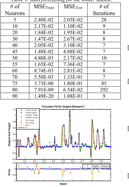
1.3 Winter Rain Forecasting

To predict rain quantity in the winter season, we computed the average mean values for November, December, January, and February months using for recorded rain values for three years (2013-2015). The results of applying the proposed model for this preprocessed data are shown in figure 13 and table 9. The table shows that the MSE values and iterations number of training and testing incrementally starting from 5 neurons to 90 neurons.

Table 9: Rain forecasting for the winter season.

# of

Neurons MSETrain MSETest Iterations # of

5 2.40E-02 2.03E-02 28 10 2.17E-02 1.10E-02 9 20 1.84E-02 1.95E-02 8 30 1.47E-02 2.67E-02 8 40 2.05E-02 3.10E-02 7 45 1.48E-02 4.88E-02 7 50 4.80E-03 2.17E-02 10 55 1.65E-02 7.36E-02 7 60 8.74E-03 2.81E-02 8 70 5.50E-03 1.33E-01 7 75 3.73E-06 1.80E-01 85 80 7.91E-09 6.54E-02 292 90 1.49E-20 1.08E-01 9

Figure 13. Best Rain forecasting for winter

6. CONCLUSION

For many reasons correspond to the necessity of creating an efficient and powerful weather condition forecasting application in Palestine, we try to pave the way of initiating an artificial intelligent forecasting model based on neural networks principles to introduce a more accurate forecasted weather condition parameters. We use preprocessed collected weather data provided by the Palestinian Meteorological Department (PMD) in West Bank, Palestine. The proposed model was used to verify the potentiality and effectiveness of model data depending on MLPFFNNBP to forecast

dry and wet temperatures, relative humidity, and rainfall. The model is easy to adapt to complex functions and able to forecast future values of weather conditions. The proposed model produced much more accurate results than using other classical methods for forecasting. The results of applying the proposed model for forecasting weather condition parameters in the north region of the West Bank in Palestine were promising and could be generalized to be used in other parts of Palestine and other similar climatic regions. This model will be transferred to the Palestinian Meteorological Department which is the official body in charge of collecting, analyzing, forecasting and reporting weather data to the public.

REFERENCES:

[1] Selonen, Vesa, Ralf Wistbacka, and Erkki Korpimäki. "Food abundance and weather modify reproduction of two arboreal squirrel species." Journal of Mammalogy, Vol 97, No. 5, 2016, pp. 1376-1384.

[2] Tripathi, Ashutosh, Durgesh Kumar Tripathi, D. K. Chauhan, Niraj Kumar, and G. S. Singh. "Paradigms of climate change impacts on some major food sources of the world: a review on

current knowledge and future

prospects." Agriculture, Ecosystems & Environment, Vol, 216, 2016,: pp. 356-373. [3] Shadeed, Sameer M., Atta ME Abboushi, and

Mohammad N. Almasri. "Developing a GIS-based agro-land suitability map for the Faria

agricultural catchment,

Palestine." International Journal of Global Environmental Vol. 16, No. 1-3, 2017, pp. 190-204.

[4] Ch.Jyosthna Devi, B.Syam Prasad Reddy, K.Vagdhan Kumar, B.Musala Reddy, N.RajaNayak, “ANN Approach for Weather Prediction using Back Propagation,” International Journal of Engineering Trends and Technology. Vol. 3 I, No.1, 2012. Pp,19-23.

[5] SYMEONAKIS, Elias. Modelling land cover change in a Mediterranean environment using Random Forests and a multi-layer neural network model. In: Geoscience and Remote Sensing Symposium (IGARSS), International. IEEE, 10-15 Jul. 2016. pp. 5464-5466.

[6] Harshani R. K. Nagahamulla, Uditha R. Ratnayake, AsangaRatnaweera,” An Ensemble of Artificial Neural Networks in Rainfall Forecasting,” The International Conference

0.1 0.2 0.3 0.4 0.5 0.6 0.7 0.8 0.9 1

-0.4 -0.2 0 0.2 0.4 0.6 0.8 1

1.2 Function Fit for Output Element 1

O

u

tp

ut

a

nd

T

a

rge

t

-1 -0.5 0 0.5

E

rro

r

Input Training Targets

Training Outputs Validation Targets Validation Outputs Test Targets Test Outputs Errors Fit

2504 on Advances in ICT for Emerging Regions -7-8 Sept. 2012: pp. 176-1-7-81.

[7] M. Nasseri, K. Asghari, M.J. Abedini, “Optimized scenario for rainfall forecasting using genetic algorithm coupled with artificial neural network,” Elsevier, ScienceDirect, Expert Systems with Applications. Vol. 35, 2008, pp. 1415–1421.

[8] R Lee, J Liu, "iJADEWeatherMAN: A Weather Forecasting System Using Intelligent Multiagent-Based Fuzzy Neuro Network", IEEE 181 Transactions on Systems, Man, and Cybernetics - Part C: Applications and Reviews, Vol 34, No 3, 2004, pp. 369 - 377.

[9] Mohsen hayati and Zahra mohebi, “Temperature Forecasting based on Neural Network Approach”, World Applied Sciences Journal Vol. 2, No. 6, 2007, pp.613-620. [10] Kumar Abhishek, Abhay Kumar, Rajeev

Ranjan, Sarthak Kumar, “A Rainfall Prediction Model using Artificial Neural Network”, IEEE Control and System Graduate Research Colloquium (ICSGRC 16-17 Jul. 2012, pp 82-87.

[11] Yamin Wang, Shouxiang Wang, Na Zhang, “A Novel Wind Speed Forecasting Method Based on Ensemble Empirical Mode Decomposition and GA-BP Neural Network”, In Power and Energy Society General Meeting 21-25 July 2013 pp. 1-5.

[12] Saima H., J. Jaafar, S. Belhaouari, T.A. Jillani, “Intelligent Methods for Weather Forecasting: A Review”, 19-20 Sept 2011 pp.1-6.

[13] Tony Hall, Harold E. Brooks, Charles A. Doswell, ” Precipitation Forecasting Using a Neural Network”, Weather and Forecasting, Vol. 14, 1999, pp. 338-345.

[14] Qasrawi, Ibrahim, and Mohammad Awad. "Prediction of the power output of solar cells using neural networks: solar cells energy sector in Palestine." Int J Comput Sci Secur IJCSS Vol. 9, No. 6, 2015, pp. 280-292.

[15] levmar- Manolis I. A. Lourakis,” A Brief Description of the Levenberg-Marquardt Algorithm Implemented”, Institute of Computer Science-Foundation for Research and Technology, Vol 4, No. 1. 2005. Pp. 1-7. [16] Awad, M., Pomares, H., Ruiz, I.R., Salameh,

O., and Hamdon, M., 2009. Prediction of Time Series Using RBF Neural Networks: A New Approach of Clustering. Int. Arab J. Inf. Technol., 6(2), pp.138-143.