BIROn - Birkbeck Institutional Research Online
Hirsch, M. and Tucker, A. and Swift, S. and Martin, Nigel and Orengo, C. and
Kellam, P. and Liu, X. (2006) Improved robustness in time series analysis of
gene expression data by polynomial model based clustering. In: Berthold,
M.R. and Glen, R.C. and Fischer, I. (eds.) Computational Life Sciences II.
Lecture Notes in Computer Science 4216. Berlin, Germany: Springer, pp.
1-10. ISBN 9783540457671.
Downloaded from:
Usage Guidelines:
Improved Robustness in Time Series Analysis of
Gene Expression Data by Polynomial Model
Based Clustering
Michael Hirsch1,, Allan Tucker1, Stephen Swift1, Nigel Martin2, Christine Orengo3, Paul Kellam4, and Xiaohui Liu1
1 School of Information Systems Computing and Mathematics, Brunel University,
Uxbridge UB8 3PH, UK
2
School of Computer Science and Information Systems Birkbeck, University of London, Malet Street, London, WC1E 7HX, UK
3
Department of Biochemistry and Molecular Biology, University College London, Gower Street, London, WC1E 6BT, UK
4
Department of Infection, University College London, Gower Street, London, WC1E 6BT, UK
Abstract. Microarray experiments produce large data sets that often contain noise and considerable missing data. Typical clustering meth-ods such as hierarchical clustering or partitional algorithms can often be adversely affected by such data. This paper introduces a method to over-come such problems associated with noise and missing data by modelling the time series data with polynomials and using these models to clus-ter the data. Similarity measures for polynomials are given that comply with commonly used standard measures. The polynomial model based clustering is compared with standard clustering methods under differ-ent conditions and applied to a real gene expression data set. It shows significantly better results as noise and missing data are increased.
1
Introduction
Microarray experiments are widely used in medical and life science research [11]. This technology makes it possible to examine the behaviour of thousands of genes simultaneously. Moreover, microarray time series experiments provide an insight into the dynamics of gene activity as an essential part of cell processes.
Despite efforts to produce high quality microarray data, such data is often burdened with a considerable amount of noise. Attempts to reduce the noise are manifold, including intelligent experimental design, multiple repeats of the experiment and noise reduction techniques in the data preprocessing [13]. In addition to the noise problem, parts of the data often can not be retrieved properly so that the dataset contains missing values. For example, a dataset of several experiments with yeast (about 500,000 values) [10] has more than 11% missing values.
This work is in part supported by the BBSRC in UK (BB/C506264/1).
M.R. Berthold, R. Glen, and I. Fischer (Eds.): CompLife 2006, LNBI 4216, pp. 1–10, 2006. c
With decreasing quality the direct clustering (DC) of the data with standard methods [5] becomes less reliable. If the data has considerable missing data, the straightforward calculation of the score functions homogeneity and separation [4] for the cluster quality becomes impossible. To overcome these problems this paper suggests the modelling of the data with continuous functions. The model based clustering is done not on the original dataset directly, but on models learnt from it. The models reduce random noise and interpolate missing values, thereby increasing the robustness of clustering.
In this paper the polynomial model based clustering (PMC) is introduced. In contrast to the DC of the data, which calculates the similarity matrix directly from the data, PMC comprised of three steps: the modelling, the calculation of the similarity matrix from the models and the grouping.
2
Methods
The application of continuous functions in time series modelling is motivated by some specific assumptions. Time series result from measurements of a quantity at different time points (TP) over a certain time period. The quantity changes continuously if it could be measured at any time in the presumed time period. Measurement restrictions are due to extrinsic factors such as technical restric-tions. Moreover, if a continuous quantity has the valuexat TPaand the value yat TPb, then the quantity has any value betweenxandyat some TP between aandb. Often time series or functions have no sharp edges in the time response, i.e. they are differentiable or smooth.
Any smooth function can be approximated by the Taylor expansion, i.e. by a polynomial. Polynomials are easy to handle since basic operations can be done by simple algebraic manipulations on the parameters. Therefore polynomials are a natural choice in time series modelling. Nevertheless, other classes of functions might be used as well. Previously, polynomials have also been used in other applications of gene expression data modelling [8,12].
2.1 Modelling
Consider series of observations, yl(ti) (l = 1. . . N, i ∈ I = {1, . . . , T}), of N
quantities atT TPs. The time elapsed between two measurements atti andti+1 might be different through the series. A sub-series ofyl(ti) in which the missing
values are omitted is denoted by ˜yl(ti)i∈J, where the index setJ is the subset
ofIthat contains these time-indices, where a value is available. IfJ is equal to I, then ˜yl(ti) =yl(ti).
Polynomials have the general form
P(t) =
n
i=0
αiti , (1)
Improved Robustness in Time Series Analysis of Gene Expression Data 3
functionf(t, α0, . . . , αn),n+ 1<|J|, |J|is the number of elements in J, such
that the function Q(α0, . . . , αn) =
i∈J(f(ti, α0, . . . , αn)−y˜l(ti))
2
becomes minimal. Therefore the equations ∂Q/∂αk = 0, k = 0. . . n have to be solved.
Applying this equation to polynomials yields
n
k=0
αk
j∈J
tkj+i=
j∈J
tijy˜l(tj) i= 0, . . . , n . (2)
These aren+ 1 linear equations for the n+ 1 parametersα0, . . . , αn. To solve
these equations an inverse matrix of the (n+ 1)×(n+ 1) matrixj∈Jtkj+i has to be calculated for each distinct subsetJ of I that occurs in the data set. To avoid large numbers in the calculation and hence a loss of precision, the time series are scaled to the time interval [−1,1].
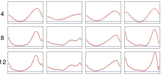
The modelling is done using polynomials with degrees ranging from 2 to 12. Figure 1 shows examples for the degrees 4, 8 and 12. With increasing degree the models fits the data better, but also may over-fit the data.
4
8
[image:4.513.76.353.261.392.2]12
Fig. 1.Modelling of gene expression data with polynomials of different degrees
2.2 Similarity Measures
To calculate the similarity between polynomials, distance measures for functions have to be used. Usually these distance measures involve integration, which re-place the sum in the equations for discrete measures. Polynomials are expandable into a Taylor-series, so that a large class of distance measures can be applied. For polynomials it is possible to calculate the anti-derivative, so that numeri-cal integration can be avoided. Each polynomial is represented by the vector of its parameters, (α0, α1, . . . , αn). Therefore the sum of two polynomials,
repre-sented by (αi) and (βi), can be written as (α0+β0, α1+β1, . . . , αn+βn) and
the anti-derivative of (αi) is represented by (0, α0,1/2α1, . . . ,1/(n+ 1)αn). The
representations for the products and derivatives of polynomials can be found analogously. Therefore, the calculation of the integrals can be reduced to some simple algebraic operations on then+ 1 parameters αi, which keeps the
derivative, the anti-derivative, the sum and the function value of polynomials takesO(n) operations, the calculation of the product of two polynomials takes O(n2) operations. For the DC the calculation effort depends on the number of TPsT. Because the number of parameters has to be considerably smaller than the number of TPs (otherwise the models would be over-fit), the calculation of the similarity matrix takes less operations for the PMC than for the DC. Two distance measures are considered, the Lp distance and the distance based on a
continuous Pearson correlation coefficient.
Lp Distance. The Lp distance is a standard distance in the space of continuous
functions and is equivalent to the p-distance (Minkowski distance) for finite dimensional spaces, such as Euclidean distance,
d(x,y) =(xi−yi)2 , (3)
or the Manhattan distance. Letx=x(t) and y=y(t) be continuous functions over the closed interval [a,b], then the Lp distance is given by
d(x,y) = p b
a
|x(t)−y(t)|pdt . (4)
Usual choices for the exponent arep= 2, which is analogous to the Euclidean distance orp= 1, which is analogous to the Manhattan distance.
Continuous Correlation Coefficient. Using the mean value theorem of calcu-lus it is possible to formulate the Pearson correlation coefficient of seriesx={xi}
andy={yi},
r(x,y) =
xiyi−N1
xi
yi
x2i −N1(xi)2 y2i −
1
N(
yi)2
, (5)
for integrable functions. Letx=x(t) andy=y(t) be continuous functions over the closed interval [a, b] andL=b−a, then the correlationrcan be calculated by
r(x,y) =
b axydt−
1
L b axdt
b aydt b
a x
2dt− 1
L( b a xdt)
2 b
ay
2dt− 1
L( b aydt)
2
. (6)
2.3 Grouping
Improved Robustness in Time Series Analysis of Gene Expression Data 5
3
Data Set
The PMC is tested with a subset of the gene expression data of the malaria intraerythrocytic developmental cycle [2]. This subset was chosen, because a functional interpretation of the genes is known and can be used to assess the clusterings. It comprises 530 genes in 14 functional groups. The gene expression is measured in 48 TPs with 1 hour time differences. The data set contained 0.32% of missing data and had a low noise level, which has been verified through [2] and by visually plotting many of the functional groups.
4
Experiments
In every experiment the clustering is done with PAM, the average-linkage method and the complete-linkage method. For DC the methods were always applied to both the Euclidean and the correlation based similarity matrix. Polynomials of degrees from 2 to 12 were fitted to each variation of the data set and both the L2 distance (4) and the correlation (6) were used for clustering. The following experiments were conducted.
1. The data set was clustered without any variations.
2. Normal distributed noise was added to the data. The standard deviation var-ied between 2% and 66% of the overall mean of the original gene expression values. The experiment was repeated 25 times.
3. The data set was changed by randomly deleting values. The number of miss-ing values varied between 2% and 50%. The experiment was repeated 25 times.
To validate the clustering results, the weightedκ(WK) method [1,7] and quotient of homogeneity and separation (H/S) [4] were used. The WK is a similarity metric between clusters, with possible values between -1 and 1. The larger the WK value the better the agreement between the cluster results. For a clustering
C={C1, . . . , CK}and a distance measuredH/S is given by
H(C) =
K
k=1
H(Ck) = K
k=1
x∈Ck
d(x,rk)2 (7)
and
S(C) = 1≤l<k≤K
d(rj,rk)2 , (8)
whererk = 1/nk
2 4 6 8 10 12 0.1 0.2 0.3 0.4 0.5
L2L2
DC
Correlation
Euclidean
2 4 6 8 10 12
[image:7.513.54.383.52.160.2]0.1 0.2 0.3 0.4 0.5 Correlation DC Correlation Euclidean
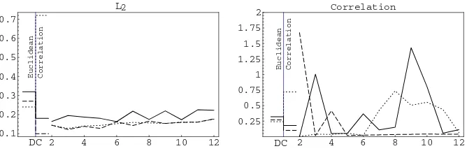
Fig. 2.Weightedκresults of DC and PMC for different similarity measures. PMC is shown depending on the degree of the model. Methods: Average Linkage – normal line, Complete Linkage – dotted line, PAM – dashed line.
5
Results
The results of the clustering of the unchanged data set for WK and H/S are shown in the Figures 2 and 3. The results of DC are marked at the left hand side of each figure, the results for PMC are shown in the main parts, one Figure for each similarity measure. The best DC result yielded the average-linkage cluster-ing of the correlation based similarity matrix,W K= 0.51 andH/S = 0.18. The PMC showed the best results when applying the average-linkage clustering to L2 similarity matrix. In particular, the models with even-numbered degrees from 4 to 10 showed constantly good values for WK (0.49) and H/S (0.16–0.19). The correlation based distance showed the best results for models with high degree, but the values for H/S were varied.
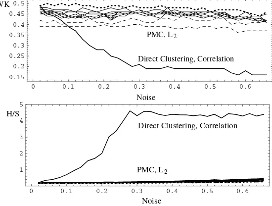
The best results in the noise experiment yielded the DC with the correlation based distance and average-linkage clustering and the PMC with L2distance and average-linkage clustering. These results are shown in Figure 4. The model of de-gree 4 is printed with a dotted line and the models of dede-gree 2 and 3 are printed with dashed lines. The other lines show the models of degrees from 5 to 12.
2 4 6 8 10 12
0.1 0.2 0.3 0.4 0.5 0.6 0.7 L2 Correlation Euclidean L2
DC 2 4 6 8 10 12
0.25 0.5 0.75 1 1.25 1.5 1.75 2 Correlation Correlation Euclidean DC
[image:7.513.52.386.448.556.2]Improved Robustness in Time Series Analysis of Gene Expression Data 7
0 0.1 0.2 0.3 0.4 0.5 0.6
0.15 0.2 0.25 0.3 0.35 0.4 0.45 0.5
PMC, L2
Direct Clustering, Correlation
Noise WK
0 0.1 0.2 0.3 0.4 0.5 0.6
1 2 3 4 5
PMC, L2
Direct Clustering, Correlation
[image:8.513.77.352.57.265.2]Noise H/S
Fig. 4.Weightedκand Homogeneity/Separation depending on the noise level (in parts of one). Cluster method: Average-linkage. Dotted line – model of degree 4, dashed lines – models of degree 2 and 3.
The PMC displayed excellent robustness, even for a high level of random noise, whereas the DC gave clearly poorer results as the noise level increased. The best choice of the model degree is 4. Models of degree 2 and 3 yielded poorer results for WK than other models, but showed consistently good H/S values. The H/S value for the model of degree 12 changed from 0.21 to 0.47, whereas the H/S value for the degree 2 model only increased from 0.17 to 0.25.
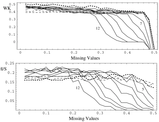
The unchanged data set has 0.32% missing values (not available values – NA). No single time series has more than 3 NAs. The best WK-results in the missing value experiment is yielded by the average linkage method with the correlation based distance for the DC and the L2 distance for the PMC, see Figure 5 top. Good results were observed using the model with degree 4 (WK 0.49–0.4; dot-ted line), which worked with up to 46% NA. The DC result is prindot-ted with a bold line and aborts at 44% NA. It runs slightly below the degree 4 model (WK 0.48–0.37). The results for the polynomials of degree 2 (WK 0.39–0.38 up to 46% NA) and 3 are very stable as well (dashed lines), but showed poorer WK val-ues. The polynomial models with higher degrees, printed with thin lines, failed sooner.
0 0.1 0.2 0.3 0.4 0.5 0
0.1 0.2 0.3 0.4 0.5
12
7
Missing Values WK
0 0.1 0.2 0.3 0.4 0.5
0.05 0.1 0.15 0.2 0.25
12 5
[image:9.513.73.350.48.261.2]Missing Values H/S
Fig. 5.Weighted κand Homogeneity/Separation of DC and PMC (degrees 2–12) de-pending on the rate of missing values. Cluster method: Average Linkage. Bold line – DC, dotted line – model of degree 4, dashed lines – models of degree 2 and 3, models of degrees 5-12 – thin lines. The H/S-value could not be calculated for the DC.
calculation of the separation. In other words, if every TP has at least one NA value the separation will be NA. Ifpis the ratio of missing values,T the number of TPs andN the number of genes, then the probability that
– a TP contains no NA is (1−p)N,
– a TP contains at least one NA is 1−(1−p)N,
– every TP contains at least one NA is (1−(1−p)N)T,
– at least one TP contains no NA is 1−(1−(1−p)N)T.
The last expression is the probability that the separation is not NA. The likeli-hood to calculate a non-NA H/S value for the considered data set is 0.9999 for 0.32% NAs, 0.2 for 1% NAs and 0.001 for 2% NAs.
On the other hand, the model based clustering allows H/S to be calculated for any number of NAs in the data, see Figure 5 bottom. Moreover, the H/S value stays stable for low degree models, between 0.16 and 0.19 for the degree 4 model, and for up to 46% missing values in the data set (method: L2, average linkage).
Improved Robustness in Time Series Analysis of Gene Expression Data 9
Homogeneity and separation could not be calculated for DC. The PMC using a model of degree 4 showed the best overall result.
6
Conclusions
This paper has introduced a novel clustering method, polynomial clustering (PMC), for dealing with missing and noisy data. It has demonstrated that PMC yielded consistently good results for different levels of noise and missing values, whereas traditional clustering methods only generated good clusters when ap-plied to high quality data. PMC showed the best robustness when using models with lower degrees, but these were too simple to reflect the features of the data set and hence yielded poorer clustering results. The models with higher degree showed better results but poorer robustness. PMC is easy to calculate. It can be used with a wide range of similarity measures and any standard clustering method.
The optimal degree of the polynomial was calculated empirically in order to balance complexity of the data with over-fitting. Future work will involve looking into ways to determine the degree automatically. The tests will be extended to other real world data sets, a wider range of distance measures and clustering techniques. It is also intended to refine the approximation technique and to analyse the modelling with other classes of functions.
References
1. Altman, D. G.: Practical Statistics for Medical Research. Chapman and Hall (1997)
2. Bozdech, Z., Llin´as, M., Pulliam, B. L., Wong, E. D., Zhu, J., DeRisi, J. L.: The
Transcriptome of the Intraerythrocytic Developmental Cycle of Plasmodium
falci-parum. PLoS Biology1(2003) 85–100
3. Eisen, M. B., Spellman, P. T., Brown, P. O., Botstein, D.: Cluster analysis and
display of genome-wide expression patterns. Proc Natl Acad Sci USA95(1998),
14863–14868.
4. Hand, D. J., Mannila, H., Smyth, P.: Principles of Data Mining. MIT Press (2001) 5. Jain, A. K., Murty, M. N., Flynn, P. J.: Data Clustering: A Review. ACM Computer
Surveys32No. 3 (1999) 264–323
6. Kaufman, L., Rousseeuw, P. J.: Clustering by means of Medoids, Y. Dodge (ed.), Statistical Data Analysis based on the L1-Norm. North-Holland, Amster-dam (1987) 405–416
7. Kellam, P., Liu, X., Martin, N., Orengo, C., Swift, S., Tucker, A.: Comparing, Contrasting and Combining Clusters in Viral Gene Expression Data. Proceedings of the IDAMAP2001 workshop, London (2001) 56–62
8. Lichtenberg, G., Faisal, S., Werner, H.: Ein Ansatz zur dynamischen Modellierung der Genexpression mit Shegalkin-Polynomen (An Approach to Dynamic Modelling
of Gene Expression by Zhegalkin Polynomials). at – Automatisierungstechnik53
9. Ralston, A.: A First Course in Numerical Analysis. McGraw-Hill (1965)
10. Spellman, P. T., Sherlock, G., Zhang, M. Q., Iyer, V. R., Anders, K., Eisen, M. B., Brown, P. O., Botstein, D., Futcher, B.: Comprehensive Identification of Cell Cycle-regulated Genes of the Yeast Saccharomyces cerevisiae by Microarray
Hy-bridization. Molecular Biology of the Cell 9, 3273–3297, URL
http://cellcycle-www.stanford.edu
11. Stekel, D.: Microarray Bioinformatics. Cambridge University Press (2003) 12. Vinciotti, V., Liu, X., Turk, R., de Meijer, E. J., ’t Hoen, P. A. C.: Exploiting
the full power of temporal gene expression profiling through a new statistical test:
Application to the analysis of muscular dystrophy data. BMC Bioinformatics 7
183 (2006)