DEVELOPMENT AND APPLICATION OF A STAGE GATE PROCESS TO REDUCE THE UNERLYING RISKS OF IT SERVICE PROJECTS

(1)

ISSN: 1992-8645 www.jatit.org E-ISSN: 1817-3195

402

3D PLANE-BASED MAPS SIMPLIFICATION FOR RGB-D

SLAM SYSTEMS

1,2

Hakim ELCHAOUI ELGHOR, 1David ROUSSEL, 1Fakhreddine ABABSA

and 2El-Houssine BOUYAKHF

1

IBISC Lab, Evry Val d'Essonne University, Evry, France 2

LIMIARF Lab, Mohammed V University Rabat, Faculty of Sciences Rabat, Morocco

E-mail: 1{Hakim.ElChaoui, David.Roussel, Fakhr-Eddine.Ababsa}@ibisc.univ-evry.fr, 2

[email protected]

ABSTRACT

RGB-D sensors offer new prospects to significantly develop robotic navigation and interaction capabilities. For applications requiring a high level of precision such as Simultaneous Localization and Mapping (SLAM), using the observed geometry can be a good solution to better constrain the problem and help improve indoor 3D reconstruction. This paper describes an RGB-D SLAM system benefiting from planes segmentation to generate lightweight 3D plane-based maps. Our aim here is to produce global 3D maps composed only by 3D planes unlike existing representations with millions of 3D points. Besides real-time trajectory estimation, the proposed method segments each input depth image into several planes, and then merges the obtained planes into a 3D plane-based reconstruction. This allows to avoid the high cost 3D point-based maps as RGB-D data contain a large number of points and significant redundant information. Our algorithm guarantees a geometric representation of the environment so these kinds of maps can be useful for indoor robot navigation as well as augmented reality applications.

Keywords: RGB-D SLAM systems, Pose Estimation, 3D Planar Features, 3D Planar Maps.

1. INTRODUCTION AND BACKGROUND

The problem of Simultaneous Localization and Mapping (SLAM) describes the process of a robot simultaneously building a map of its unknown environment and localizing within this map while exploring the environment. This problem has been a highly active field of robotics research in the last two decades. Depending on used sensors and desired world representation, several approaches have been proposed. Thus, it continues to receive further interest especially since the emergence of low-cost RGB-D Cameras. Due to dual information that it records (color and depth images), these sensors have been a topic of intensive research. Proposed works using RGB-D sensors to resolve the SLAM problem have taken two main approaches: Sparse point-based SLAM systems as in [1, 2] and dense visual SLAM methods like KinectFusion and related methods [3, 4, 5]. Although the purpose is the same, the two approaches diverge in the modeling and processing.

Dense RGB-D SLAM systems, commonly based on sophisticated equipment, such as high performance graphics hardware, were introduced by Newcombe

et al. in the well-known Kinect Fusion [3, 6]. It is a real-time dense mapping voxel-based system which integrates all depth measurements into a volumetric data structure to create highly detailed maps. However, high memory consumption restricts the system to small workspaces and the algorithm presents failures in environments with poor structure. To overcome these limitations, Whelan et al. proposed a moving volume method [4] as an extension to KinectFusion. By moving the voxel grid with the current camera pose, they overcome the restricted area problem in real-time. Keller et al.

(2)

403 specialized hardware such as GPU which may not be available on the chosen platform.

Unlike previous systems, sparse feature-based SLAM approaches are based on visual odometry. To estimate transformations between poses, these systems use visual features correspondences with a registration algorithm as RANSAC [8] or ICP. The algorithm developed by Henry et al. [1] was one of the first RGB-D systems which use visual features in combination with GICP [9] to create and optimize a pose graph SLAM and represent the environment by surfels [10]. A Graph-Based SLAM modeling [11] consists in constructing a graph which nodes are sensors poses and where edge between two nodes represents the transformation (egomotion) between these poses. This formulation enables a graph optimization step which aims to find the best nodes configuration that produces a correct topological trajectory and easier loop-closures detection when revisiting the same areas. Following the same path, Endres et al. [2] proposed a graph-based RGB-D SLAM which became very popular among Robotic Operating System (ROS) users due to its availability (wiki.ros.org/rgbdslam). This system is also a graph-based SLAM. The implementation and optimization of the pose-graph is performed by the G2o framework [12], and to represent the environment, 3D occupancy grid maps are generated using the OctoMapping approach [13]. This algorithm offers a good trade-off between the quality of pose estimates and computational cost. Typically, sparse SLAM approaches are fast due to the sensor’s egomotion estimation based on sparse points. In addition, such a lightweight implementation can be embedded easily on mobile robots and small devices such as a Turtlebot robot (www.turtlebot.com). However, the reconstruction quality is limited to a sparse set of 3D points. This leads to many redundant and repeated points in the map and lacks semantic description of the environment.

Recently, perceiving the geometry of environmental surrounding robots has become a research field of great interest in computer vision. Indeed, the use of some geometric assumptions is a crucial prerequisite for robots applications especially augmented and virtual reality or mobile robot navigation. In such applications, the role of SLAM systems progressed beyond pure localization towards generating 3D models of the environment. Current RGB-D SLAM systems begin to pay a significant interest to geometric primitives in order to build three-dimensional (3D) structure. As they are extremely common for indoor environments and

easily deduced from point clouds, 3D planes can be relevant. Thus, several works tend to use them as primitives to improve localization and mapping results. Indeed, using planes instead of raw point clouds has several advantages including data reduction, fast matching, and fast rendering in visualization.

One of the earliest RGB-D SLAM approaches incorporating planes has been developed by Trevor

et al. [14]. They combined a Kinect sensor with a large 2D planar laser scanner to generate both lines and planes as features in a graph based representation. Data association is performed by evaluating the joint probability over a set of interpretation trees of the measurements seen by the robot at one pose. Taguchi et al. [15] presented a real-time bundle adjustment system combining both 3D point-to-point and 3D plane-to-plane correspondences. Their system shows a compact representation but a slow camera tracking. This work was extended by Ataer-Cansizoglu et al. [16] to find point and plane correspondences using camera motion prediction. However, the constant velocity assumption used to predict the pose seems to be difficult to satisfy when using handheld camera. The RGB-D SLAM system [5] was extended by Salas-Moreno et al. [17] to enforce planarity on the dense reconstruction with application to augmented reality. In a recent work, G. Xiang and T. Zhang [18] proposed an RGB-D SLAM system based on planar features. From each detected 3D plane, they generate a 2D image and try to extract its 2D features points. These extracted points are back-projected on the depth to generate 3D features points used to estimate the egomotion with ICP. More recently, Whelan et al. [19] performed incremental planar segmentations on point clouds to generate a global mesh model consisting of planar and non-planar triangulated surfaces. In [20], the full representation of infinite planes is reduced to a point representation in the unit sphere 3. This allows parameterizing the plane as a unit quaternion and formulating the problem as a least-squares optimization of a graph of infinite planes.

(3)

404 composed of planar features (floor, walls, desks...etc.), such techniques are suitable to overcome the sensor's weakness without using a dense approach. Indeed, the low-cost sensor suffers from noisy data especially noise in depth values and missing depth data which makes pose estimation difficult in SLAM systems. Moreover, each registered point cloud from an RGB-D sensor contains 307200 points and requires 3.4 Megabytes in memory. Due to the large number of points and significant redundant information, resulting maps assembling several point clouds are featureless and require a heavy rendering process for visualization which leads to memory inefficiency. In this paper, we address these problems based on our previous work introduced in [21]. Using planar assumptions on the observed geometry, we will generate a minimal significant representation of the environment based on planes.

Our contributions in this paper are three-fold: i.We support the use of 3D planar features as an alternative to simple 3D points. ii.We propose a simple formulation to generate structured and reduced plane-based maps. iii.We show experimental results for localization and mapping using RGB-D data.

The reminder of this paper is organized as follows: In the following section we detail the core of our system. Section 3 contains experiments and results. Finally, Section 4 reports the conclusion and future works.

2. SYSTEM OVERVIEW

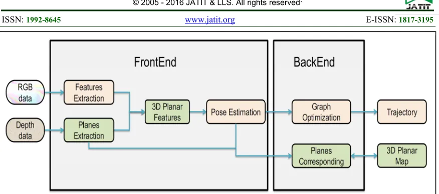
The schematic representation of our system is shown in Figure 1. Our starting point was inspired by RGB-D SLAM system introduced by Endres et al. [2]. It's a real-time graph-based SLAM using visual features. In our approach, we focus on improving RGB-D SLAM quality by taking maximum advantage of RGB-D data. We introduced 3D planar features and surfaces into the process. Our system detects 3D planes from the input data and generates a planar model of the environment by merging planes into a global map. System inputs are color images and depth maps (RGB-D data). The front end is responsible for data acquisition and association. It consists in extracting primitives from raw data and generates estimated transformations between frames. To estimate

transformations here we use 3D planar features which are the projection of 2D feature points onto 3D planes. In the backend, the graph is constructed by adding new nodes whenever a transformation between two frames exists. This transformation represents an edge between the new node and the previous one in the graph. Then, a graph optimization occurs to reduce pose estimation errors on each node. Instead of the usual map construction, we generate a global 3D planar map into which all correspondent planes will be merged.

2.1 Planes Measurements

We start by introducing planes detection and representation. Then, we discuss our 3D planar features formulation.

2.1.1 detection and representation

Planes detection is performed using only depth information by the Point Cloud Library (PCL) which extracts co-planar points sets. In our case, we are looking for planes into the full point cloud, so we perform a multi-plane segmentation with an iterative RANSAC to find the k most prominent planes. At each stage we detect the plane containing the maximum number of inliers points. Then, we remove these inliers from the point cloud and extract the next plane while the number of inliers of the new plane is still significant.

Detected planes are parameterized by = ( , , , )Т where =( , , ,) Т

is the normal vector and d is the distance from the origin.

A 3D point = ( , , ) lying on a plane satisfy the familiar plane equation + + = - , otherwise written as:

= - (1)

This equation will be used to generate our 3D planar features detailed in the next section. We also denote N the number of inliers points to a plane.

(4)

405

2.1.2 planar features

3D planar features are an alternative to the usual 3D feature points as they are projected on detected 3D planes rather than the raw depth map. The generation of these 3D planar features begins with 3D planes detection from point clouds and visual 2D feature point’s extraction from RGB images concurrently. For each 2D feature points we retrieve the depth value and check them against registered planes. 3D feature points belonging to a plane are kept and others are rejected. In addition, we performed a regularization step by projecting all kept features points satisfying a plane equation into their respective plane model.

This choice is relevant since depth maps provided by the Kinect sensor are noisy and contain missing depth values. The idea here is to benefit from 3D planes detection which could minimize 3D points measurement errors. Studies conducted in [18] and [15] agree that the planar primitives are more robust to noise. Hence, planar features are safer than the usual ones which leads to more accurate pose estimation while preserving robustness and processing time by using fewer features than raw depth maps.

2.2 Egomotion Estimation and Graph

Construction

[image:4.612.89.527.62.256.2]

Following the original method of Endres et al. [2], our system uses RGB-D data provided by the sensor to estimate camera's egomotion. The aim is to exploit these data efficiently while keeping the process fast and robust. Here we use the introduced 3D planar features for frame-to-frame transformation estimation. First of all, current frame's 2D features points descriptors are matched against already existing frames. Then, corresponding 3D planar features to the matched 2D features points in each frame are stored in two separate sets. An initial rigid transformation is estimated using these sets by a Singular Value Decomposition method [22] and refined with an iterative RANSAC. The pose graph SLAM construction begins by adding a first node when the first received frame contains enough features. Starting from this first node, a new node is added to the graph every time a transformation between two frames exists. Once the new node is added, the edge linking it to the previous one represents the estimated transformation. The constructed graph can be modeled as a nonlinear least-squares problem. This allows optimizing the graph and then finding the optimal trajectory by minimizing an error function.

(5)

406

2.3 Planes merging and Map Representation

As mentioned before, the goal is to produce lightweight 3D planar maps which can be useful for indoor robot navigation and augmented reality applications. This can be a very efficient choice for low-cost applications to avoid existing 3D point clouds representations which are highly redundant and require memory resources. Our system detects planar regions in the scene and grows planar structure in the map over time. Based on the detected planes and the estimated transformation in each added pose, this map will be constructed and updated. This is done by adding new 3D planes but also by merging the matched ones to the already mapped planes. To construct the global map, planes must be represented in the same 3D coordinates system. Let the global coordinates system be the first node added into the graph. In each node addition, we store the transformation leading to this node. As the planes detection is performed in local frames, registered planes can be transformed from the camera to world coordinates system using the egomotion obtained during the registration step. If the matrix M (Rotation R and Translation t) represents this transformation, a 3D point pw into the world coordinates can be found easily using its correspondent point in the camera pc by the well-known equation:

= + and conversely = - . If pc lies in a plane (1):

With = and = -

Then, a plane in world coordinates is defined by its normal vector and distance ( , ). Once these parameters are defined, we proceed to the matching step in order to merge the corresponding planes or add new ones in the global map. Whenever new parts of the same plane are detected and matched, we generate a new resulting plane by merging the new parts to the existing plane. If no correspondence can be found, the detected part is added to the map as a new plane. To check planes correspondence, we use a simple method. We perform a plane-to-plane comparison against all planes in the map. A detected plane is matched to an existing one if the angle and distance between them don't exceed a

threshold set successively to 10 degrees and 5cm. If a new plane matches to an already registered one , they are merged together in a new resulting plane according to their respective 3D inliers points populations Ni and

Nj by a simple linear interpolation.

To represent a plane in the map, we also need its bounding box as well as its equation. When detected in the local frame, a point cloud of inliers points to the plane is stored and then projected into the world coordinates after the egomotion estimation. Then, we proceed to a Singular Value Decomposition (SVD) of this point cloud to find its main axis vectors and consequently the bounding box according to these vectors. Once known, these bounding boxes will be used to represent the plane in the 3D global map. When the merging step happens, the bounding boxes of concerned planes are compared and the extremes are used to update the merged plane model. Even more than planes models, our map contains theoretical intersections between these planes. Planes intersections are generated using an adjacency criterion. We represent this intersection by lines and points when two or three planes intersect. This makes our map more significant and workable for other applications, and represents a first step towards a more semantic map.

3. RESULTS AND DISCUSSION

This section presents online experimental results using data acquired with a Kinect v1. Experiments were performed on a PC with Intel Core i5-2400 CPU at 3.10GHz×4. As mentioned before, planes are detected on depth maps using PCL 1.7 stable version with plane thickness threshold set to 1.5cm. All points exceeding this threshold are then rejected. The three mains planes containing at least 700 inliers points are detected on each point cloud. Detecting further planes may introduce a lot of irrelevant small planar patches. To evaluate the performances of our system we used a limited office scene mostly composed of planes. A series of experiments performed in this scene are shown in the three following subsections.

3.1 Planes quality

(6)

407 By default the resolution of Kinect images is 640×480. The resulting point cloud contains 307200 points which requires several seconds for planes detection. Hence, a subsampling step seems essential to allow online data acquisition and processing with the Kinect 30Hz update rate. This is often used by sparse systems to overcome computational time. So we used a subsampling factor λ when creating a point cloud. This subsampling factor reduces the depth image dimensions. Then, we studied the impact of subsampled data on the quality and speed of planes detection over effective distances. We performed specific experiments on a plane placed in front of the Kinect. For each distance we changed the subsampling

factor λ and observed the detected planes. Table 1 details results of these experiments. First, for each experiment, we considered runtimes for planes detection, estimated distances and the number of erroneous detected extra planes. An initial conclusion from these three columns can lead to favor the subsampling factor λ=4 considering the trade-off between runtime and planes estimation quality.

Second, we checked the impact of the number of inliers points on each detected planes. To provide more information about the quality of a plane, the average and standard deviation of the distance of its inliers points to the estimated plane model are shown. Obviously, from the

Table 1: Impact Of Subsampled Data On Planes Detection.

Effective Distance (m)

Subsampling Factor λ

Estimation Runtime (s)

Distance to the model Avg ± Std. Dev

Estimated Distance (m)

Number of Erroneous detected planes

1.5

1 2.37 0.004m ± 0.003m 1.49 0

2 0.23 0.004m ± 0.003m 1.48 0

4 0.07 0.004m ± 0.003m 1.49 0

2.5

1 7.26 0.006m ± 0.004m 2.44 1

2 1.78 0.006m ± 0.004m 2.41 2

4 0.40 0.006m ± 0.004m 2.41 0

3.5

1 7.57 0.006m ± 0.003m 3.32 2

2 1.72 0.006m ± 0.004m 3.37 1

[image:6.612.89.534.50.513.2]

4 0.40 0.007m ± 0.004m 3.36 0

Figure 2: Variations In The Number Of Inliers Points (Of The Detected Plane) According To The Factor Λ

And Distance From The Camera.

Figure 3: Variations In The Number Of Planar Features According To The Factor Λ And Planes

(7)

408 same distance, results are similar for all detected planes even if the number of inliers decreases over subsampling (Figure 2). Moreover, this number doesn't affect the estimated distance.

Nevertheless, the number of inliers 3D feature points is inversely proportional to the distance from the plane (Figure 3). Finally, we can notice that planes detection quality decreases with the distance as the depth noise becomes greater than the plane thickness threshold. As the depth noise increases with distance, planes detection over 3.5m cannot be performed. Analysis of these results allowed us to choose subsampling data with factor 4 as it doesn't degrade the detected planes quality and enables real time processing. We also notice that angles errors between detected planes do not exceed 6 degrees in any case.

3.2 Planar features and motion estimation

Accuracy of generated trajectories and runtimes of our approach was evaluated against benchmark data in our previous work [21] (Section 4.1 Benchmark datasets). Evaluations have shown that we significantly reduced the egomotion run-time while keeping a good accuracy of the estimated trajectories over the compared approaches. Here we evaluated rotational errors of our system over another ground truth means provided by a graduated tripod allowing rotations around three axes. The Kinect camera was mounted on the tripod and we proceeded to several rotations in front of a plane. With each rotation we recovered the estimated rotation and checked it over the measured one. Notice that the tripod error is about 1 degree. Table 2 shows the estimated rotations against distances from the plane.

[image:7.612.91.526.70.351.2]

For each n-degrees effective rotation, we performed 30×n-degrees deviations and computed the average and standard deviation of the estimated rotations. We also exchanged the distance from the plane to define operating conditions and limits of our system. For planes close and slightly far from the camera, results show a good estimation considering the tripod error. For these planes the rotation limit is set to 45 degrees to obtain at least 8 inliers in the feature matching set in order to accurately

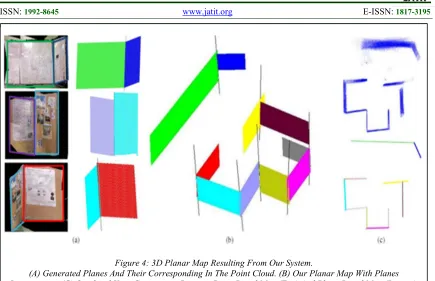
Figure 4: 3D Planar Map Resulting From Our System.

(A) Generated Planes And Their Corresponding In The Point Cloud. (B) Our Planar Map With Planes Intersections. (C) Overhead View Comparison Between Point-Based Map (Top) And Plane-Based Map (Bottom).

Table 2: Results Of Estimated Rotations Obtained With The Presented System According To The

Distance.

Rotation (Degree)

Estimated Rotation (Avg ± Std. Dev.) 1.25(m) 2.1(m) 3.3(m)

05° ± 1° 05.1° ± 0.4° 04.8° ± 0.4° 04.7° ± 0.7°

10° ± 1° 09.3° ± 0.5° 10.7° ± 0.9° 10.4°± 0.9°

20° ± 1° 19.4° ± 0.3° 19.6° ± 0.6° 19.1° ± 1.2°

30° ± 1° 30.5° ± 0.7° 30.7° ± 1.1° 29.9° ± 2.3°

(8)

409 estimate the transformations. As expected, errors of the estimated rotation increase with the distance and effective rotation. Planes located halfway to the detection distance limit (Previously estimated at 3.5m) are sensitive to camera rotations which shouldn't exceed 20 degrees. These rotations must be considerably smaller for planes closer to the distance limit. For very far planes, 45 degrees rotations cannot be achieved because it leads to detect other planes in the scene with features unmatchable with the old ones. These experiments support results obtained in our previous work concerning motion estimation accuracy using the planar features and show our system’s limits to keep good performance.

3.3 Plane-based 3D Maps

Here we show qualitative results of our 3D plane-based map for the office scene captured in real time. The Kinect was mounted on a movable support that enables it to be placed everywhere within the scene. The office scene contains 10 planes with various sizes set in different locations and features several parallel and intersecting planes. In order to compare our planar representation to the point-based maps, we kept all point clouds generated in each pose and used them to produce a global map with the SLAM RGB-D system [2]. Figure 4 shows our 3D structured planar map with intersections between planes compared to the raw point-based map.

The ratio of planar points in the whole captured point cloud is 0.57. The average number of observations for each plane is 7.1 while the average number of features for each plane is 69. Except for the rotation limit (45°) between frames, the reconstruction of this scene was not subjected to any motion or speed constraints. The average translations and rotations between poses are respectively 0.1m and 15 degrees. Planes shown in Figure 4-a (left) represent their homologous on the point cloud simultaneously generated by the system (right). Each plane model in the map was generated progressively by the merging process described before. A plane model is represented by its parameters along with its 3D bounding box. When two planes are merged, the resulting 3D bounding box is increased accordingly. Theoretical intersections are also generated between adjacent planes. Figure 4-b presents a global view of our planar map with computed

intersections. These intersections are not used yet but will ultimately be used to build a topological map of the environment. Benefiting from our minimal representation, we generated a lightweight 3D global plane-based map. Figure 4-c shows a top view of our map (bottom) compared to the raw map (top) which contains 1.363.200 3D points. In addition to its heavyweight, the lack of semantic information in such map makes it difficult to use in robotic motion planning for instance. Unlike the point-based map our structured map can be easily exploited and reused by other applications such as augmented reality and mobile navigation.

4. CONCSLUSION

(9)

410

REFRENCES:

[1] P. Henry, M. Krainin, E. Herbst, X. Ren, and D. Fox. RGB-D mapping: Using kinect-style depth cameras for dense 3D modeling of indoor environments. International Journal of Robotics Research (IJRR), 31(5):647–663, Apr. 2012.

[2] F. Endres, J. Hess, J. Sturm, D. Cremers, and W. Burgard. 3D mapping with an RGB-D camera. IEEE Transactions on Robotics, 30(1):177–187, Feb. 2014.

[3] R. A. Newcombe, S. Izadi, O. Hilliges, D. Molyneaux, D. Kim, A. J. Davison, P. Kohi, J. Shotton, S. Hodges, and A. Fitzgibbon. Kinect-fusion: Real-time dense surface mapping and tracking. In 10th IEEE International Symposium on Mixed and Augmented Reality (ISMAR 2011), ISMAR ’11, pages 127–136. IEEE Computer Society, Oct. 2011.

[4] T. Whelan, M. Kaess, H. Johannsson, M. Fallon, J. J. Leonard, and J. McDonald. Real-time large-scale dense rgb-d slam with volumetric fusion. The International Journal of Robotics Research, 34(4-5):598–626, 2015. [5] M. Keller, D. Leﬂoch, M. Lambers, S. Izadi, T. Weyrich, and A. Kolb. Real-time 3d reconstruction in dynamic scenes using point-based fusion. In Proceedings of the 2013 International Conference on 3D Vision, DV’13, pages 1–8, Washington, DC, USA, 2013. IEEE Computer Society

[6] S. Izadi, D. Kim, O. Hilliges, D. Molyneaux, R. Newcombe, P. Kohli, J. Shotton, S. Hodges, D. Freeman, A. Davison, and A. Fitzgibbon. Kinectfusion: Real-time 3d reconstruction and interaction using a moving depth camera. In Proceedings of the 24th Annual ACM Symposium on User Interface Software and Technology, UIST ’11, pages 559–568, New York, NY, USA, Oct. 2011. ACM.

[7] S. Rusinkiewicz and M. Levoy. Efﬁcient variants of the ICP algorithm. In Proceedings of the Third International Conference on 3D Digital Imaging and Modeling, (3DIM 2001), pages 145 152, May 2001.

[8] M. A. Fischler and R. C. Bolles. Random sample consensus: a paradigm for model ﬁtting with applications to image analysis and automated cartography. Communications of the ACM, 24(6):381–395, June 1981.

[9] A. Segal, D. Haehnel, and S. Thrun. Generalized-icp. In Proceedings of Robotics: Science and Systems, Seattle, USA, June 2009.

[10] H. Pﬁster, M. Zwicker, J. van Baar, and M. Gross. Surfels: Surface elements as rendering primitives. In Proceedings of the 27th Annual Conference on Computer Graphics and Interactive Techniques, SIGGRAPH ’00, pages 335–342, New York, NY, USA, 2000. ACM Press/Addison-Wesley Publishing Co. [11] G. Grisetti, R. K¨ ummerle, C. Stachniss, and

W. Burgard. A tutorial on graph-based SLAM. IEEE Intelligent Transportation Systems Magazine, 2(4):31–43, winter 2010. [12] R. K¨ ummerle, G. Grisetti, H. Strasdat, K.

Konolige, and W. Burgard. G2o: A general framework for graph optimization. In IEEE International Conference on Robotics and Automation (ICRA 2011), pages 3607–3613. IEEE, May 2011.

[13] A. Hornung, K. M. Wurm, M. Bennewitz, C. Stachniss, and W. Burgard. Octomap: An efﬁcient probabilistic 3d mapping framework based on octrees. Auton. Robots, 34(3):189– 206, Apr. 2013.

[14] A. J. B. Trevor, J. G. Rogers, and H. I. Christensen. Planar surface slam with 3d and 2d sensors. In Robotics and Automation (ICRA), 2012 IEEE International Conference on, pages 3041–3048, May 2012.

[15] Y. Taguchi, Y.-D. Jian, S. Ramalingam, and C. Feng. Point-plane SLAM for hand-held 3D sensors. In IEEE International Conference on Robotics and Automation (ICRA 2013), pages 5182–5189, May 2013.

[16] E. Ataer-Cansizoglu, Y. Taguchi, S. Ramalingam, and T. Garaas. Tracking an rgb-d camera using points anrgb-d planes. In Computer Vision Workshops (ICCVW), 2013 IEEE International Conference on, pages 51– 58, Dec 2013.

[17] R. F. Salas-Moreno, B. Glocken, P. H. J. Kelly, and A. J. Davison. Dense planar slam. In Mixed and Augmented Reality (ISMAR), 2014 IEEE International Symposium on, pages 157–164, Sept 2014.

(10)

411 [19] T. Whelan, L. Ma, E. Bondarev, P. de With,

and J. McDonald. Incremental and batch planar simpliﬁcation of dense point cloud maps. Robotics and Autonomous Systems, 69:3 – 14, 2015.

[20] M. Kaess. Simultaneous localization and mapping with inﬁnite planes. In Robotics and Automation (ICRA), 2015 IEEE International Conference on, pages 4605–4611, May 2015. [21] H. E. Elghor, D. Roussel, F. Ababsa, and E. H.

Bouyakhf. Planes detection for robust localization and mapping in rgb-d slam systems. In 3D Vision (3DV), 2015 International Conference on, pages 452–459, Oct 2015.