2016 International Conference on Computational Modeling, Simulation and Applied Mathematics (CMSAM 2016) ISBN: 978-1-60595-385-4
Oil Prices and Exchange Rates: Based on Bayesian MS-VEC Model
Sai-nan HUANG
1and Song-lin ZENG
2,*1
School of Economics, Zhongnan University of Economics and Law, 182 Nanhu Avenu, Wuhan, China
2
School of Finance, Zhongnan University of Economics and Law, 182 Nanhu Avenu, Wuhan, China
*Corresponding author
Keywords: Markov switching, Exchange rates, Oil prices, Business cycle, Asymmetric
adjustments.
Abstract. This study takes into account two crucial economic variables in its analysis of the relationship between oil prices and Rouble exchange rate, namely, nonlinear adjustment dynamics and impulse response functions. Employing a Markov-switching vector error correction model, this allows us to discriminate long-run and time-varying short-run dynamics. Our findings suggest not only that short-run adjustments of Rouble exchange rate exhibit significantly asymmetry across regimes, but also that the reverse relationship between oil price and Rouble exchange rate is mainly derived by high volatility regime, which seems closely relate to recession of Russian business cycle.
Introduction
Oil prices and exchange rates vis-à-vis U.S. dollar are two of the most important variables in international financial markets which are not only crucial for domestic economy, but also affect other economies significantly along with the globalization and financial liberalization. Recently developed countries and emerging countries suffer both large fluctuation of oil prices and volatile exchange rate, which have impact on the economic growth (see, e.g., EI Anshasy & Bradley, 2011; Lizardo & Mollick, 2010), inflation (see, e.g., Kilian & Lewis, 2011) and risk management (see, Zhang, Fan, Tsai, & Wei 2008). Taken Russia as an example, Rouble exchange rate vis-à-vis the dollar depreciate sharply by 51.23% during the period from June 2014 to January 2015 when oil prices drop heavily by 55.36%. Therefore, this study devoted to the relationship between oil price and Rouble exchange rate proves to be meaningful and necessary.
It is worth noting that most of the study on the relationship between oil prices and exchange rate are based on linear framework, such as Vector autoregressive, Granger causality test and Cointegration methodology etc. Although the endogenous issue could be solved within this linear time series approach, the periodic business cycle or financial cycle may lead to instability of the system. Thus it become necessary and meaningful to turn to a nonlinear framework, such as Markov-switching time series models, in order to capture the possible change of economy conditions often called expansion or recession. Only few paper start to account for the nonlinear relationship between oil prices and exchange rate (Beckmann & Czudaj, 2012). Moreover, most of empirical research focus on the developed countries’ exchange, such as G7 countries. Only few paper investigates emerging countries which seem to be more vulnerable to large movement of oil price or exchange rate (Turhan, Hacihasanoglu, & Soytas 2013). This paper focuses on the relationship between oil prices and Rouble exchange rate in Russia. Specifically we have tried to answer four questions: Is there any long-run cointegration relationship between oil prices and Rouble exchange rate against the dollar? Is the short-run adjustment toward equilibrium symmetric or asymmetric? Does there exist different regimes for dynamic relationship between oil prices and Rouble exchange rate against the dollar? What is the specific characteristic in each regime? By answering these questions we hope to improve understanding the relationship between oil prices and Rouble exchange rate.
also exhibit asymmetric of adjustment in the short run. Secondly, two distinct regimes, low volatility and high volatility regime, are identified by Markov-switching VECM using oil prices and Rouble exchange rate from June 1992 to April 2016. Moreover, the two regimes of low and high volatility seems to be closely related to the business cycle of expansion and recession.
The reminder of this paper is organized as follows. The following section provides a brief introduction of nonlinear methodologies, such as Markov-switching error correct mode and impulse response functions. Section 3 describes the data as well as the empirical results. Section 4 concludes.
Methodology
Noting that the oil prices (WTI) and Rouble exchange rates (Rouble) are potentially cointegrated, but their dynamic interactions may exhibit regime switching parameters, our analysis employs the following MS-VECM,
1 ( )
1 1
, 1, 2, ,
t t t
p k
t S S t k S t t
k
X
µ
X Xε
t T−
− −
=
∆ = +
∑
Γ ∆ + Π + = …(1) where p is the lag length of the MS-VAR model,[ | ~ (0, )]
t
S t
t S N Ω
ε , and
t
S
Ω is a (2×2)
positive definite covariance matrix. St presents the unobserved state or regime variable, which is
conditional on St−1 , independent of past Xs , and assumed to follow a q-state Markov process.
From the essence of economics, two-regime, that corresponds the recession-expansion cycle, is sufficient to describe the dynamic relationship between interest rates with different maturities, we thus set q=2. Hence the transition probability matrix given by
∑
= = = 2 1 1 , j ij jj ji ij ii p p p p p Pwhere pijrepresents the probability of transition from i state to j state. Besides, the MS-VECM also
allows the variance matrix
t
S
Ω to dependent on the regime variable.
The
t
S
Π matrix, which equals to '
t
t S
Sβ
α , contains the long-run relationships between short-term
and long-term interest rates ( '
t
S
β ) and the adjustment parameter when the interest rate goes beyond
the long-run relationship (
t
S
α ) in the MS-VEC model. Since this paper is aim to exam whether the adjustment of interests rates is asymmetry or not in two different regimes. This matrix
t
S
Π in this
paper is assumed as '
t t
t S S
S=α β
Π , where β is the state-independent long-run cointegration
matrix and
t
S
α are the state-dependent short-term adjustment matrix.
To estimate the MS-VECM model, the Bayesian MCMC estimation based on the Gibbs sampling is employed. The MCMC takes the regimes as distinct sets of parameter, the data augmented approach is applied to deal with the estimation issue for the latent state variables.
Data and Empirical Findings
Data
Asymmetric Adjustment across Regimes
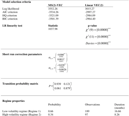
We estimate both linear VEC and MS-VEC models over the full sample period 1992:06-- 2016:04 with 285 observations. Table 1 reports estimation results and model selection criteria for the MS-VEC model given in equations (1) and (3). The lag order is selected as 2 according to the minimum AIC value in a VAR for both linear VEC and MS-VEC models. The MS-VEC model is estimated by Bayesian Monte Carlo Markov Chain (MCMC) method with Gibbs sampling.
First, we use the likelihood ratio statistic to test the nonlinearity, in which the linear VECM as the null hypothesis and MS-VECM as the alternative one. Since unidentified parameters exist under the null, the LR test is not standard. The χ2 p-values (in square brackets) with degrees of freedom equal to the number of restrictions as well as the number of restrictions plus the numbers of parameters unidentified under the null are reported, and the p-value of the Davies' test is presented in squared brackets as well. We find that the linearity is rejected. Henceforth, we focus on discussing the estimates of the nonlinear model, MS-VECM.
One of the aims of this paper is to see the asymmetrical adjustments toward the long-run equilibrium across regimes. According to the estimates of the short run correction parameters,
α
, in Table 1, we could notice that the adjustment of Rouble exchange rate exhibit significantly asymmetricity across regimes. More specifically, the speed of Rouble exchange rate adjustment to long-run equilibrium is quicker under high-volatility regime than that under low-volatility one,| | | | =2 > =1
t
t S
S α
[image:3.612.91.519.356.740.2]α . By contrast, we find no evidence supporting the asymmetricity for oil price.
Table 1. Estimation Results for the MS-VEC Model.
Model selection criteria
MS(2)-VEC Linear VEC(2)
Log likelihood 3552.26 3015.27
AIC criterion -3534.26 -2997.27
HQ criterion -3521.09 -2984.09
BIC criterion -3501.39 -2964.40
LR linearity test Statistic p-value
1037.98 2 ***
] 0000 . 0 [ ) 9 ( = χ * * * 2 ] 0000 . 0 [ ) 11 ( = χ * * * ] 0000 . 0 [ = Davies
Short run correction parameters
− = = ) 007 . 0 ( * ) 001 . 0 ( * * * 1 0011 . 0 006 . 0 t S α − − = = ) 006 . 0 ( ) 006 . 0 ( * * *
2 0.0026
028 . 0 t S α
Transition probability matrix
0.879 0.061 0.121 0.939 = P Regime properties
Probability Observations Duration
(months)
Low-volatility regime (Regime 1) 0.66 189 16.66
Two Regimes Identified from Rouble and Oil Price vs. the Business Cycle
The long-run average probabilities of a low and high-volatility regime are 0.66 and 0.34, respectively. That is, for our 287 observations, we expect the low-volatility regime to occur on 187 occasions, and 97 for high-volatility one, implying an average 16.66-month duration in the low-volatility regime and 8.26 in the high-volatility one. The actual outcomes over our sample is 233 occasions in the low-volatility regime, and 54 in high-volatility regime, which are quite close to the expectation of the MS-VECM.
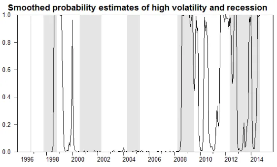
[image:4.612.166.447.227.397.2]In order to see the links between the high-low volatility regime and the recession-expansion cycle, Figure 2 plots the estimates of the smoothed probabilities of high-volatility regime (regime 2) with shaded (grey) bars that correspond to OECD business cycle recession. Visually, Figure 2 reveals a strong correspondence between the high-volatility regime and the business cycle recession.
Figure 2. Smoothed Probability Estimates of High-volatility Regime.
[image:4.612.103.508.566.601.2]Besides, as can be seen in Table 2, we conduct a comparison of the term structure regime from MS-ECM and the OECD business cycle for the entire sample period of 287 observations. The high- (low-) volatility regime occurs when its smoothed probability is larger than or equal to (less than) 0.5. Recessions and expansions depend on the OECD business cycle dates. The ratio indicates that when the economy is in high volatility regime, the probability of experiencing a recession is 53% , larger than that in the low-volatility one, 47%. By contrast, the possibility of business cycle expansion conditional on economy in the low-volatility regime, 60%, is much larger than that in the high-volatility regime, 40%. The results showed by Table 2 imply a significant relationship between recession and high-volatility regime, or between expansion and low-volatility regime.
Table 2. High- and low-volatility vs Recession and Expansion Outcomes.
Recession Expansion Count
High Volatility 28 (53%) 24 (47%) 52
Low Volatility 64 (40%) 99 (60%) 163
Conclusion
This paper investigates the dynamic relationship between oil prices and Russian Rouble exchange rate against the dollar for the period from June 1992 to April 2016 utilizing the nonlinear Markov-switching vector error correction model and regime-dependent impulse response function by Bayesian MCMC method. Large fluctuation of Rouble exchange rate against the dollar along with the movement of oil prices from June 2014 to January 2015 provide us a new opportunity to reexamine their relationship in Emerging countries.
dollar, while the adjustment toward equilibrium exhibits significantly asymmetric across different regimes. Specifically Second, two distinct regimes, which show significantly difference of volatility, are identified in the framework of Markov-switching. Moreover, these two different regimes labeled high volatility and low volatility seems closely related to the state of business cycle.
Acknowledgement
The views expressed in this paper reflect those of the authors. The usual disclaimer applies. This research has been conducted as part of the NSFC Project No. 71403295.
References
[1] Beckmann, J., & Czudaj, R. (2013). Oil prices and effective dollar exchange rates. International Review of Economics & Finance, 27(C), 621-636.
[2] Cheng, K. C. (2008). Dollar depreciation and commodity prices. IMF (ed.), 72-75.
[3] Camarero, M., & Tamarit, C. (2002). Oil prices and Spanish competitiveness: A cointegrated panel analysis. Journal of Policy Modeling, 24(6), 591-605.
[4] Chen, S., & Chen, H. (2007). Oil prices and real exchange rates. Energy Economics, 29(3), 390-404.
[5] El Anshasy, A. A., & Bradley, M. D. (2012). Oil prices and the fiscal policy response in oil-exporting countries. Journal of Policy Modeling, 34(5), 605-620.
[6] Indjehagopian, J. P., Lantz, F., & Simon, V. (2000). Dynamics of heating oil market prices in Europe. Energy Economics, 22(2), 225-252.
[7] Krugman, P. (1983). Oil and the Dollar. In Bahandari, JS & Putnam, BH (Eds.) Economic Interdependence and Flexible Exchange Rates.