University of Warwick institutional repository: http://go.warwick.ac.uk/wrap
A Thesis Submitted for the Degree of PhD at the University of Warwick
http://go.warwick.ac.uk/wrap/49612
This thesis is made available online and is protected by original copyright.
Please scroll down to view the document itself.
Vertical variation in diffusion coefficient
within sediments
by
I. D. Chandler
Thesis
Submitted to the University of Warwick
for the degree of
Doctor of Philosophy
School of Engineering
Contents
List of Figures iv
List of Tables xiii
Acknowledgments xvi
Declarations xvii
Abstract xviii
Chapter 1 Introduction 1
1.1 Aims . . . 2
1.2 Thesis outline . . . 2
Chapter 2 Background theory and Previous Work 4 2.1 Synopsis . . . 4
2.2 Hyporheic Exchange . . . 4
2.2.1 Molecular Diffusion . . . 4
2.2.2 Turbulent Diffusion . . . 6
2.2.3 Other Driving Forces . . . 9
2.2.4 Effective Diffusion . . . 10
2.3 Predicting and Modelling Hyporheic Exchange . . . 11
2.3.1 Pumping Model . . . 11
2.3.2 Slip Flow Model . . . 16
2.3.3 Effective Diffusion Scaling Relationship . . . 20
2.3.4 Transient Storage Models . . . 26
2.3.5 One Dimensional Model . . . 29
2.4 Laboratory Studies . . . 46
2.4.1 Water Column Measurements . . . 46
2.5 Field Studies . . . 82
2.6 Sediment Parameters . . . 84
2.6.1 Sediment Motion . . . 84
2.6.2 Permeability . . . 86
2.6.3 Roughness Height . . . 87
2.7 Summary and Hypothesis . . . 87
2.7.1 Hypothesis . . . 87
Chapter 3 Experimental Setup 89 3.1 Synopsis . . . 89
3.2 Experimental Development . . . 89
3.3 Re-designed Erosimeter . . . 93
3.3.1 Motor and Control System . . . 95
3.3.2 Bed Shear Velocity Calibration . . . 99
3.3.3 In-Situ Permeability Test . . . 101
3.3.4 Temperature Sensor . . . 105
3.4 Flow Visualisation . . . 108
3.4.1 Experimental Setup . . . 108
3.4.2 Analysis . . . 112
3.4.3 Results . . . 116
3.4.4 Conclusion . . . 120
3.5 Fluorometry . . . 121
3.5.1 Cyclops 7 Fluorometer . . . 122
3.5.2 Fibre Optic Fluorometer . . . 123
3.5.3 Calibration . . . 127
3.6 Sediments . . . 130
3.6.1 Porosity . . . 132
3.7 Data Acquisition . . . 133
3.8 Experimental procedure . . . 134
Chapter 4 Experimental Results and Analysis 136 4.1 Synopsis . . . 136
4.2 Raw Data . . . 136
4.2.1 Sediment Permeability . . . 139
4.3 Evaluation of Analysis Techniques . . . 141
4.3.1 Water Column . . . 141
4.3.2 In-bed Data . . . 145
4.5 In-bed Data . . . 154
4.5.1 Effects of Bed Shear Velocity . . . 159
4.5.2 Effects of Permeability . . . 163
4.5.3 Effects of Other Experimental Parameters . . . 167
4.5.4 Dimensionless Groups . . . 167
4.6 Summary . . . 170
Chapter 5 Discussion 171 5.1 Synopsis . . . 171
5.2 Experimental Data . . . 171
5.2.1 Water Column . . . 171
5.2.2 In-bed . . . 173
5.3 Depth Dependent Diffusion Coefficient Function . . . 175
5.4 1D model comparison . . . 179
5.5 Application . . . 183
Chapter 6 Conclusion 185 6.1 Use of Erosimeter . . . 185
6.2 Vertical Variation in Diffusion Coefficient . . . 186
6.3 Further Work . . . 188
Notation 191
Appendix A Schematic of original EROSIMESS-system 208
Appendix B Chandler, Pearson, Guymer, and Van-Egmond [2010] 210
Appendix C Vector fields 217
Appendix D Full Experimental Results and Parameters 226
Appendix E Further Comparison of Model Simulations and
List of Figures
2.1 Example variation of velocity at a point with time in turbulent flow 7 2.2 Reynolds’ eddy model [Chadwicket al., 2004] . . . 8 2.3 Graphical representation of pumping flow through a sinusoidal bed-form 10 2.4 Normalised head distribution and particle flow paths (stream lines)
predicted using Elliott and Brooks [1997a] model, [Dutton, 2004] . . 12 2.5 Mean velocity profiles in near-bed regions for sediment bed
experi-ments where each point represents an average of measureexperi-ments from profiles repeated for the same sediment and flow conditions. The Solid curve represents profile (2.39) with zero displacement whilst the dashed curves represent profiles with slip velocities of 2 and 4 Fries [2007] . . . 17 2.6 Pictorial representation of slip flow . . . 18 2.7 Packman and Salehin [2003] pumping model based scaling
relation-ship showing the influence of stream velocity, permeability and poros-ity of the bed sediments . . . 21 2.8 Packman and Salehin [2003] second scaling relationship showing
ex-change is proportional to the sediment size, which suggests that the permeability of the sediment bed controls exchange with both flat beds and bed-forms . . . 22 2.9 Effective diffusion scaling relationship compared against previous
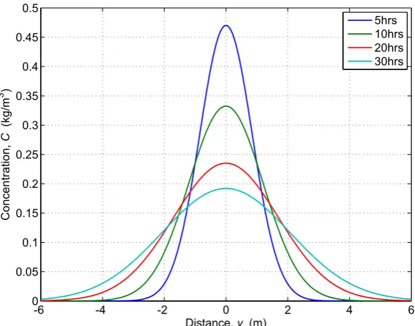
ex-perimental data [O’Connor and Harvey, 2008] . . . 25 2.10 Plane injection in an infinite domain with constant diffusion
coeffi-cient,D= 2×10⁻⁵m2/s . . . 31 2.11 Pictorial representation of method of images . . . 32 2.12 Comparison of constant and variable diffusion coefficients (D1 =
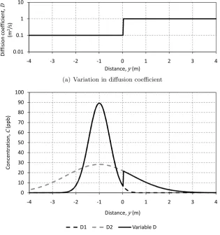
2.13 Model 3 simulation with diffusion coefficients 1×10⁻³and 4×10⁻⁷m2/s
in the regions 0< y ≤0.255m and−0.2≤y≤0m respectively . . . 39 2.14 Constant coefficient simulation solute transport between the sediment
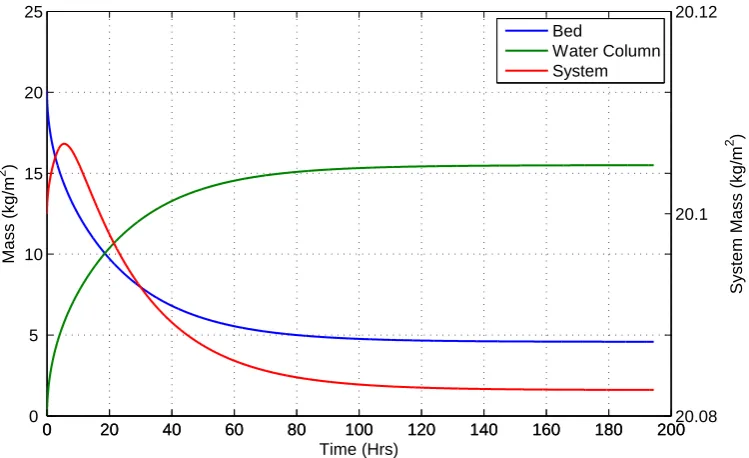
and water column using model 4 (D= 1.55×10⁻⁷m2/s) . . . 41 2.15 System and region mass from Figure 2.14 simulation showing the
small overall variation in mass during the simulation . . . 42 2.16 Simulation of solute transport between sediment and water column
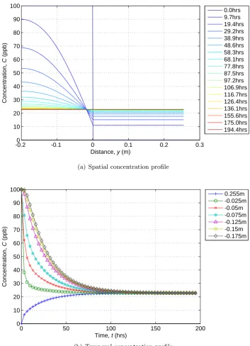
with discrete variable diffusion coefficients using model 4 . . . 44 2.17 Simulation of solute transport between sediment and water column
with continuously variable depth dependent diffusion coefficients us-ing model 4 (D= 9×10⁻⁷exp(80y)) . . . 45 2.18 Effect of using different percentages of a concentration profile on
cal-culated diffusion coefficient from model 4 water column simulated data using equation (2.100) . . . 56 2.19 Comparison of different percentages of the data taken to represent
the initial slope on Marionet al. [2002] data . . . 57 2.20 Comparison of Shimizu et al.[1990] analysis profile (generated using
(2.106)) against model 4 simulation profile used in analysis (−0.025m) 61
2.21 Comparison of Shimizu et al.[1990] analysis profile (generated using (2.106)) against 7 zone variable coefficient model 4 simulation profile used in analysis (−0.100m) . . . 62
2.22 Example analysis of 2 zone variable coefficient model 4 simulation, showing the simulation profiles used in the analysis and the result of the optimisation (red line) including the coefficient used to generate the profile (legend entry) . . . 67 2.23 Example output from Nagaoka and Ohgaki [1990] analysis of 7 zone
variable coefficient model 4 simulation with noise for the region be-tween −0.125 and −0.150m, showing the simulation profiles used in the analysis and the result of the optimisation (red line) including the coefficient used to generate the profile (legend entry) . . . 69 2.24 Pictorial representation of optimisation process indicating the ‘best’
2.25 Example optimisation from Nagaoka and Ohgaki [1990] analysis method-ology, showing the different profiles generated by the vector of diffu-sion coefficients and the focussing of the optimisation on the ‘correct’ diffusion coefficient (−0.075 and−0.100m, 7 zone model 4 simulation with noise added) . . . 71 2.26 Example output from the optimisation used in the Nagaoka and
Ohgaki [1990] analysis methodology, conducted with profiles from 7 zone model 4 simulation with noise added (−0.075 and−0.100m), showing the two profiles and the optimised analysis profile (red) (leg-end gives the profile positions, the diffusion coefficient obtained by the analysis and theRt2 value between the model simulation and the optimised analysis profiles . . . 72 2.27 Effect of sampling interval, dt, on Nagaoka and Ohgaki [1990] analysis
of 7 zone model 4 simulation (optimisation starting point Dwc =
2×10⁻⁶m2/s) . . . 74 2.28 Effect of sampling interval, dt, on Nagaoka and Ohgaki [1990] analysis
of 7 zone model 4 simulation (optimisation starting point Dwc =
2×10⁻⁷m2/s) . . . 75 2.29 Effect of a large sampling interval on Nagaoka and Ohgaki [1990]
analysis of 7 zone model 4 simulation (dt= 500s), showing the two profiles and the optimised analysis profile (red) with the legend giving the profile positions, the diffusion coefficient obtained by the analysis and the R2
t value between the model simulation and the optimised
analysis profiles . . . 76 2.30 Variation in R2t values and Nagaoka and Ohgaki [1990] analysis
pro-files with different diffusion coefficients between−0.125 and−0.150m profiles from 7 zone model 4 simulation (Equation (2.120)) . . . 78 2.31 Variation in R2t values and Nagaoka and Ohgaki [1990] analysis
pro-files with differentD1diffusion coefficients between−0.100 and−0.125m
profiles from 7 zone model 4 simulation (Equation (2.117), D2 =
2.0×10⁻⁸m2/s) . . . 79 2.32 Variation inR2t values with differentD2diffusion coefficients between
−0.100 and−0.125m profiles from 7 zone model 4 simulation (Equa-tion (2.117),D1 = 6.0×10⁻⁸m2/s) . . . 81
2.33 Variation inR2t values with differentD1 andD2 diffusion coefficients
3.1 Schematic of the erosimeter used in the initial experimental work [Chandleret al., 2010] . . . 91 3.2 Example concentration profile from test 5 from Chandleret al.[2010],
showing water column and in-bed traces with the portion of the trace used in calculating the diffusion coefficient indicated . . . 92 3.3 Initial erosimeter experimental results plotted against the O’Connor
and Harvey [2008] scaling relationship (2.51) [Chandleret al., 2010] . 92 3.4 Photograph of the complete erosimeter laboratory experimental setup 94 3.5 Schematic of the re-designed erosimeter detailing instrument
posi-tions marked . . . 95 3.6 Photograph of the motor control unit . . . 96 3.7 Change in propeller speed as the motor warms up (Dial = 300) . . . 97 3.8 Change in motor warm up time depending on length of time switched
off (Dial = 300) . . . 98 3.9 Calibration of dial reading to propeller speed (rpm) . . . 98 3.10 Results of bed shear velocity calibration relating propeller speed to
bed shear velocity . . . 101 3.11 Erosimeter permeability test setup . . . 102 3.12 Temperature correction curve for permeability test [BS1377-5, 1990] 103 3.13 Comparison of calculated (2.130) and measured permeability for
nat-ural sediment using erosimeter . . . 104 3.14 Wheatstone bridge used with temperature sensor . . . 106 3.15 Temperature sensor calibration . . . 107 3.16 Comparison of temperatures measured using an un-calibrated
labo-ratory thermometer and that given by the water bath . . . 107 3.17 Initial vertical light sheet PIV setup . . . 109 3.18 Photograph of the modified main section used in PIV experiments . 110 3.19 Horizontal Light Sheet Setup . . . 111 3.20 Example vertical light sheet calibration image showing the calibration
plate, with regular grid of dots, used by image processing software (DaVis 7.2) to convert pixel displacements to physical distance . . . 112 3.21 Evaluation of PIV image pair (left) using cross correlation resulting
in velocity vector (right) [LaVision, 2006] . . . 113 3.22 Graphical representation of the possible error in image pair timing . 114 3.23 Time averaged VLS vector fields, Dial = 640 . . . 117 3.24 Time averaged HLS vector fields showing change in flow field at three
3.25 Comparison of horizontaluvelocities across the centre of the erosime-ter 3mm above the bed from vertical (VLS) and horizontal (HLS) light
sheet tests . . . 120
3.26 Turner Designs Cyclops 7 . . . 122
3.27 Prototype fibre optic fluorometer . . . 123
3.28 Fibre optic head with 5 pence piece . . . 124
3.29 Example trace from Prototype fibre optic fluorometer (Gain 51) . . . 125
3.30 Final design of fibre optic fluorometer . . . 126
3.31 Low pass filter circuit . . . 126
3.32 Comparison of fibre optic fluorometer (FOF4) output signal with and without low pass filter (sampling frequency 1kHz) . . . 127
3.33 Example raw calibration trace . . . 128
3.34 Comparison of fluorometer calibrations conducted in 2011 and 2012, demonstrating the changing in fibre optic calibration . . . 129
3.35 First 4000s of example raw trace showing the part used in calibration, taken from test 15 1850 2 (K= 1.96×10⁻⁹m2,u∗ = 0.015m/s) . . . 131
3.36 Last 4000s of example raw trace showing the part used in calibration, taken from test 15 1850 2 (K= 1.96×10⁻⁹m2,u∗ = 0.015m/s) . . . 131
4.1 Example calibrated, non-temperature corrected, trace data from test 20 1850 2 (K= 2.06×10⁻⁹m2,u ∗ = 0.020m/s) . . . 138
4.2 Increase in ‘well-mixed’ concentration with time during test . . . 139
4.3 Comparison of calculated (2.130) and measured permeability for glass spheres . . . 140
4.4 Effect of different initial slopes on calculated diffusion coefficient from test 30 5000 2 . . . 142
4.5 Effect of different initial slopes on calculated diffusion coefficient from test 20 1850 2 . . . 143
4.6 Effect of different initial slopes on calculated diffusion coefficient from test 15 625 2 . . . 143
4.7 Example optimisation usingcorr2between−0.117 and−0.151m for 20 1850 2, showing the poor fit between the red (analysis) and the green (measured) profiles . . . 146
4.9 Example optimisation using AP E between −0.117 and −0.151 for 20 1850 2, showing the good fit between the red (analysis) and the green (measured) profiles . . . 147 4.10 Test 15 625 2 used to evaluate the effect dthas on optimisation (K=
3.18×10⁻¹⁰m2,u∗= 0.015m/s) . . . 149
4.11 Effect of sampling interval, dt, on Nagaoka and Ohgaki [1990] analysis of experimental data . . . 150 4.12 Effect of sampling interval, dt, on computational time required for
analysis of all profiles in a single test . . . 150 4.13 Water column data analysis of 30 5000 2 (K = 1.02×10⁻⁸m2,u∗ =
0.030m/s), red line showing the linear best fit line used to obtain the gradient of the initial slope . . . 152 4.14 Water column data analysis of 20 1850 2 (K = 2.06×10⁻⁹m2,u∗ =
0.020m/s), red line showing the linear best fit line used to obtain the gradient of the initial slope . . . 152 4.15 Water column data analysis of 15 625 2 (K = 3.18×10⁻¹⁰m2, u∗ =
0.015m/s), red line showing the linear best fit line used to obtain the gradient of the initial slope . . . 153 4.16 Comparison of water column coefficients against previous
experimen-tal data through O’Connor and Harvey [2008] scaling relationship . . 154 4.17 Example of inaccurate optimisation due to test length which
re-sulted in little or no concentration change in lower regions of the bed (15 350 1, −0.117 to −0.151m), green and blue are measured profiles and red is the analysis profile generated with the diffusion coefficient specified in the legend . . . 155 4.18 Example of inaccurate optimisation due to test length which resulted
in little or no concentration change in the measured profile being optimised to in the analysis (15 350 1,−0.083 to−0.117m), green and blue are measured profiles and red is the analysis profile generated with the diffusion coefficient specified in the legend . . . 156 4.19 First 1×10⁵s of 15 625 2 for the three instruments closest to the
interface showing the different shape of the concentration profile from −0.032m . . . 157 4.20 All diffusion coefficients obtained from the experimental data plotted
against the mid-point between the two profiles used . . . 158 4.21 Diffusion coefficients obtained from 5mm diameter sediment tests
4.22 Diffusion coefficients obtained from 1.85mm diameter sediment tests with different bed shear velocities . . . 160 4.23 Diffusion coefficients obtained from 0.625mm diameter sediment tests
with different bed shear velocities . . . 160 4.24 Comparison of diffusion coefficients against bed shear velocity (u∗)
from the water column (WC) and different depths below the sediment water interface . . . 161 4.25 Comparison of experimental diffusion coefficients (this study) and
Nagaoka and Ohgaki [1990] diffusion coefficients against mean or bed shear velocity . . . 163 4.26 Diffusion coefficients obtained from 0.01m/s bed shear velocity tests
with different sediment diameters . . . 164 4.27 Diffusion coefficients obtained from 0.015m/s bed shear velocity tests
with different sediment diameters . . . 165 4.28 Diffusion coefficients obtained from 0.03m/s bed shear velocity tests
with different sediment diameters . . . 165 4.29 Comparison of diffusion coefficients against measured bed
permeabil-ity (K) . . . 166 4.30 Comparison of diffusion coefficients against shear Reynolds number
(Re∗) . . . 168
4.31 Comparison of diffusion coefficients against permeability P´eclet num-ber (P ek) . . . 168
4.32 Comparison of diffusion coefficients against the number of sediment grain diameters below the interface (y/dg) . . . 169
4.33 Comparison of diffusion coefficients against O’Connor and Harvey [2008] scaling relationship (2.51) . . . 170
5.1 Selected concentration profiles from 15 350 1 showing faster mixing at−0.032m . . . 174 5.2 Photograph taken after 15 350 1 showing re-arrangement of the
sed-iment bed . . . 175 5.3 Vertical variation in diffusion coefficient normalised with in-bed
co-efficient closest to the sediment water interface (D−0.032) . . . 176
5.5 Comparison of predicted vertical variation in diffusion coefficient (solid
line) with experimental coefficients (points) . . . 178
5.6 Comparison of model simulation and experimental data for test 20 1850 2 (WC,−0.015,−0.049 and −0.083m profiles) . . . 180
5.7 Comparison of model simulation and experimental data for test 20 1850 2 (−0.117 and−0.151m profiles) andR2t coefficients for all profiles . . 181
5.8 Example ‘lookup’ chart giving the depth of the ‘active layer’ (m) for different bed shear velocities and particle diameters . . . 183
6.1 Comparison of predicted vertical variation in diffusion coefficient with experimental coefficients . . . 187
A.1 Schematic of the original erosimeter showing side elevation and plan view [Jubb, 2001] . . . 209
C.1 Time averaged HLS, Dial = 190 . . . 218
C.2 Time averaged VLS, Dial = 190 . . . 219
C.3 Time averaged HLS, Dial = 270 . . . 220
C.4 Time averaged VLS, Dial = 270 . . . 221
C.5 Time averaged HLS, Dial = 340 . . . 222
C.6 Time averaged VLS, Dial = 340 . . . 223
C.7 Time averaged HLS, Dial = 490 . . . 224
C.8 Time averaged VLS, Dial = 490 . . . 225
E.1 Comparison of 7 zone model simulation using experimental coeffi-cients with experimental profiles for test 20 1850 2 (WC, −0.015, −0.049 and −0.083m profiles) . . . 230
E.2 Comparison of 7 zone model simulation using experimental coef-ficients with experimental profiles for test 20 1850 2 (−0.117 and −0.151m profiles) and R2t coefficients for all profiles . . . 231
E.3 Comparison of model simulation using (5.1) withDmax=Dpred and experimental profiles for test 20 1850 2 (WC, −0.015, −0.049 and −0.083m profiles) . . . 232
E.4 Comparison of model simulation using (5.1) withDmax=Dpred and experimental profiles for test 20 1850 2 (−0.117 and −0.151m pro-files) andR2t coefficients for all profiles . . . 233 E.5 Comparison of model simulation using (5.3) with experimental
E.6 Comparison of model simulation using (5.3) with experimental pro-files for test 30 5000 2 (−0.117 and −0.151m profiles) andR2t coeffi-cients for all profiles . . . 235 E.7 Comparison of model simulation using (5.3) with experimental
pro-files for test 15 625 2 (WC,−0.015,−0.049 and −0.083m profiles) . 236 E.8 Comparison of model simulation using (5.3) with experimental
List of Tables
2.1 Summary of sediment and fluid flow conditions as presented by O’Connor and Harvey [2008] . . . 23 2.2 Diffusion coefficients used in Figure 2.16 simulation . . . 43 2.3 Comparison of diffusion coefficients calculated from different O’Connor
and Harvey [2008] analysis equations, showing the similarity between them . . . 53 2.4 Effect of using different percentages of a concentration profile on
cal-culated diffusion coefficient from model 4 water column simulated data using equation (2.100) . . . 54 2.5 Output from Shimizu et al. [1990] analysis of constant coefficient
model 4 simulation showing the coefficient specified in the model sim-ulation and that obtained from the analysis . . . 60 2.6 Output from Shimizu et al. [1990] analysis of 7 zone variable
coeffi-cient model 4 simulation showing the coefficoeffi-cient specified in the model simulation and that obtained from the analysis . . . 61 2.7 Output from Nagaoka and Ohgaki [1990] analysis of constant
coeffi-cient model 4 simulation showing the two profiles used in the analysis, the coefficient specified in the model simulation and that obtained from the analysis . . . 65 2.8 Output from Nagaoka and Ohgaki [1990] analysis of 2 zone variable
coefficient model 4 simulation showing the two profiles used in the analysis, the coefficient specified in the model simulation and that obtained from the analysis . . . 66 2.9 Output from Nagaoka and Ohgaki [1990] analysis of 7 zone variable
2.10 Output from Nagaoka and Ohgaki [1990] analysis of 7 zone variable coefficient model 4 simulation with noise showing the two profiles used in the analysis, the coefficient specified in the model simulation and that obtained from the analysis with and without noise . . . 68 2.11 Comparison of diffusion coefficients obtained using different goodness
of fit parameters with those specified in the 7 zone model 4 simulation 74 2.12 Diffusion coefficients used to investigate the behaviour of (2.117) and
(2.120) . . . 77 2.13 van Rijn [1984] d∗ todcr conversion table . . . 85
3.1 Initial experimental parameters [Chandleret al., 2010] . . . 90 3.2 Results from bed shear velocity calibration with natural sediments,
relating propeller speed to the bed shear velocity within the erosimeter100 3.3 Results from bed shear velocity calibration with glass spheres,
relat-ing propeller speed to the bed shear velocity within the erosimeter . 100 3.4 Comparison of calculated (2.130) and measured permeability for
nat-ural sediment using erosimeter . . . 104 3.5 Propeller speeds used with vertical light sheet, mobile and fixed beds 110 3.6 Propeller speeds for different heights of horizontal light sheet above
fixed bed . . . 112 3.7 Comparison ofu∗ calculated from bed shear calibration and HLS PIV
data at 3mm above the fixed bed . . . 120 3.8 Diameter range of glass spheres . . . 132 3.9 Porosity of glass spheres . . . 133
4.1 Number of tests preformed for each combination of u∗ and dg . . . . 137
4.2 Comparison of calculated (2.130) and average measured permeability for a range of glass sphere diameters . . . 140 4.3 Comparison of different goodness of fit parameters with experimental
data . . . 146 4.4 Diffusion coefficients obtained from 15 625 2 using a sampling
inter-val, dt, of 10s . . . 150
5.1 Input parameters used to simulate test 20 1850 2 in the 1D finite difference model (model 4) . . . 179
Acknowledgments
Firstly, I would like to express my gratitude to my supervisors Dr Jonathan Pearson
and Prof Ian Guymer for giving me the opportunity to study for the PhD, and for
providing advice and guidance along the way.
I gratefully acknowledge the Engineering and Physical Sciences Research
Council (EPSRC, CASE/CNA/07/75) and Unilever Safety and Environmental
As-surance Centre (SEAC) for their financial support. I thank Dr Roger Van-Egmond,
Dr Oliver Price and Dr Chris Finnegan from SEAC for the support and input
throughout the PhD.
I would like to thank the academic staff at the School of Engineering, most
importantly Dr Petr Denissenko for the loan of his water bath and Mr Neil Reynolds
for use of the high speed camera. The technical staff at the School of Engineering
are thanked for all their support, particularly Mr Ian Baylis and Mr Colin Banks.
My colleagues, especially Dr Jop VlasKamp, Dr David Hunter, Dr Andrew
Skeen, Dr Paul Dunkley, Dr Visoth Tiev, Dr Amy Jones, Mr James Hart and Mr
Andrew King who have been a infinite source of friendship and support throughout
my time at the University of Warwick, for which I am very grateful.
Finally, most of all, I would like to thank my family and my fianc´ee for all
their emotional and moral support. Without them, this thesis would not have been
Declarations
I declare that the work in this thesis has been composed by myself and that no
portion of this material has been submitted in support of another degree or
quali-fication at a degree granting institution. The work as been my own except where
indicated and all quotations have been distinguished by quotation marks and the
Abstract
River ecosystems can be strongly influenced by contaminants in the water column,
in the pore water and attached to sediment particles. Current models [TGD, 2003]
predict exposure to sediments based on equilibrium partitioning between dissolved
and suspended-particle-sorbed phase in the water column despite numerous studies
showing significant direct mass transfer across the sediment water interface. When
exchange across the interface (hyporheic exchange) is included in modelling the
diffusion coefficient is assumed to be constant with depth.
The overall aims of this research were to quantify the vertical variation in
dif-fusion coefficient below the sediment water interface and asses the use of a modified
EROSIMESS-System (erosimeter) in the study of hyporheic exchange.
The modified erosimeter and novel fibre optic fluorometers measuring in-bed
concentrations Rhodamine WT were employed in an experimental investigation.
Five different diameter glass sphere beds (0.15 to 5.0mm) and five bed shear
ve-locities (0.01 to 0.04m/s) allowed the vertical variation in diffusion coefficient to be
quantified to a depth of 0.134m below the sediment water interface.
The vertical variation in diffusion coefficient can be described using an
expo-nential function that was found to be consistent for all the parameter combinations
tested. This function, combined with the scaling relationship proposed by O’Connor
and Harvey [2008] allows a prediction of the diffusion coefficient below the sediment
water interface based on bed shear velocity, roughness height and permeability.
1D numerical diffusion model simulations using the exponential function compare
Chapter 1
Introduction
In recent years there has been greater awareness of the impact chemical pollutants have on the environment, particularly aquatic ecosystems and the concentrations within sediment beds. River ecosystems include macro-invertebrate benthic com-munities which may be strongly influenced by contaminant concentrations, both in the pore water and attached to fine sediment particles [Bottacin-Busolin et al., 2009]. Various different modelling approaches have been proposed including tran-sient storage (e.g. Runkel [1998]) and risk assessment models based on the ‘impact zone’ concept [McAvoyet al., 2003]. As part of these models, the movement of solute chemical pollutants from the water column across the sediment water interface, and then into the sediment bed, or vice versa, may be required. This process of mass transfer across the sediment water interface is referred to as hyporheic exchange. The models currently employed [TGD, 2003] to predict chemical exposure in sedi-ments are based on an assumption of equilibrium partitioning between dissolved and suspended-particle-sorbed phase in the water column. The bed sediment is assumed to consist of deposited suspended solids (with associated sorbed chemicals). Direct solute interactions with the bed (via diffusive or advective transfer from the water column to sediment pore water) are not taken into account. When an exchange coefficient has been included in modelling it has been assumed to be constant with depth below the sediment water interface [Fries, 2007].
particle diameters below the interface and used large diameter glass spheres (dg ≥
17mm) for the sediment bed. Neither study quantified the variation in diffusion coefficient with depth. Quantifying the variation in diffusion coefficient with depth would allow an active layer of solute mixing to be defined accurately, instead of the arbitrary values used currently. The majority of previous work has been conducted using non-reactive (conservative) solute tracers, which is the case in this study.
Previous studies have used re-circulating laboratory flumes to study hy-porheic exchange. These generally require large volumes of sediment and an exten-sive setup period, which restricts the range of conditions that can be tested in one series. Smaller volumes of both sediment and water would significantly reduce the time required, however this is difficult to achieve in a laboratory flume whilst main-taining a realistic physical scale. The solution would be to use apparatus smaller than a flume, but generating realistic scale turbulence driven exchange becomes a problem. The EROSIMESS-System [Liemet al., 1997] (shortened to erosimeter) is an instrument designed to generate realistic scale turbulence to investigate critical bed shear stress of sediment beds. The erosimeter has been modified perviously to study the effect of sediment re-suspension on dissolved oxygen (DO) content of river water [Jubbet al., 2001] and could be modified further to allow the study of hyporheic exchange.
1.1
Aims
The aim of this study is to improve the fundamental understanding of hyporheic exchange and specifically to determine the vertical variation in diffusion coefficient below the sediment water interface. The specific objectives of the research were:
1. Evaluation of the vertical variation in diffusion coefficient
2. To evaluate the use of the erosimeter in the study of hyporheic exchange
1.2
Thesis outline
Chapter 2: Background theory and Previous Work
associated with sediment material are discussed and the EROSIMESS-system is in-troduced. Finally a summary of the chapter and the test hypothesis drawn from it are presented.
Chapter 3: Experimental Setup
Chapter 3 describes the development of the experimental setup along with the final erosimeter setup used to investigate the variation in diffusion coefficient with depth below the sediment water interface. The chapter also presents a particle image velocimetry (PIV) study undertaken to quantify the flow field within the erosimeter. Finally details of the experimental procedure are given.
Chapter 4: Experimental Results and Analysis
Experimental results and analysis are presented in Chapter 4. Example raw data are given and both the water column and in-bed concentration profiles are analysed and compared to previous published work. The relationships between bed shear velocity, permeability and other experimental parameters and diffusion coefficient are discussed and the vertical variation in diffusion coefficient is examined.
Chapter 5: Discussion
In this chapter the vertical variation in diffusion coefficient is quantified and as-pects of the experimental data discussed. The relationship is incorporated in a 1D numerical diffusion model and a comparison between the model simulations and ex-perimental data given. Applications for the findings of this study are also discussed.
Chapter 6: Conclusion
Chapter 2
Background theory and
Previous Work
2.1
Synopsis
This chapter covers the background theory and previous work associated with this body of research. It covers mechanisms for hyporheic exchange along with methods for predicting and modelling it. A summary is made of previous laboratory and field experiments investigating hyporheic exchange, several parameters associated with sediment material are discussed and the EROSIMESS-system is introduced. Finally a summary of the chapter and the test hypothesis drawn from it are presented.
2.2
Hyporheic Exchange
Hyporheic exchange refers to the transfer of soluble chemicals between the overly-ing water column and the interstitial fluid between sediment particles. This can be achieved via a number of different physical processes, including diffusive, either molecular or turbulence, and advective pressure driven movement. There have been attempts to quantify hyporheic exchange through fundamental physical processes and scaling relationships using specific flow or sediment characteristics. The follow-ing sections explore the processes that drive hyporheic exchange.
2.2.1 Molecular Diffusion
di-mensions. This spread is caused by random molecular motion (Brownian motion) within the fluid and is termed molecular diffusion [Rutherford, 1994]. Molecular dif-fusion is described by Fick’s first law, which states that the rate of solute movement is proportional to the spatial concentration gradient, given, in one dimension, by
Jx =−Dm
∂C
∂x (2.1)
where: Jx is the molecular diffusive flux in thex-direction,Dm is the molecular
dif-fusion coefficient and∂C/∂xis the tracer concentration gradient in the x-direction (Note that the sign is negative, denoting the movement from a region of high con-centration to one of low concon-centration).
Molecular diffusion coefficients vary depending on the properties of the sol-vent, solute, temperature and concentrations. For solutes in water the values of molecular diffusion typically range between 0.5 to 2.0×10⁻⁹ m2/s and are deter-mined empirically [Rutherford, 1994]. Molecular diffusion values can be deterdeter-mined using NMR or single molecule fluorescence correlation spectroscopy, which gives a value of 2.9±0.7×10⁻¹⁰m2/s for Rhodamine 6G [Gellet al., 2001]. This value will be taken as the molecular diffusion coefficient of Rhodamine WT for this study.
However the molecular diffusion coefficient through sediment is different from that through free fluid. The solute must flow around the sediment particles, creating a longer flow path and thereby effectively reducing the coefficient. This coefficient, the molecular diffusion coefficient through sediment (Dm0 ), has been explored theo-retically [Berner, 1980], as well as empirically by relating it to sediment tortuosity, which is related, by several studies, to sediment porosity (θ) (e.g. Boudreau [1996]). This leads to the general expression for molecular diffusion in sediments
D0m=βDm (2.2)
where: β represents an empirical expression for tortuosity as a function of sediment porosity and is described by Iversen and Jrgenson [1993] as
β = 1
1 +n(1 +θ) (2.3)
2.2.2 Turbulent Diffusion
In the natural and built environment the majority of fluid flows are turbulent in nature [Roberts and Webster, 2002; Tennekes and Lumley, 1972]. Turbulence is difficult to define precisely, however there are several important characteristics that all turbulent flows posses [Roberts and Webster, 2002]. These are rapid diffusivity, unpredictability, high levels of fluctuating vorticity and dissipation of kinetic energy [Roberts and Webster, 2002; Tennekes and Lumley, 1972]. The rapid diffusivity of turbulence causes rapid mixing and increased rates of heat, momentum and mass transfer within the fluid [Tennekes and Lumley, 1972].
Turbulent diffusion is generally much greater than molecular diffusion [Ruther-ford, 1994], however molecular diffusion is part of turbulent diffusion. Within tur-bulent flows there are a wide range of length scales [Roberts and Webster, 2002; Tennekes and Lumley, 1972; Rutherford, 1994] and if a patch of material, such as so-lute tracer, is considered within turbulent flow then the eddies that are smaller than the patch size will distort it, creating concentration gradients, which are smoothed by molecular diffusion [Roberts and Webster, 2002]. Eddies that are larger than the patch size translate the entire patch without contributing to the mixing, only advection [Roberts and Webster, 2002].
In the same manner as molecular diffusion, turbulent diffusion can occur across the sediment water interface. Here the mixing/exchange is driven by bursts and sweeps in the viscous sub-layer as well as pressure fluctuations around surficial grains [Fries, 2007]. Numerous studies have used tracer experiments to quantify the turbulence driven exchange rate between sediments and overlaying flow [Richardson and Parr, 1988; Nagaoka and Ohgaki, 1990; Packman et al., 2004]. Other studies have attempted to measure the velocities and/or pressure fluctuations around the sediment water interface [Shimizu et al., 1990; Manes et al., 2006; Pokrajac and Manes, 2009; Ruff and Gelhar, 1972].
Several different mathematical approaches have been taken in the study of turbulence including Reynolds, Taylor and Prandtl [Rutherford, 1994]. Osborne Reynolds [Reynolds, 1895] made the assumption that the observed velocities could be split into a time averaged and an instantaneous fluctuation component. This is shown mathematically below and graphically in Figure 2.1.
u=u0+ ¯u (2.4)
v=v0+ ¯v (2.5)
Where: u, v and w are the instantaneous velocities in the x, y and z directions respectively. The instantaneous deviations from the average velocity are denoted by
0 and the time averaged part with a over bar, e.g. ¯u.
Ve
lo
ci
ty
,
ݑ
Time,ݐ ݑ′
ݑത
ݑ′ ௦
Figure 2.1: Example variation of velocity at a point with time in turbulent flow
By definition the time average of the instantaneous fluctuations ¯u0 is zero.
However, the magnitudes and rapidity with which they fluctuate can give an in-dication of the structure of the eddy pattern within the turbulent flow [Chadwick
et al., 2004]. The magnitude of the fluctuations may be evaluated by using the
root-mean-square of the instantaneous fluctuations (u0rms,vrms0 and w0rms) which is given for velocities in thex-direction by
u0rms2 = 1
t Z t
0
(u−u¯)2dt (2.7)
where: t is the time over which the velocity is being evaluated.
Reynolds ‘Stress’ model
Reynolds proposed a ‘stress’ model for turbulence [Reynolds, 1895]. Considering only two dimensions (x and y) then only the fluctuations u0 and v0 are present. Therefore during a time interval ∆t, the mass of fluid passing in the y-direction through a small horizontal element of area∂A is
ρwv0∂A∆t (2.8)
where: ρw is the density of the fluid and has instantaneous horizontal velocityu+u0.
ݑ
′
ݒ
′
ݑ
ߜܣ
Figure 2.2: Reynolds’ eddy model [Chadwick et al., 2004]
The momentum,∂m, of this mass is
∂m=ρwv0∂A∂t(u+u0). (2.9)
Therefore, the rate of interchange of momentum during a particular instant in time is
∂m
∂t =ρwv
0
∂A(u+u0) =ρwv0∂Au+ρwv0u0∂A. (2.10)
The average rate of interchange of momentum will be a function of the time averaged velocities. The time average value ofuis constant, as discussed earlier, and the time average fluctuationsu0 and v0 must be zero. However the time averaged product of the two fluctuationsu0v0 is not necessarily zero, therefore the time averaged version
of (2.10) is
∂m
∂t =ρwu
0v0∂A (2.11)
The ‘rate of interchange’ of momentum implies the existence of a corresponding force (F) within the fluid, so (2.11) becomes
∂F =ρwu0v0∂A (2.12)
and since stress (τ) is equal to force/area, (2.12) can be written as
τ = ∂F
∂A =ρwu
0v0 (2.13)
Bed shear velocity
The bed shear or friction velocity,u∗, is a velocity scale for turbulent flow [Tennekes
and Lumley, 1972], and is often used to describe the effect of turbulence in diffu-sion/mixing problems. An example is the approximation for the depth averaged vertical diffusion coefficient,Dy [Rutherford, 1994; Fischeret al., 1979].
Dy = 0.067Hu∗ (2.14)
Where: H is the flow depth.
The bed shear velocity can be calculated or approximated in a number of different ways. In open channel flowu∗ is given by
u∗ =
p
gRHS≈
p
gHS (2.15)
where: RH is the hydraulic radius (RH = A/Wp where A is the cross-sectional
area of the channel andWp is the wetted perimeter) and S is the slope of the bed
[Rutherford, 1994; Fischer et al., 1979]. In natural rivers u∗ is sometimes assumed
to be equal toU/10 or U/20, where U is the longitudinal mean stream velocity. The bed shear velocity is also defined [Fischer et al., 1979; Tennekes and Lumley, 1972] as
u∗=
r τ
ρw
(2.16)
which combined with (2.12) and rearranged produces a relationship betweenu∗ and
the turbulent fluctuations within the flow.
u∗=
p
u0v0 (2.17)
Tennekes and Lumley [1972] state that if viscous effects are negligible, that the velocity fluctuations are correlated and that the average vertical flow at the sediment water interface is zero, then (2.17) is valid at any vertical position within the flow.
2.2.3 Other Driving Forces
[Solanet al., 2004]. This is collectively known as bioturbation and is often species specific [Forster and Graf, 1995]. Whilst this is an important feature of natural sys-tems, biodiffusivity is not investigated further within this study, and is not included in the model approaches detailed below in Section 2.3.
Obstructions in the flow, such as bed-forms, boulders or logs cause high pressure regions upstream of the obstruction causing downwelling, movement from the overlying flow into the sediment, to occur. There is a corresponding area of low pressure downstream of the obstacle which generates an upwelling. Together they cause a hyporheic circulation under the obstruction [Tonina and Buffington, 2007; Elliott and Brooks, 1997a]. Pumping is demonstrated graphically in Figure 2.3.
p.295 of Dutton (2004)
Direction of flow
Direction of flow
Stream lines
(a) Schematic of pumping through bed-form, including stream lines
p.295 of Dutton (2004)
Direction of flow
Direction of flow
Stream lines
[image:30.595.163.477.283.494.2](b) Enhanced photograph of laboratory tracer experiment [Dutton, 2004] show-ing tracer movshow-ing though bed-form, driven by pumpshow-ing flow
Figure 2.3: Graphical representation of pumping flow through a sinusoidal bed-form
2.2.4 Effective Diffusion
as molecular and turbulent diffusion, pumping and biodiffusivity, and can be shown formulaically by
D=β(Dm+Db) +Dd (2.18)
where: Db is the biodiffusivity and Dd is the dispersion coefficient (encompassing
turbulent diffusion and pumping), both of which must be obtained empirically or through modelling [Berget al., 1998].
2.3
Predicting and Modelling Hyporheic Exchange
Several different methods for modelling and/or predicting hyporheic exchange have been published previously.
2.3.1 Pumping Model
The pumping model, presented by Elliott and Brooks [1997a], can be used to quan-tify hyporheic exchange by examining the sediment domain. As described above, pumping flows are caused by dunes or irregularities in the bed topography which causes a pressure distribution on the bed. This pressure distribution induces flows through porous sediments [Rutherford, 1994].
Elliott and Brooks [1997a] proposed the use of a residence time function approach to calculating the mass transfer into bed sediment and can be considered in three parts.
1. A pulse of solute enters the bed, where the amount of solute entering is related to the concentration in the overlying water and the rate at which fluid enters the bed (volumetric flux).
2. The pulse of solute moves through the bed, and some may leave the bed. The fraction of the pulse that remains in the bed at timeξ after the pulse enters the bed is termed the residence time function,R(ξ).
3. A continuous stream of solute entering the bed can be thought of as a series of pulses. The total mass remaining in the bed is calculated by integrating the mass remaining from the individual pulses.
-1.00 -0.50 0.00 0.50 1.00
h
*
0.00
0.01
0.02
0.03
0.04
0.05
0 0.2 0.4 0.6 0.8 1
x*
z
*
ℎ
∗
ݕ
∗
[image:32.595.157.479.108.351.2]ݔ
∗Figure 2.4: Normalised head distribution and particle flow paths (stream lines) predicted using Elliott and Brooks [1997a] model, [Dutton, 2004]
dunes [Elliott and Brooks, 1997a]. Figure 2.4 demonstrates the sinusoidal pressure distribution and the particle flow paths that result from Elliott and Brooks [1997a] numerical model. Equations (2.19), (2.20) and (2.21) describe the axis for Figure 2.4.
h∗ = h
hm
(2.19)
Where: h∗ is the normalised head,h is the dynamic head (h=p/(ρwg), where p is
pressure,ρw is fluid density) andhm is the amplitude of the dynamic head function
at the bed surface (total head variation = 2hm).
x∗ = x
λ (2.20)
Where: x∗ is the normalised horizontal co-ordinate,x is the horizontal co-ordinate andλis the bed-form wave length.
y∗= y
2πλ (2.21)
The dynamic head (h) is given by the continuity equation for steady flow in the sediment, assuming constant hydraulic conductivity (Kc), following the solution
to Laplace’s equation
∇2h= 0. (2.22)
The pressure field within the sediment resulting from the sinusoidal head distribution at the sediment water interface is given by
h(y = 0) =hmsin
2π
λ x
. (2.23)
The half amplitude of the dynamic head variation at the bed surface (hm) is
empir-ically derived by Elliott and Brooks [1997a] as
hm = 0.28
U2
2g
∆/H3/8
0.34 if ∆/H ≤0.34 ∆/H3/2
0.34 if ∆/H >0.34
(2.24)
where: U is the average velocity of the overlying water, ∆ is the bed-form height andH is the overlying water depth. The resulting solution for theh distribution is given by (2.25).
h=hmsin
2π
λ x
e−2λπy (2.25)
Darcy’s law is used to calculate the seepage velocity field in the sediment and pro-duces streamlines (shown in Figure 2.4) entering and exiting the sediment according to
v=−Kg
ν ∇h (2.26)
where: vis a volume average interstitial velocity vector,K is the sediment perme-ability andν is the kinematic viscosity.
The flux of solute into the bed at a point on the sediment surface is denoted by qCwc, where Cwc is the concentration of solute in the water column and q is
the volume flux into the bed, which is equivalent to velocity [Elliott and Brooks, 1997a]. If a two dimensional bed profile is assumed (no lateral variation in bed surface elevation) the flux into the surface takes place by two principle mechanisms.
1. The flow of pore water into the bed surface (pumping)
Elliott and Brooks [1997a] show that turnover only has an impact on the net mass transfer when the downstream dune propagation speed is greater than or equal to twice that of the pore water Darcy velocity due to the hydraulic gradient, which is usually not the case. However it has been included here for completeness. Equa-tion (2.27) gives the volume flux into the surface due to pumping and turnover.
q(x) =
v·n+θ∂η ∂t
∂x
∂s v·n+θ
∂η ∂t
∂x
∂s ≥0
0 v·n+θ∂η ∂t
∂x
∂s <0
(2.27)
Where: v is a volume average interstitial velocity vector, n is the unit vector nor-mal, and into, the bed surface,θ is the sediment porosity, η is the elevation of the bed surface above the mean bed surface and s is the distance along the bed sur-face (having bothx and y components). In the case where a bed-form propagates downstream with a speed, Ub, without changing shape equation (2.27) is modified
by
∂η
∂t =−Ub
∂η
∂x. (2.28)
The total rate of mass flow into the bed over a plan area (a) of stream is given by (2.29), where ¯q, the average flux into the surface per unit area is given by (2.30).
aCwcq¯ (2.29)
¯
q= 1
a Z
As
qds (2.30)
Where: As is the area of bed surface corresponding to the plan areaa.
The residence time within the bed is estimated first for solute entering at a particular point on the bed surface and then averaged over the larger bed area (or a representative portion such as a bed-form wavelength) [Elliott and Brooks, 1997a]. The fraction of solute which enters the bed at x0 and remains in the bed after an
elapse time ξ is denoted by R(x0, ξ). It is assumed that R is independent of the
time at which the particle of solute enters the bed surface.
Brooks [1997a] as
¯
R(ξ) =
R
AsqR(x0, ξ) ds R
Asqds =
R
AsqR(x0, ξ) ds
aq¯ . (2.31)
Most of the solute will remain in the bed shortly after the pulse enters (smallξ), so ¯
Rtends to 1. As time progresses, more of the solute pulse leaves the bed, therefore the remaining fraction ( ¯R) decreases withξ.
The mass transfer of solute is dependent on the previous history of concen-tration in the overlying water and is calculated by Elliott and Brooks [1997a] as follows. The mass of solute tracer which enters the bed over a small time dξ at a previous time (t−ξ) is given, per unit plan area of streambed, by
¯
qCwc(t−ξ) dξ. (2.32)
A fraction, ¯R(ξ), of the solute remains in the bed at a timet. Thus the incremental contribution to the mass within the bed at time t from flux into the bed at time
t−ξ is given by
¯
qR¯(ξ)Cwc(t−ξ) dξ. (2.33)
Therefore the accumulated mass in the bed, considering all elapsed timesξ is given by
Ms(t) = ¯q
Z ∞
ξ=0
¯
R(ξ)Cwc(t−ξ) dξ (2.34)
where: Ms is the mass accumulation of solute within the bed sediment.
O’Connor and Harvey [2008] state that the pumping model can be formulated to represent mass transfer by effective diffusion, using the flux across the sediment water interface and the net solute flux derived from the mass balance on the recir-culating water in the flume. This leads to (2.35), which describes the solute mass accumulation in the bed sediment.
M0
θ = 2
r Dt
π (2.35)
Where: M0 = Ms/C0 (C0 is the initial solute concentration in the water column)
andM0/θ is known as the effective solute penetration depth.
which is valid until the bed starts to become saturated with solute.
M0
θ =
3.5 2π
r
Kchmt
θ (2.36)
Combining (2.35) and (2.36) results in an estimation ofDusing the pumping model with a sinusoidal pressure gradient at the sediment water interface based only on sediment and fluid-flow variables [O’Connor and Harvey, 2008].
D= 1
πθ
3.4 4
2
Kchm (2.37)
Tonina and Buffington [2007] developed the pumping model further to in-clude three dimensional bed-forms. They removed the assumption of a planar bed and sinusoidal downstream pressure distribution and replaced it with a measured near bed pressure. This was obtained through approximately 130 micropiezometers, composed of superthane (ether) tubes of 1.59mm internal diameter, and 3.18mm external diameter set at a longitudinal spacing of 0.72m and lateral spacing of ap-proximately 0.1m within a 0.8 by 14m flume.
Tonina and Buffington [2007] changed Elliott and Brooks [1997a] equations by including lateral variations into the residence time function, turning (2.31) into
¯
R(t) = 1
Wbq¯
Z L
0
Z Wp(x)
0
q(x, z)R(t, x, z) dxdz (2.38)
where: Wb is the wetted bathymetry (three-dimensional surface area of wetted
to-pography),Wp(x) is the wetted perimeter as a function of longitudinal position, L
is the total length of the experimental reach andz is the lateral co-ordinate.
2.3.2 Slip Flow Model
The slip flow model depicts the transition in physical processes from the overlying fluid-flow to the porous media flow in the sediment [O’Connor and Harvey, 2008], which means equating the Navier-Stokes equation for the overlying flow with Darcy’s law in the sediment at the water sediment interface. The slip velocity (us) can be
defined in experimental terms as the extrapolated horizontal velocity at the sediment water interface, which is significantly larger than the interstitial velocity deeper within the bed driven by the pressure gradient in the channel [Fries, 2007].
ݑ௦(cm/s)
ݕ
(c
m
[image:37.595.213.437.111.321.2])
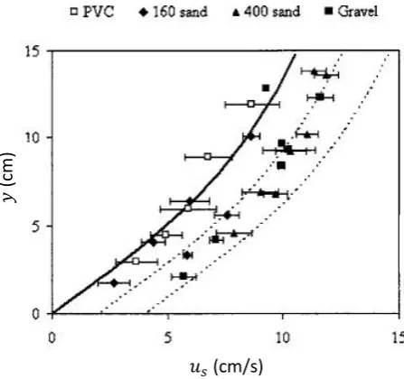
Figure 2.5: Mean velocity profiles in near-bed regions for sediment bed experiments where each point represents an average of measurements from profiles repeated for the same sediment and flow conditions. The Solid curve represents profile (2.39) with zero displacement whilst the dashed curves represent profiles with slip velocities of 2 and 4 Fries [2007]
dashed lines represent the same profile but with a horizontal displacement equal to slip flow velocitiesus = 2 andus = 4 (cm/s). The two dashed profiles fit the rough
permeable bed measurements, where as the original (solid) profile fits the smooth impermeable PVC bed measurements.
u+(y+) =
1
κln[1 + (y++ψ+)]
+ 7.8
1−exp
−y++ψ+ 11
−(Y++ψ+) 11 exp
−y++ψ+ 3
(2.39)
Where: u+is the normalised horizontal velocity,y+is the normalised elevation above
the interface,κis the Von K´arm´an constant andψ+is the normalised velocity profile
ݕ
ݑ
ݑ௦
ݔ
v Impermeable surface
Permeable bed
Figure 2.6: Pictorial representation of slip flow
The Navier-Stokes equation is a second order, nonlinear equation and in the overlying flow, in incompressible form, can be expressed as
∂u
∂t +u· ∇u=−
∇p
ρw
+ν∇2u+Fb (2.40)
where: u is the velocity vector and Fb is the net body force or gravity term in free
surface problems (which has units of acceleration).
Darcy’s law (2.41), which was empirically deduced but can also be derived from the Navier-Stokes equation through averaging over large pore volumes [O’Connor and Harvey, 2008], is a first order, linear equation. Equation (2.41) is the same as (2.26), but written in terms of pressure instead of head.
∇p
ρw
=−ν
Kv (2.41)
There are two different approaches taken by researchers when combining (2.40) and (2.41). Some, such as Basu and Khalili [1999] and Zhou and Mendoza [1993] have treated the problem as a single domain (overlying water and sediment bed as one), where as others, such as Beavers and Joseph [1967] and Ruff and Gelhar [1972], use a two domain approach.
require empirically determined interface conditions, such as the two domain problem requires, they have to contend with rapidly changing values of porosity, permeability, etc. across the sediment water interface. Consequently this region requires special treatment and correction steps [Basu and Khalili, 1999].
The two domain approach is simpler, but as stated above, relies on em-pirically derived interface properties. Generally, only the sediment portion of the problem is considered, but with the inclusion of additional force terms to Darcy’s law (2.41) [O’Connor and Harvey, 2008]. Beavers and Joseph [1967] and Ruff and Gelhar [1972] used a conceptual Brinkman boundary layer just blow the sediment water in-terface. The characteristic length scale for the Brinkman layer is √K [Beavers and Joseph, 1967] over which the additional flow resistance is generated by viscous shear stress and nonlinear form drag which are added to create the extended Darcy equation.
∇p
ρw
=−ν
Kv+νe∇
2v−√CD
Kv
2 (2.42)
Where: νe is the effective viscosity and CD is a dimensionless drag coefficient.
The third term in (2.42) represents the Brinkman term and the fourth term represents the Forchheimer term and introduces CD (the dimensionless form drag
coefficient), which is a property of the porous sediment bed [Venkataraman and Rama Mohan Rao, 1998]. Ruff and Gelhar [1972] solved for thevfield using (2.42) with an empirically derived value for CD and evaluating νe as a constant varying
with depth. This solution for v also provided an expression of the slip velocity,
us, tangential to the sediment water interface (the slip velocity is on the water side
of the interface and is not a volume average of the interstitial velocity) [O’Connor and Harvey, 2008]. Their resulting expression for slip velocity assuming a constant effective viscosity is given by
us
u∗
3
+ 3
2CDReK
us
u∗
2
= 3ReK 2CD
ν
νe
(2.43)
where: usis the slip velocity,u∗ is the bed shear velocity andReK =u∗
√
K/νis the permeability Reynolds number characterising the flow within the Brinkman layer.
Fries [2007] evaluated effective viscosity (νe) as an effective diffusion (νe≈D)
in (2.43), which can be rearranged into (2.44), allowingDto be estimated using the slip flow model.
D= 3νRe
2 K
2CDReKu3s++ 3u2s+
(2.44)
[2007] by fitting the Reichardt velocity profile (2.39) to measured velocity profiles.
2.3.3 Effective Diffusion Scaling Relationship
The complex nature of hyporheic exchange has led to the use of an effective diffu-sion coefficient which combines all the physical, biological and chemical exchange processes. It is therefore unnecessary to assume that the best means of estimating the effective diffusion coefficient is through modelling the physical processes that occur. This has led to a succession of scaling relationships being employed to relate an effective diffusion coefficient to a variety of fluid flow and sediment characteristics [O’Connor and Harvey, 2008].
The idea of a scaling relationship for hyporheic exchange was proposed by Richardson and Parr [1988]. They conducted flume experiments simulating runoff over a uniform bed (1.2m long by 25.4mm deep) of glass beads using a horizontal, 4.9 by 0.15m Plexiglas flume. Three different flow depths and four velocities were passed over five different diameters of bead, which represented fine to very course sands. The bed was saturated with tracer (fluorescein disodium salt) and the flow started. Tracer concentrations were measured at the effluent weir throughout the 30 minute experiments. This research stemmed from environmental pressures on the agricultural industry and is the start of the research into hyporheic exchange. Richardson and Parr [1988] took the Fickian model, and noted that it did not match their observed data. This led them to propose the use of a non-constant, time varying diffusion coefficient which could be used within the standard Fickian diffusion model. The time dependent diffusion coefficient (D∗) is given by
D∗ =γD (2.45)
where: γ is a time dependent variable given by
γ = 1
1− t t0
h
1−exp−tt 0
i. (2.46)
However after the initial non-Fickian phase the diffusion coefficient can be taken as constant. Richardson and Parr [1988] related their measured value for the effec-tive diffusion to the sediment properties, characterised by the permeability P´eclet number (P eK). Their scaling relationship for a time independent effective diffusion
coefficient is given by
D
D0m = 6.59×10
−5P e2
Figure 2.7: Packman and Salehin [2003] pumping model based scaling relationship showing the influence of stream velocity, permeability and porosity of the bed sedi-ments
where: P eK is the permeability P´eclet number (u∗
√
K/Dm0 ).
This relationship fits the data set used by Richardson and Parr [1988] well, however the range of sedimentary and flow conditions modelled is relatively small. This gives the relationship limited applicability. Packman and Salehin [2003] used seven different data sets to derive their own scaling relationship. They used data from Elliott and Brooks [1997b], Eylerset al.[1995], Packmanet al.[2000], Packman and MacKay [2003], Marionet al. [2002], Packman et al.[2004]1 and Nagaoka and Ohgaki [1990], which provided a much wider range of sediment and flow conditions than the single set used by Richardson and Parr [1988].
Packman and Salehin [2003] demonstrate a linear relationship between the effective diffusion coefficient and the parameter grouping Khm/θ (where K is the
permeability,hmis the amplitude of the dynamic pressure head given by (2.24) andθ
is the sediment porosity), which they demonstrate to hold for more than three orders of magnitude of bed-form driven exchange [Packman and Salehin, 2003]. However the relationship does not hold for fine sands used by Eylerset al.[1995], which has a similar effective diffusion coefficient to Elliott and Brooks [1997b] but a much lower
Khm/θ value (Figure 2.7).
Packman and Salehin [2003] also propose a linear relationship between the effective diffusion coefficient and the parameter grouping (Re dg)2 (where Reis the
1
Figure 2.8: Packman and Salehin [2003] second scaling relationship showing ex-change is proportional to the sediment size, which suggests that the permeability of the sediment bed controls exchange with both flat beds and bed-forms
stream Reynolds number (U H/ν) and dg is sediment grain diameter) and report
that it holds for almost five orders of magnitude of observed hyporheic exchange behaviour. This represents two orders of magnitude of variation in sediment grain size, almost an order of magnitude variation in stream velocity and distinctly differ-ent stream channel topographies [Packman and Salehin, 2003]. In this relationship the sediment grain size is used to represent the sediment properties such as K and
θ. However there is still deviation from this relationship within the data sets used, particularly when fine sands are used (Figure 2.8).
O’Connor and Harvey [2008] published a scaling relationship derived from a wide range of data sets that covered different sediment characteristics, flow param-eters and topographies. Like Packman and Salehin [2003], O’Connor and Harvey [2008] took data from several studies which are listed below. Table 2.1 gives the ex-perimental parameters as presented by O’Connor and Harvey [2008] and information about each paper is given in Section 2.4.
List of papers used by O’Connor and Harvey [2008] with Table 2.1 references
Richardson and Parr [1988] - a
Nagaoka and Ohgaki [1990] - b
Laiet al. [1994] - c
Marion et al.[2002] - e
Packmanet al. [2004] - f
Packmanet al. [2000] - g
Packman and MacKay [2003] - g
Ren and Packman [2004] - g
Rehget al. [2005] - g
Tonina and Buffington [2007] - h
Study dg K θ ∆ λ u∗ U H
(mm) (10−6 cm2) (cm) (cm) (cm/s) (cm/s) (cm)
Richardsona 0.1-3.0 0.17-71 0.36-0.40 0 0 0.3-1.3 3.7-22.9 0.6-1.9 Nagaokab 19.0-40.8 500-2300 0.24 0 0 1.1-4.3 8.9-42.8 3.2-7.0 Laic 0.5-3.2 2.3-19 0.36-0.38 0 0 0.2-0.6 7.4-15.4 0.5-2.0 Elliottd 0.1-0.5 0.08-1.1 0.30-0.33 1.1-2.5 9-30 1.3-2.4 8.6-13.2 3.1-6.5 Marione 0.85 5.0 0.38 0-3.5 0-120 1.7-1.8 22.0-28.0 10.9-12.3
Packmanf 4.8 150 0.38 0-3.7 0-32 1.1-3.2 9.0-36.1 11.3-20.5
Variousg 0.5 0.68-1.8 0.29-0.38 0.8-1.9 15-70 0.5-1.7 12.0-23.7 7.1-12.7 Toninah 9.8-10.8 51 0.34 3.6-12.0 515-560 3.8-5.5 28.2-46.0 3.9-10.4 Table 2.1: Summary of sediment and fluid flow conditions as presented by O’Connor and Harvey [2008]
As stated above, O’Connor and Harvey [2008] compiled data from various flume tracer studies in order to examine a wide range of fluid flow and sediment conditions and their effect on transport in permeable sediments. They evaluated a measured effective diffusion coefficient for all the studies. However the variations in the experimental setups resulted in three different methods of calculation being employed. The deciding factors on which equation to use were where the solute tracer was placed at the start of the experiment and where the sampling of solute tracer occurred. Details of the different analysis techniques are given in Section 2.4. For all studies O’Connor and Harvey [2008] used plots of either mass or concentration versus the square root of time to compute the slopes needed in the equations detailed in Section 2.4 for calculating experimentalDvalues. Not all fluid flow and sediment parameters were reported within the papers, thus O’Connor and Harvey [2008] used several different equations to estimate the missing parameters. A list is given below (the sediment parameters are discussed in Section 2.6).
• Bed shear velocity (u∗) - (2.15)
• Permeability (K) - (2.129) or (2.130)
Once O’Connor and Harvey [2008] had collated and unified all the data, Buckingham’s Π theorem was used to generate dimensionless groups of controlling variables. This process involved three stages, (i) listing the minimum number of vari-ables needed to describe hyporheic exchange, (ii) generating dimensionless groupings of the controlling variables and (iii) using the compiled hyporheic exchange data to determine a power law scaling relationship for effective diffusion [O’Connor and Harvey, 2008].
The control variables chosen represent the controlling fluid flow and sediment conditions according to both the pumping and slip flow models, given by
D=f(D0m, U, u∗, ks,
√
K, ν) (2.48)
where: Dm0 is defined by (2.2) which includesθ,ksis roughness height which includes
the variablesd90, ∆ and λ.
The seven variables in (2.48) are composed of two dimensions (L and T), which results in the possibility of five dimensionless groupings. O’Connor and Har-vey [2008] simplified the five possible groups into four groupings of dimensionless numbers known to affect hyporheic exchange.
D
D0
m
∼
U
u∗
,
u∗ks
ν
, u∗
√
K
D0
m
!
(2.49)
Where: U/u∗ = Cz is the Ch´ezy resistance coefficient, u∗ks/ν = Re∗ is the shear
Reynolds number andu∗
√
K/D0m=P eK is the permeability based P´eclet number.
Equation (2.50) is (2.49) rewritten in the form of a power law scaling relationship.
D
D0m =αC
b
zRec∗P edK (2.50)
Where: α is a dimensionless scaling constant and b, c, dare scaling exponents for the dimensionless numbers.
The next stage is to determine scaling exponents and scaling constant. This was achieved by plotting the three dimensionless numbers individually against the dimensionless diffusion coefficient (D/D0m). This revealed strong relationships be-tween the shear Reynolds number and the permeability P´eclet number. However it showed only a weak correlation betweenD/Dm0 and Cz, so the Ch´ezy resistance
Richardson Nagaoka Lai Elliott Marion Packman Various Tonina Effective Molecular
ܴ݁∗ܲ݁ ହ⁄ = 2000 (molecular diffusion → effective diffusion)
ܴ݁∗ܲ݁ ହ⁄
ܦ
ܦ′ = 5 × 10 ିସܴ݁
∗ܲ݁ ହ⁄
ܴଶ= 0.95
ܦ ܦ′
10ସ 10ଶ
10 10 10଼ 10ଵ
10ିଶ 10 10ଶ 10ସ 10 10଼
Figure 2.9: Effective diffusion scaling relationship compared against previous exper-imental data [O’Connor and Harvey, 2008]
[2008] plottedD/D0mversusRe7/4∗ P e9/4K and found it had a slope of 0.55, which was
combined with the scaling exponents to give the scaling relationship
D
D0
m
=
5×10⁻⁴Re∗P eK6/5 forRe∗P e6/5K ≥2000
1 forRe∗P e6/5K <2000
(2.51)
where the inverse of the scaling constant (5×10⁻⁴) provided a threshold value in transport conditions (Re∗P e6/5K = 2000), below which transport was governed by
molecular diffusion, resulting inD/D0m= 1.
Figure 2.9 [O’Connor and Harvey, 2008] demonstrates their scaling relation-ship and the good fit to the dataset used. All but one of the experimentalD(De in
figure) data points were above the threshold condition for molecular diffusion. The scaling relationship described by (2.51) has a slope of one and explains 95% of the variance with 95% confidence intervals of the slope between 0.93 to 1.02 [O’Connor and Harvey, 2008].
[image:45.595.135.510.109.340.2]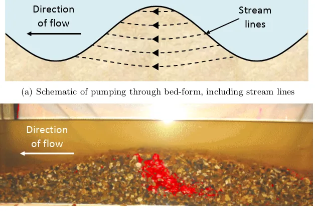
![Figure 2.4: Normalised head distribution and particle flow paths (stream lines)predicted using Elliott and Brooks [1997a] model, [Dutton, 2004]](https://thumb-us.123doks.com/thumbv2/123dok_us/9646061.466803/32.595.157.479.108.351/figure-normalised-distribution-particle-predicted-elliott-brooks-dutton.webp)
![Figure 2.9 [O’Connor and Harvey, 2008] demonstrates their scaling relation-](https://thumb-us.123doks.com/thumbv2/123dok_us/9646061.466803/45.595.135.510.109.340/figure-o-connor-harvey-demonstrates-scaling-relation.webp)