Evaluating Asset Pricing Models in a Simulated Multifactor Approach

(1)

Evaluating Asset Pricing Models in a

Simulated Multifactor Approach

Carrasco-Gutierrez, Carlos Enrique and Piazza, Wagner

Graduate School of Economics Catholic University of Brasília,

Research Department, Central Bank of Brazil

2011

(2)

Simulated Multifactor Approach

(Avaliando Modelos de Precificac¸ ˜ao de Ativos via Abordagem de Fatores Simulados)

Carlos Enrique Carrasco-Gutierrez* Wagner Piazza Gaglianone**

Abstract

In this paper a methodology to compare the performance of different stochastic discount factor (SDF) models is suggested. The starting point is the estimation of several factor models in which the choice of the fundamental factors comes from different procedures. Then, a Monte Carlo simulation is designed in order to simu-late a set of gross returns with the objective of mimicking the temporal dependency and the observed covariance across gross returns. Finally, the artificial returns are used to investigate the performance of the competing asset pricing models through the Hansen & Jagannathan (1997) distance and some goodness-of-fit statistics of the pricing error. An empirical application is provided for the U.S. stock market.

Keywords:asset pricing; stochastic discount factor; Hansen-Jagannathan distance.

JEL codes:G12; C15; C22.

Resumo

Neste artigo apresenta-se uma metodologia para comparar a performance relativa de diferentes modelos de fator estocástico de desconto (SDF - Stochastic Dis-count Factor). O ponto de partida é a estimação de modelos de fatores gerados por abordagens distintas. Em seguida, uma simulação de Monte Carlo é cons-tru´ıda para simular um conjunto de retornos (brutos) de ativos, com o intuito de

Submitted 17 February 2012. Reformulated 25 July 2012. Accepted 20 Septem-ber 2012. Published on-line 30 January 2013. The article was double blind refereed and evaluated by the editor. Supervising editor: José Fajardo. The authors thank the editor Ricardo Leal, two anonymous referees, João Victor Issler, Fabio Araujo, Caio Almeida, Carlos Eugênio, Luis Braido, Christiam Gonzales as well as participants of various confer-ences and seminars for their helpful comments and suggestions. The opinions expressed in this article are those of the authors and do not necessarily reflect those of the Banco Central do Brasil. Any remaining errors are ours.

*Graduate School of Economics, Catholic University of Bras´ılia, Bras´ılia, DF. E-mail: [email protected]

**Banco Central do Brasil, Rio de Janeiro, RJ. E-mail: wagner.gaglianone@bcb. gov.br

(3)

replicar a dependência temporal e respectivas covariâncias amostrais observadas em retornos de ativos. Por fim, os retornos artificiais são utilizados para inves-tigar a performance de modelos de precificação de ativos através da distância de Hansen & Jagannathan (1997) e de algumas estat´ısticas de teste baseadas em erros de precificação. Um exerc´ıcio emp´ırico com dados de ativos norte-americanos é apresentado para ilustrar a metodologia proposta.

Palavras-chave: precificação de ativos; fator estocástico de desconto; distância

Hansen-Jagannathan.

1. Introduction

(4)

expect that a SDF proxy based on a geometric Brownian motion assumption would perform better than an asset pricing model that does not assume this hypothesis. On the other hand, a critical issue of this procedure is that the best asset pricing model from these particular environments might not be a good model in the real world. In other words, the best estimator for each controlled framework might not necessarily exhibit the same performance for observed stock market prices of a real economy.

In this paper, we propose a methodology to compare different stochas-tic discount factor or pricing kernel proxies. Instead of generating the asset returns from a direct ad-hoc assumption about the DGP of returns, we use factor models and related market information from the real economy. The idea is to create a set of gross returns with the objective of mimicking the real world structure as closely as possible. Our starting point is the esti-mation of linear factor models (in the sense of the Arbitrage Pricing The-ory – APT of Ross, 1976), in which the choice of common factors, which usually correspond to unobserved fundamental influences on returns, come from different procedures. For example, the well-known factors of Fama & French (1993, 1996, 1998), which evidenced those asset returns of the U.S. economy, could be explained by relative factors linked to characteristics of firms. The next step is to create a framework to compare the competing as-set pricing models. In this sense, a Monte Carlo simulation is constructed to mimic, as closely as possible, the temporal dependency and the observed covariance across gross returns. Finally, the artificial returns are used to investigate the performance of the competing asset pricing models based on the performance of some statistics. In order to compare asset pricing models, several works use the HJ-distance on real data. Our strategy allows calculating the average and median of the HJ-distance across all realiza-tions of the Monte Carlo experiment, which is shown to be a useful model evaluation tool.

(5)

the paper (regarding SDF proxies comparison) are, thus, conditional on the factor models adopted to replicate returns. In other words, we implicitly assume that those models might be representative of return series, provided that the focus of the paper is grounded on SDF comparison through Monte Carlo simulation and not on factor model investigation.

Nonetheless, one advantage of this methodology is that it not only re-stricts the analysis to known factors like the three factors of Fama and French, but also allows for purely statistical procedures, such as factor anal-ysis. Moreover, the beta parameters associated with those factors are esti-mated instead of calibrated. In addition, the covariance structure across returns is conveniently taken into account in order to replicate the observed structure in the simulated setup.

To illustrate our methodology, we present a simple empirical applica-tion for the U.S. stock market, in which three SDF estimators are compared: a) the nonparametric estimator of Araujoet al.(2006); b) the Brownian mo-tion pricing model studied in Brandtet al.(2006); and c) the traditional lin-ear CAPM (see Cochrane (2001, p.152-166)). We also estimate the Hansen and Jagannathan SDF of minimum variance that will be used as a bench-mark. The common factors used in this exercise are formed by three sets: (i) factors provided by the use of the factor analysis; (ii) the well-known three-factor model of Fama & French (1993, 1996); and (iii) an extended version of the previous three-factor model of Fama and French, (Anget al., 2006, see), including momentum and short- or long-term reversal factors. In comparing asset pricing models, we use the average and median of the HJ-distances and a goodness-of-fit statistic provided by the pricing error. The result indicates that the SDF of Brandtet al.(2006) seems to be the best model, given that the Brownian motion hypothesis is able to generate SDF dynamics with adequate statistical features, which are closer to the Hansen and Jagannathan SDF.

This paper is organized as follows: Section 2 presents some stochastic discount proxies; Section 3 discusses the factor models; Section 4 shows the procedures used to replicate the gross returns and the statistical measures to evaluate the performance of the SDF estimators; Section 5 presents the empirical application for the U.S. stock market; and Section 6 concludes.

2. Stochastic Discount Factor models

(6)

(1991), associated with the stochastic discount factor (SDF), which relies on the pricing equation; pt = Et(mt+1xi,t+1), whereEt(·)denotes the

conditional expectation given the information available at timet,ptis the

asset price, mt+1 is the stochastic discount factor, and xi,t+1 is the asset

payoff of thei-th asset int+ 1. This pricing equation means that the market value today of an uncertain payoff tomorrow is represented by the payoff multiplied by the discount factor, also taking into account different states of nature by using the underlying probabilities.1 The stochastic discount factor model provides a general framework for pricing assets. As docu-mented by Cochrane (2001), asset pricing can basically be summarized by two equations:

pt = Et[mt+1xt+1] (1)

mt+1 = f(data, parameters) (2)

where the model is represented by the functionf(·), and the pricing equa-tion (1) can lead to different predicequa-tions stated in terms of returns.2

Hansen & Jagannathan (1991) propose a way to calculate the SDF and provide a lower bound on the variance of a stochastic discount factor (SDF). In fact, although the authors do not deal with a direct estimate of the SDF, they show that the mimicked discount factorM_t+1∗ has a direct relation to the minimal conditional variance portfolio. Moreover, they exploit the fact that it is always possible to project the SDF onto the space of payoffs, which makes it straightforward to express the mimicking portfolio as a function of only observable variables:

M_t+1∗ =ı′_NE_t R_t+1R′_t+1−1R_t+1 (3)

1

According to Cochrane (2001, p.68), unless markets are complete, there are an in-finite number of SDFs, but all can be decomposed as mt+1 = m∗t+1+vt+1, where

Et(vt+1Rit+1) = 0, in whichm∗t+1is called the SDF mimicking portfolio.

2_{For instance, in the Consumption-based Capital Asset Pricing Model (CCAPM)}

con-text, the first-order conditions of the consumption-based model, summarized by the well-known Euler equation:pt=Et

βu′(ct+1)

u′(ct) xt+1

. The specification ofmt+1corresponds to the intertemporal marginal rate of substitution. Hence,mt+1=f(c, β) =β

u′₍_c_t₊₁₎

u′(ct) , whereβis the discount factor for the future,ctis consumption andu(·)is a given utility

(7)

whereıN is anN ×1vector of ones, andRt+1is anN ×1vector

stack-ing all asset returns. Equation (3) delivers a nonparametric estimate of the SDF that is solely a function of asset returns. There are different estimates of the SDF derived from other hypotheses, such as the SDF derived from the hypothesis of Brownian motion pricing, the linear stochastic discount factor derived from the CAPM, and the nonparametric SDF of Araujoet al.

(2006).

i) Brownian motion pricing model

The price dynamics of a risky asset follows the basic Black & Sc-holes assumptions. Suppose that a vector of asset prices follows a geometric Brownian motion (GBM). Such hypothesis is defined by the following partial differential equation:

dP P =

Rf +µdt+ Σ12dB ₍₄₎

where, dP_P = dP1 P1 , ...,

dPN

PN

′

, µ = (µ1, ..., µN)′, Σis anN ×N

positive definite matrix, Pi is the price of the asset i, µ is the risk

premium vector, Rf is the risk-free rate, andB is a standard GBM of dimensionN. Using the Itˆo theorem, it is possible to show that:

Ri_t+∆t= P

i t+∆t

P_ti =e

(Rf_+µ

i−1₂Σi,i)∆t+

√

∆t

Σ 1 2

i

′

Zt

(5)

whereZtis a vector ofN independent variables with Gaussian

dis-tribution. Therefore, the SDF proposed by these authors is calculated as

Mt+∆t=e−(R

f₊1 2µ

′_Σ−1_µ₎_∆t₋√_∆tµ_Σ−1₂′

Zt

(6)

and the estimator of this stochastic discount factor model is given by:

c

M_t=e−(Rf+12µb

′_Σ_b−1_µ_b₎_∆t_−b_µ′_Σ_b−1₍_R

t−R¯) ₍₇₎

where,µ, Rb andΣbare estimated by:

b

µ= R¯−R

f

(8)

b

Σ = 1

∆t

1

T

X

t=1

Rt−R¯ Rt−R¯′ (9)

such that,Rt= R1t, ..., RNt

′_and_R_¯ ₌ 1 T

PT t=1Rt.

ii) Capital Asset Pricing Model – CAPM

Using the pricing equation p_t = E_t[m_t+1x_t+1], it is easy to show that this implies a single-beta representation which is also equivalent to linear models for the discount factormt+1 =a+bRw,t+1, where

R_w,t+1 is a factor relative to the market risk. Therefore, assuming the unconditional CAPM, the SDF is a linear function of market re-turns. For instance, in the U.S. economy, in order to implement the CAPM, for practical purposes, it is commonly assumed that the re-turn on the value-weighted portfolio of all stocks listed on the NYSE, AMEX, and NASDAQ is a reasonable proxy for the return on the market portfolio of all assets of the U.S. economy.

iiii) Araujoet al.(2006)

An estimator for the stochastic discount factor within a panel data context is proposed by Araujoet al.(2006). This estimator assumes that, for every asset i∈ {1, ..., N}, the vector process{ln(M_tR_t)}

is covariance stationary with finite first and second moments. In ad-dition, under no arbitrage and some mild additional conditions, they show that a consistent estimator for a positive SDFM_tis given by:

c Mt=

¯

RG_t

1 T

PT

t=1R¯AtR¯Gt

!

(10)

whereR¯A_t = _N1 PN_i=1Ri,tandR¯Gt = ΠNi=1R

−N1

i,t are respectively the

cross-sectional arithmetic and geometric mean of all gross returns. Therefore, this nonparametric estimator depends exclusively on ap-propriate means of asset returns that can easily be implemented.3

3

(9)

3. Multifactor Pricing Models

A benchmark for the development of asset pricing models is the work of Sharpe (1964), which proposed the well-known Capital Asset Pricing Model (CAPM). The CAPM approach is based on a single factor to explain different return series and, despite its simplicity, quite often does not exhibit a good fit to real data. In this sense, Ross (1976) proposed a multifactor approach based on “no arbitrage” assumptions to explain return series, re-sulting in the so-called APT (Arbitrage Pricing Theory) model. Afterward, Fama & French (1993) suggested the 3-factor model, based on market and firms characteristics, with the aim of improving the fit to return data and capture market anomalies. Based on the “momentum” factor of Jegadeesh & Titman (1993), the 4-factor model is later proposed by Carhart (1997).

More recently, Grinblatt & Titman (2002) divides the factor model literature into three main categories: (i) factors derived from macroeco-nomic variables (e.g., CAPM, ICAPM - Intertemporal Capital Asset Pric-ing Model (see Cochrane (2001, p.166) for further details)); (ii) factors based on firm attributes; and (iii) factors based on statistical procedures. In this work, we ground the analysis on categories (ii) and (iii) by using the Fama-French (standard and extended) factors and principal component-based factors to replicate return series. Nonetheless, it is worth mentioning that different approaches could also be employed to generate artificial re-turns from multifactor models (see Campbellet al.(1997, p.219) for a good survey).

We start investigating the APT model of Ross (1976) in order to use a multifactor pricing model to reproduce artificial asset returns. Con-sider a K-factor model from a set of observed gross returns

Rt= (R1t, R2t, ..., RN t)′,

Rit=ai+ K

X

k=1

Xt,kβi,k+εit, t= 1,2, ..., T (11)

in which K is the total number of common components or factors Xt,k.

(10)

Factor models summarize the systematic variation of theN elements of the vectorRtusing a reduced number ofK factors. The expected return-beta

expression of a factor pricing model is:

E(Ri) =γ+ K

X

k=1

βi,kλk+εi, i= 1,2, ..., N (12)

whereλ_kis interpreted as the price of thek-th risk factor.

Fama and French constructed factors and developed the pricing model that combined these factors to explain the average of stock returns. They evidenced that some factors can (relatively well) explain the average of stock returns.4 They showed that, besides the market risk, there are other important related factors, such as size, book-to-market ratio, momentum and leverage, among others, that help explain the average return in the stock market. The authors mentioned that these factors are indeed related to economic fundamentals and these additional factors might (quite well) help to understand the dynamics of the average return. This evidence has been demonstrated in subsequent works and for different stock markets (see Gaunt (2004) and Griffin (2002) for a good review).5 The main three fac-tors, described below, are the SMB, HML and RM.

(i) The SMB (Small Minus Big) factor is constructed to measure the size premium. In fact, it is designed to track the additional return that investors have historically received by investing in stocks of compa-nies with relatively small market capitalization. A positive SMB in a given month indicates that small cap stocks have outperformed the large cap stocks in that month. On the other hand, a negative SMB suggests that large caps have outperformed.

(ii) The HML (High Minus Low) factor is constructed to measure the

premium-valueprovided to investors for investing in companies with

high book-to-market values. A positive HML in a given month sug-gests that “value stocks” have outperformed “growth stocks” in that

4_{Indeed, all the results of this paper confirm that the model of Fama and French better}

explains the average return of stocks in comparison to the CAPM model.

5_{However, this finding is not a consensus in the literature. For instance, Daniel &}

(11)

month, whereas a negative HML indicates the opposite.6

(iii) The Market factorRM = R_M −R_f is the market excess return in comparison to the risk-free rate. For example, in the U.S. economy, the RM can be proxied by the value-weighted portfolio of all stocks listed on the New York Stock Exchange (NYSE), the American Stock Exchange (AMEX), and NASDAQ stocks (from CRSP data) minus the one-month Treasury Bill rate.

Considering these three factors, the factor model for expected returns is given by:

E(Rit)−Rf t = βim[E(RM t)−Rf t] +βisE(SM Bt) (13)

+ βihE(HM Lt), i∈ {1, ..., N}

where the betasβim,βisandβihare slopes in the multiple regression (13).

Hence, one implication of the expected return equation of the three-factor model is that the intercept in the time-series regression (14) is zero for all assetsi:

Rit−Rf t=βimRMt+βisSM Bt+βihHM Lt+εit (14)

whereRM_t = (R_{M t}−R_{f t}). Using this criterion, Fama & French (1993, 1996) find that the model captures much of the variation in the average re-turn for portfolios formed on size, book-to-market ratio and other price ra-tios. The Fama and French approach is (in fact) a multifactor model that can be seen as an expected beta7 representation of linear factor pricing models of the form:

E(Ri) =γ+βimλm+βisλs+βihλh+ǫi, i∈ {1, ..., N} (15)

6

Notice that, in respect to SMB, small companies logically are expected to be more sensitive to many risk factors, as a result of their relatively undiversified nature and also their reduced ability to absorb negative financial shocks. On the other hand, the HML factor suggests higher risk exposure for typical value stocks in comparison to growth stocks. See Perez-Quiros & Timmermann (2000), Cochrane (2001, p.441) and Marinelli (2011) for possible interpretation of such factors.

7_{The main objective of the beta model is to explain the variation in terms of average}

(12)

By running this cross sectional regression of average returns on betas, one can estimate the parameters (γ, λm,λs, λh). Notice that γ is the

in-tercept andλm,λsand λh are the slope in this cross-sectional relation. In

addition, the βim,βisandβihare the unconditional sensitivities of thei-th

asset to the factors.8 Moreover,β_ij, for somej ∈ {m, s, h}, can be inter-preted as the amount of risk exposure of asset ito factorj, andλj as the

price of such risk exposure.

On the other hand, one can use factors different from the Fama-French approach to help explaining the variation of cross-section assets. An inter-esting example is the statistical technique known as factor analysis, which has been used to estimate factors from a huge quantity of asset returns. Factor analysis explains the covariance relationships among a number of observed variables in terms of a much smaller number of unobserved vari-ables, termed factors, which reduces the dimensionality of the problem. In other words, this approach allows one to identify a small set of orthogonal unobservable factors by summarizing all the information contained in the original dataset (see Tucker & MacCallum (1993) and Johnson & Wichern (1992) for further details). The factor analysis technique applied to gross return seriesRitinvolves the following model:

R_it=µ_i+

J

X

j=1

L_i,jF_j,t+v_it (16)

whereJ is the number of factors adopted,µiis the unconditional mean of

the gross returns, Li,j represents the factor loading (i.e., the contribution

of each return to the variation of each factor), Fj,t is the j-th factor and

vit is an error term with zero mean and finite variance. Therefore, by

us-ing principal component analysis to estimate, for example, three factors, provided that the first factor alone F1,t accounts for xpercent of the total

variance, whereas the second (F2,t) and the third (F3,t) ones account fory

andzpercent of the total variance, respectively, we have thatx > y > z.

4. Replicating Return Time Series

Now we construct hypothetical returns using the multifactor pricing models. We first estimate the beta parameters from a linear factor model.

8

(13)

Then, we replicate the returns by creating artificial series which mimic the real world ones. Finally, based on the artificial returns created through a Monte Carlo simulation, we evaluate the SDF candidates within this con-trolled setup.

A Controlled Environment to Simulate Portfolios

Since the objective of this paper is to provide a controlled setup to eval-uate SDF estimators, we now present a simple methodology to replicate return series based on factor models. Given that a linear factor model ap-proach is adopted to mimick the real world returns, we now focus on the methodology to replicate a vector of returns from a set ofXt,kfactors.

The followingK-factor model is given by:

R_it=a_i+

K

X

k=1

X_t,kβ_i,k+ε_it (17)

Following the approach of Ren and Shimotsu (2006), we firstly esti-mate the beta parameters and collect the residuals εit in order to compute

the respective sample covariances (here summarized by the covariance ma-trix Ω). This covariance matrix is used in the simulation exercise as an additional information to theK factors. In this way, the simulated returns can account for both the factors and the model-based residual covariance structure. Second, we run the following cross-sectional regression (i.e., a standard one-dimension regression along i ∈ {1, ..., N}, which refers to the assets index):

E(Ri) =α+ K

X

k=1

(E(Xt,k) +ηk)βi,k+ui (18)

which gives the estimates of the risk-free rate αb and the factor-mean ad-justed risk prices ηb_k based on: (i)βb_i,k estimated in (17); (ii) the sample

proxies forE(Ri)andE(Xt,k), that is,E(Ri)≡ _T1 T

P

t=1

Ritfori= 1, ..., N

and E(X_t,k) ≡ _T1

T

P

t=1

X_t,k fork = 1, ..., K; and (iii) the residual of the

regressionui. After that, we considered random factors based on normal

(14)

their sample variance.9 10 Finally, we create artificial return series Reit,

based on the following equation:

e

Rit=αb+ K

X

k=1

(Xt,k+ηbk)βbi,k+εeit (19)

in whichXt,kare the adopted factors,εeit= Ω1/2ǫitandǫitare drawn from

independent standard normal distributions. Notice that, since E(ǫitǫ′it) =

I, it follows by construction that E(ε_eiteε′it) = Ω. Considering the error

structure in the multifactor model, the set of asset spans (at least, reason-ably) the return space.

The objective here is to make the mean and variance of simulated re-turns as close as possible to the assumed factor models. The next step is to estimate the SDFs based on the artificial return seriesReitand further

evaluate (to compare the competing SDF estimators) them through Hansen-Jagannathan distance and a goodness-of-fit statistic, which are discused in the next section. It is worth mentioning that we repeat the previous steps for an amount ofnreplications in order to complete the Monte Carlo sim-ulation. For each replication, we split the set of N generated assets into two groups (with the same number of time series observations within each group). Firstly, consider an amount ofN < N˜ assets to estimate the SDF candidates (henceforth, this first group of assets will be denominated

in-sample). Based on the estimated SDF proxies and using the remaining

(N −N˜)assets, used to generate theout-of-sampleexercise (based on the approach of Fama & MacBeth (1973)), we compute the goodness-of-fit statistic in order to compare the performance of each SDF candidate and the Hansen-Jagannathan distance. In other words, we want to know how well the proxies are carried on when new information is considered.

Pricing Error of stochastic discount factor models

i) Hansen and Jagannathan distance

In the asset pricing literature, some measures are suggested to com-pare competing asset pricing models. The most famous measure is

9

In order to consider more volatile factors we use (instead of the sample variance) an estimative of the interpercentil distance among theNreal assets.

10

(15)

the Hansen and Jagannathan distance, which is employed in this pa-per to test for model misspecification and compare the pa-performance of different asset pricing models.

The Hansen & Jagannathan (1997) measure is a summary of the mean pricing errors across a group of assets. As shown by Hansen and Jagannathan, the HJ-distance δ = minm∈Mky−mk, defined

in the L2 space, is the distance of the SDF model y to a family of SDFs,m∈ M, that correctly price the assets. In other interpretation, Hansen and Jagannathan show that the HJ-distance is the pricing er-ror for the portfolio that is most mispriced by the underlying model. The pricing error can be written by α_t = E_t(m_t+1R_i,t+1) − 1. Notice, in particular, that αt depends on the considered SDF, and

the SDF is not unique (unless markets are complete). Thus, differ-ent SDF proxies can produce similar HJ measures. In this sense, even though the investigated SDF models are misspecified, in prac-tical terms, we are interested in those models with the lowest HJ-distance.11 In the special case of linear factor pricing models, the HJ-distance takes the following form (see Ren & Shimotsu (2006) for details):

HJ(δ) =E(wt(δ))′G−1E(wt(δ))1/2 (20)

wherewt(δ) =RtXt′δ−ıN;G=E(RtR′t)andXtis a factor vector

including a column of 1’s.

ii) Goodness-of-fit statisticWe also use a pricing error statistic to

com-pare stochastic discount factor models, which is derived from the following equations, as mentioned by Cochrane (2001, p.81).

α_t=E_t[m_t+1R_i,t+1]−1; i= 1, ..., N (21)

11

(16)

Note that (theoretically) the pricing error should be null (i.e.,αt= 0

for∀t). However, in practice, due to finite sample data and possible model (mis)specification, in general, we have thatαt 6= 0.

Nonethe-less, the statistical significance of αt can be used as a model

spec-ification test. In the language of excess returns, we investigate the pricing errors through the distance between actual and predicted re-turns. LetERe_i,t ≡ ER_i,t−Rf_texpress the expected excess returns. For notation simplification we denote ERe_i,t simply by

E(Re). From Cochrane (2001, p.96) we have thatE(mRe) = 0. Now, recall thatE(mRe) = E(m)E(Re) +cov(m, Re). Thus, it follows that:

E(Re) =−cov(m, R

e₎

E(m) (22)

The pricing error based on excess returns (now labelled asP r) can be defined by

P r = E(m)

E(Re)−

−cov(m, R

e₎

E(m)

(23)

= 1

Rf ∗(actual mean excess return – predicted mean excess return)

whereE(Re)is computed from actual mean excess return (i.e., estimated through the sample average of Re_i,t along the time dimension) and

−cov(m,R_E(m)e) is the mean excess return predicted by equation (22), in which

cov(m, Re)is estimated via the sample covariance betweenmandRe. Let

c

M_tsbe the SDF proxy provided by the modelsin a familySof asset pricing models. Therefore, based on equation (23), the suggested (finite sample) goodness-of-fit statistic is based on the sum of squared pricing errorsP r

(see (Cochrane, 2001, p.81)) for further details):

b p₁_s = 1

N

X

i=1

1

T

X

t=1

(Re_i,t) +cov(Mc

s t, Rei,t) 1

T

PT t=1Mcts

!2

, f or s∈S (24)

(17)

to generate theout-of-sample returns in order to compute the Hansen and Jagannathan distance. That is, we want to know how well the SDF proxies are carried on when new information is considered.

5. Empirical Application

In order to present our methodology, we investigate the performance of three different SDF estimators described in section 3, which are the Brow-nian motion pricing, the linear stochastic discount factor of the CAPM and the SDF proposed by Araujoet al. (2006). We also estimate the SDF of Hansen and Jagannathan as a benchmark.

5.1 Data

The U.S. portfolios dataset was extracted from the Kenneth R. French website12 and the asset return of the Standard & Poor’s 500 stock-market was obtained from the Yahoo Finance web site. The U.S. Treasury Bill return is used as a measure of the risk-free asset. The primitive portfolios used in competing SDFs models are described as follows:

i) 25 portfolios which contain value-weighted returns for the intersec-tions of 5 ME portfolios and 5 BE/ME portfolios.13

ii) 48 industrial portfolios which contain value-weighted returns for 48 industry portfolios.

iii) 96 portfolios which contain value-weighted returns for the intersec-tions of 10 ME portfolios and 10 BE/ME portfolios.

For a robustness check, we consider three distinct sample periods:

i) 280 observations corresponding to the period of February 1987 to July 2010.

ii) 350 observations corresponding to the period of March 1982 to July 2010.

iii) 500 observations corresponding to the period of May 1969 to July 2010.

12_{More information about data can be found in}_{http://mba.tuck.dartmouth.edu/}

pages/faculty/ken.french/data_library.html. For other economies, the factors can be constructed as showed in Fama & French (1992, 1993).

13

(18)

In order to construct the set of factors based on Factor Analysis (FA) we use monthly S&P500 stock returns14covering the period from February 1987 to July 2010. Moreover, we only consider companies for which data from S&P500 are available throughout the whole considered period, which reduces the cross-section sample fromN = 500toN = 263. This data reduction comes from the fact that the S&P500 dataset is not balanced (i.e., it is not based on a fixed set of companies throughout time, since the firms that compound the index are revised in a frequent basis15), which makes it difficult to deal with largeN and T dimensions, such thatN represents a fixed set of companies for a long span of time periods T. Thus, although the aggregate S&P500 index is available much far before 1987, from the set ofN = 500firms, which compound the index, less than 150 (surviving companies) would be available to construct factors in the case ofT = 350. Since the larger is the set of considered companies the better is the motiva-tion to employ the principal component technique, we have decided to only investigateT = 280in this case.

5.2 Factors

We use the three factors construted by Fama and French, thus the first set of factors is: (i)Xt={Rex_{M t};SM Bt;HM Lt}. Provided that the

three-factor model of Fama & French (1993, 1996) is not an unanimous approach in the literature, we also investigate an extend version by including momen-tum,M om_t, short-term reversalST Rev_tand long-term reversalLT Rev_t

factors, in order to increase the fit of the factor model to the actual data (Farnsworth et al., 2002, see). For example, the momentum factor is de-fined as the average return on the two high prior return portfolios minus the average return on the two low prior return portfolios, and the short-term and long-term reversal factors are defined as the average return on the two low prior return portfolios minus the average return on the two high prior return

14

The S&P500 index is based on the stock prices of 500 companies (mostly from the United States) selected by a committee, in order to be representative of the industries in the U.S. economy. Nonetheless, the index nowadays includes a handful set of non-U.S. companies (15 as of May 8, 2012). This group includes both formerly U.S. companies that have reincorporated outside the United States, as well as firms that have never been incorporated in the U.S.

15_{In order to keep the S&P 500 index reflective of American stocks, the constituent}

(19)

portfolios. In addition, the (i) short-term reversal factor, (ii) the momentum factor and (iii) the long-term reversal factor are based on previous (i)t−1; (ii)t−2tot−12and (iii)t−13tot−60months, respectively.16 This way, the second set of factors is given by (ii)Xt={R_{M t}ex;SM Bt;HM Lt;

M om_t;ST Rev_t;LT Rev_t}. In addition to the Fama and French factors we also construct a new set of factors, based on purely statistical grounds, using assets from the S&P500 stock market.

We use the factor analysis technique17 to construct a set ofK factors. In this setup, we study a set of factors generated by the factor analysis

K = 3, (iii) Xt = {F1,t;F2,t;F3,t}. In summary, we study three set of

factors: (i) The Fama and French factors Xt = {R_{M t}ex;SM Bt;HM Lt};

(ii) The extendend Fama and French setupX_t = {Rex_{M t};SM B_t;HM L_t;

M omt;ST Revt;LT Revt}; and (iii) The Factor Analysis set of factors

Xt ={F1,t;F2,t;F3,t}.

5.3 Results

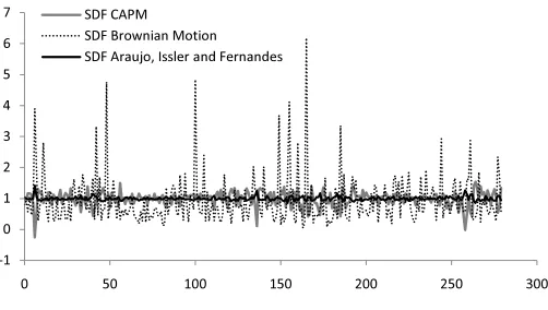
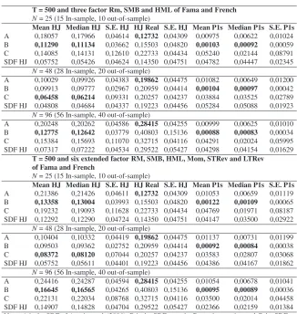
Based on a given set of observed gross returns, we construct a Monte Carlo simulation in order to replicate the observed returns and further eval-uate the competing SDF estimators. Then, we estimate the stochastic dis-count factors based on the returns generated from the factor models, and repeat the mentioned procedure for an amount ofn= 5,000 replications. Some descriptive statistics of the generated SDFs are presented in Ap-pendix (table A.1). Finally, the evaluation of the SDF proxies is conducted and the simulation results are summarized by goodness-of-fit statistic and the HJ-distance, which are averaged across all replications. We denote the SDF proxies, estimated in each replication, as modelsA,BandCto Araujo

et al.(2006), Brownian Motion and CAPM, respectively. In addition, the

stochastic discount factor implied by the Hansen & Jagannathan (1991) setup is estimated as a benchmark, denoted bySDF HJ. In Figure 1, the estimates of the SDF proxies are shown for one replication of the Monte Carlo simulation, withN = 96 and T = 280. A simple graphical inves-tigation reveals that the Brandtet al.(2006), and the Araujo et al.(2006) proxies are, respectively, the most and less volatile ones; which is a result confirmed by the descriptive statistics of Table A.1 (in Appendix).

16

See more details in the Kenneth French web sitehttp://mba.tuck.dartmouth. edu/pages/faculty/ken.french/data_library.html

17

(20)

ϰ ϱ ϲ

ϳ ^&WD

^&ƌŽǁŶŝĂŶDŽƚŝŽŶ ^&ƌĂƵũŽ͕/ƐƐůĞƌĂŶĚ&ĞƌŶĂŶĚĞƐ

Ͳϭ Ϭ ϭ Ϯ ϯ

[image:20.595.95.346.55.197.2]

Ϭ ϱϬ ϭϬϬ ϭϱϬ ϮϬϬ ϮϱϬ ϯϬϬ

Figure 1

SDF models withN= 96andT = 280

Figure 1 shows one replication out of the total amount of 5,000 repli-cations. We adoptN = 96(56 in-sample and 40 out-of-sample) assets and three factors obtained from the factor analysis.

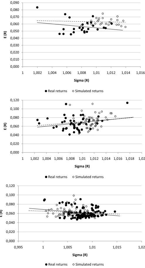
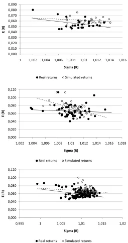
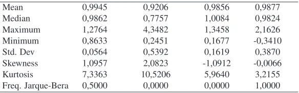
We show in Figure 2 and Figure 3, for illustrative purposes, in a “mean

versus variance” plot, the real returns and one replication of the

(21)

Ϭ͕ϬϬϬ Ϭ͕ϬϭϬ Ϭ͕ϬϮϬ Ϭ͕ϬϯϬ Ϭ͕ϬϰϬ Ϭ͕ϬϱϬ Ϭ͕ϬϲϬ Ϭ͕ϬϳϬ Ϭ͕ϬϴϬ Ϭ͕ϬϵϬ

ϭ ϭ͕ϬϬϮ ϭ͕ϬϬϰ ϭ͕ϬϬϲ ϭ͕ϬϬϴ ϭ͕Ϭϭ ϭ͕ϬϭϮ ϭ͕Ϭϭϰ ϭ͕Ϭϭϲ

;

Z

Ϳ

^ŝŐŵĂ;ZͿ

ZĞĂůƌĞƚƵƌŶƐ ^ŝŵƵůĂƚĞĚƌĞƚƵƌŶƐ

Ϭ͕ϬϴϬ Ϭ͕ϭϬϬ Ϭ͕ϭϮϬ

Ϭ͕ϬϬϬ Ϭ͕ϬϮϬ Ϭ͕ϬϰϬ Ϭ͕ϬϲϬ

ϭ ϭ͕ϬϬϮ ϭ͕ϬϬϰ ϭ͕ϬϬϲ ϭ͕ϬϬϴ ϭ͕Ϭϭ ϭ͕ϬϭϮ ϭ͕Ϭϭϰ ϭ͕Ϭϭϲ ϭ͕Ϭϭϴ ϭ͕ϬϮ

;

Z

Ϳ

^ŝŐŵĂ;ZͿ

Ϭ͕ϬϬϬ Ϭ͕ϬϮϬ Ϭ͕ϬϰϬ Ϭ͕ϬϲϬ Ϭ͕ϬϴϬ Ϭ͕ϭϬϬ Ϭ͕ϭϮϬ

Ϭ͕ϵϵϱ ϭ ϭ͕ϬϬϱ ϭ͕Ϭϭ ϭ͕Ϭϭϱ ϭ͕ϬϮ

;

Z

Ϳ

^ŝŐŵĂ;ZͿ

[image:21.595.97.344.57.512.2]

Figure 2

(22)

Ϭ͕ϬϬϬ Ϭ͕ϬϭϬ Ϭ͕ϬϮϬ Ϭ͕ϬϯϬ Ϭ͕ϬϰϬ Ϭ͕ϬϱϬ Ϭ͕ϬϲϬ Ϭ͕ϬϳϬ Ϭ͕ϬϴϬ Ϭ͕ϬϵϬ

ϭ ϭ͕ϬϬϮ ϭ͕ϬϬϰ ϭ͕ϬϬϲ ϭ͕ϬϬϴ ϭ͕Ϭϭ ϭ͕ϬϭϮ ϭ͕Ϭϭϰ ϭ͕Ϭϭϲ

;

Z

Ϳ

^ŝŐŵĂ;ZͿ

Ϭ͕ϬϲϬ Ϭ͕ϬϴϬ Ϭ͕ϭϬϬ Ϭ͕ϭϮϬ

;

Z

Ϳ

Ϭ͕ϬϬϬ Ϭ͕ϬϮϬ Ϭ͕ϬϰϬ

ϭ͕ϬϬϮ ϭ͕ϬϬϰ ϭ͕ϬϬϲ ϭ͕ϬϬϴ ϭ͕Ϭϭ ϭ͕ϬϭϮ ϭ͕Ϭϭϰ ϭ͕Ϭϭϲ ϭ͕Ϭϭϴ

^ŝŐŵĂ;ZͿ

Ϭ͕ϬϬϬ Ϭ͕ϬϮϬ Ϭ͕ϬϰϬ Ϭ͕ϬϲϬ Ϭ͕ϬϴϬ Ϭ͕ϭϬϬ Ϭ͕ϭϮϬ

Ϭ͕ϵϵϱ ϭ ϭ͕ϬϬϱ ϭ͕Ϭϭ ϭ͕Ϭϭϱ ϭ͕ϬϮ

;

Z

Ϳ

^ŝŐŵĂ;ZͿ

[image:22.595.94.349.54.538.2]

Figure 3

(23)

[image:23.595.55.384.80.460.2]

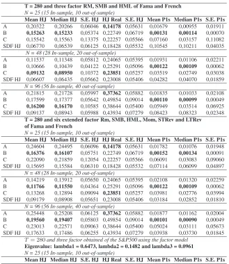
Table 1

Monte Carlo simulation results forT = 280

T = 280 and three factor RM, SMB and HML of Fama and French N = 25 (15 In-sample, 10 out-of-sample)

Mean HJ Median HJ S.E. HJ HJ Real S.E. HJ Mean P1s Median P1s S.E. P1s

A 0,20322 0,20266 0,06046 0,14178 0,05631 0,01679 0,00955 0,01911

B 0,15263 0,15233 0,05374 0,22749 0,06719 0,00131 0,00114 0,00070

C 0,15542 0,15563 0,13375 0,22257 0,05566 0,07160 0,03157 0,11082

SDF HJ 0,06770 0,06539 0,06125 0,18428 0,05532 0,10545 0,10211 0,04035

N = 48 (28 In-sample, 20 out-of-sample)

A 0,11537 0,11348 0,05812 0,24065 0,05395 0,01931 0,01106 0,02211

B 0,10666 0,10439 0,04122 0,25291 0,05096 0,00122 0,00109 0,00062

C 0,09132 0,08950 0,10372 0,23851 0,05257 0,03519 0,02749 0,03038

SDF HJ 0,06607 0,06435 0,05662 0,23008 0,05406 0,04282 0,04070 0,01859

A 0,21815 0,21728 0,05997 0,37362 0,05882 0,01835 0,01033 0,02108

B 0,17599 0,17377 0,05642 0,49854 0,09014 0,00110 0,00099 0,00049

C 0,16200 0,16170 0,10585 0,38644 0,05400 0,05949 0,03514 0,06925

SDF HJ 0,09137 0,08943 0,05988 0,43934 0,07279 0,08423 0,08323 0,02348

T = 280 and six extended factor Rm, SMB, HML, Mom, STRev and LTRev of Fama and French

A 0,24604 0,24495 0,06096 0,14178 0,05631 0,01782 0,01076 0,01948

B 0,16376 0,16107 0,05751 0,22749 0,06719 0,00152 0,00134 0,00091

C 0,22090 0,21859 0,12054 0,22257 0,05566 0,06091 0,03083 0,09060

SDF HJ 0,15695 0,15584 0,06310 0,18428 0,05532 0,07114 0,06099 0,04897

A 0,14219 0,13912 0,05650 0,24065 0,05395 0,02108 0,01320 0,02259

B 0,11766 0,11550 0,04364 0,25291 0,05096 0,00122 0,00109 0,00062

C 0,13268 0,12894 0,09094 0,23851 0,05257 0,03981 0,02776 0,03994

SDF HJ 0,09179 0,08908 0,05651 0,23008 0,05406 0,03184 0,02852 0,01810

A 0,25448 0,25208 0,06125 0,37362 0,05882 0,01877 0,01162 0,02004

B 0,19560 0,19407 0,05803 0,49854 0,09014 0,00101 0,00090 0,00049

C 0,23013 0,22571 0,09063 0,38644 0,05400 0,05024 0,03111 0,05673

SDF HJ 0,17633 0,17486 0,06255 0,43934 0,07279 0,03938 0,03730 0,01845

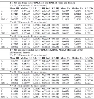
T = 280and three factor obtained of the S&P500 using the factor model Eigenvalue: lambda1 = 0.6473, lambda2 = 0.1482 and lambda3 = 0.0961 N = 25 (15 In-sample, 10 out-of-sample)

A 0,09758 0,09317 0,06029 0,14178 0,05631 0,02719 0,01716 0,03041

B 0,08595 0,08511 0,02903 0,22749 0,06719 0,00044 0,00038 0,00029

C 0,11200 0,09633 0,08156 0,22257 0,05566 0,05503 0,03040 0,07884

SDF HJ 0,03172 0,02796 0,06140 0,18428 0,05532 0,05253 0,04769 0,02887

A 0,10767 0,10343 0,05922 0,24065 0,05395 0,03785 0,02924 0,03378

B 0,09722 0,09615 0,03715 0,25291 0,05096 0,00129 0,00118 0,00057

C 0,12123 0,11018 0,07172 0,23851 0,05257 0,06573 0,04574 0,06613

SDF HJ 0,03129 0,02901 0,05775 0,23008 0,05406 0,05209 0,05027 0,02020

A 0,14125 0,13917 0,05918 0,37362 0,05882 0,03074 0,02020 0,03127

B 0,13851 0,13744 0,05076 0,49854 0,09014 0,00085 0,00078 0,00037

C 0,16247 0,14041 0,07646 0,38644 0,05400 0,05587 0,03158 0,06977

(24)

[image:24.595.56.382.79.423.2]

Table 2

T = 350 and three factor RM, SMB and HML of Fama and French

N= 25 (15 In-sample, 10 out-of-sample)

A 0,23286 0,23146 0,05425 0,14267 0,04966 0,01535 0,00938 0,01613

B 0,17224 0,17237 0,05039 0,23868 0,07222 0,00155 0,00131 0,00099

C 0,18004 0,18316 0,13294 0,24453 0,04906 0,07968 0,03418 0,12634

SDF HJ 0,07657 0,07475 0,05466 0,18899 0,05060 0,13368 0,13090 0,04479

A 0,13860 0,13758 0,05182 0,21400 0,05124 0,01898 0,01158 0,01985

B 0,11845 0,11604 0,04229 0,22224 0,04719 0,00115 0,00103 0,00055

C 0,10382 0,10303 0,11297 0,21491 0,04884 0,05253 0,04754 0,03790

SDF HJ 0,08122 0,07960 0,05102 0,19248 0,04931 0,06186 0,05944 0,02211

A 0,23969 0,23845 0,05392 0,32353 0,05484 0,01630 0,00983 0,01775

B 0,18914 0,18713 0,05357 0,53998 0,18199 0,00115 0,00101 0,00059

C 0,17707 0,18152 0,11039 0,37562 0,04943 0,06561 0,03737 0,07805

SDF HJ 0,09292 0,09136 0,05391 0,40840 0,06022 0,10352 0,10261 0,02463

T = 350 and six extended factor RM, SMB, HML, Mom, STRev and LTRev of Fama and French

A 0,26776 0,26787 0,05449 0,14267 0,04966 0,01655 0,01032 0,01688

B 0,16417 0,16161 0,05212 0,23868 0,07222 0,00145 0,00113 0,00119

C 0,23406 0,23403 0,12390 0,24453 0,04906 0,07256 0,03476 0,11636

SDF HJ 0,14746 0,14606 0,05651 0,18899 0,05060 0,09304 0,08354 0,05372

A 0,13698 0,13521 0,05138 0,21400 0,05124 0,02037 0,01327 0,02073

B 0,11827 0,11623 0,04054 0,22224 0,04719 0,00111 0,00099 0,00055

C 0,11786 0,11499 0,08435 0,21491 0,04884 0,05229 0,04239 0,04330

SDF HJ 0,08261 0,08097 0,05116 0,19248 0,04931 0,05656 0,05387 0,02311

A 0,26968 0,26850 0,05393 0,32353 0,05484 0,01703 0,01070 0,01763

B 0,19361 0,19239 0,05204 0,53998 0,18199 0,00076 0,00068 0,00039

C 0,24024 0,23875 0,09201 0,37562 0,04943 0,05351 0,03301 0,06269

SDF HJ 0,16910 0,16821 0,05573 0,40840 0,06022 0,04592 0,04362 0,01937

Note: A is the SDF of Araujoet al.(2006); B is the SDF over the Brownian motion and C the SDF

(25)

[image:25.595.55.381.78.422.2]

Table 3

T = 500 and three factor Rm, SMB and HML of Fama and French

A 0,18057 0,17966 0,04614 0,12732 0,04309 0,00975 0,00622 0,01024

B 0,11290 0,11134 0,03662 0,15503 0,04820 0,00103 0,00092 0,00059

C 0,14085 0,14131 0,12610 0,22733 0,04434 0,05240 0,02144 0,08791

SDF HJ 0,05752 0,05426 0,04624 0,14350 0,04751 0,04782 0,04447 0,02345

A 0,10029 0,09926 0,04383 0,19862 0,04475 0,01082 0,00649 0,01200

B 0,09913 0,09777 0,02967 0,20959 0,04414 0,00104 0,00097 0,00042

C 0,06458 0,06214 0,09331 0,20257 0,04237 0,03884 0,03525 0,02789

SDF HJ 0,04808 0,04684 0,04337 0,19223 0,04456 0,05284 0,05088 0,01923

A 0,20248 0,20262 0,04586 0,28415 0,04255 0,00999 0,00625 0,01010

B 0,12775 0,12642 0,03779 0,40803 0,15136 0,00088 0,00083 0,00034

C 0,15384 0,15693 0,11070 0,32715 0,04116 0,04291 0,02024 0,05995

SDF HJ 0,07317 0,07222 0,04534 0,29522 0,05427 0,04298 0,04154 0,01629

T = 500 and six extended factor RM, SMB, HML, Mom, STRev and LTRev of Fama and French

A 0,21386 0,21426 0,04611 0,12732 0,04309 0,01053 0,00659 0,01119

B 0,13358 0,13004 0,03993 0,15503 0,04820 0,00122 0,00109 0,00065

C 0,19232 0,19093 0,11628 0,22733 0,04434 0,04769 0,01971 0,08187

SDF HJ 0,12292 0,12290 0,04724 0,14350 0,04751 0,04147 0,03500 0,02922

A 0,10404 0,10332 0,04419 0,19862 0,04475 0,01137 0,00731 0,01199

B 0,09503 0,09362 0,02752 0,20959 0,04414 0,00092 0,00084 0,00038

C 0,08372 0,08120 0,07044 0,20257 0,04237 0,03583 0,02807 0,03068

SDF HJ 0,05752 0,05611 0,04401 0,19223 0,04456 0,04386 0,04167 0,01862

A 0,24416 0,24287 0,04594 0,28415 0,04255 0,01054 0,00678 0,01041

B 0,16645 0,16565 0,04265 0,40803 0,15136 0,00095 0,00089 0,00036

C 0,22131 0,22034 0,08768 0,32715 0,04116 0,03500 0,02014 0,04458

SDF HJ 0,14907 0,14828 0,04704 0,29522 0,05427 0,02366 0,02159 0,01384

Note: A is the SDF of Araujoet al.(2006); B is the SDF over the Brownian motion and C the SDF

provided by the CAPM.

Table 1 shows the results forT = 280and the three sets of factors inves-tigated. Initially considering the three Fama-French factors andN = 25, the mean and median HJ distance,18as well as the mean and median ofp₁_s

18_{The standard error of the HJ-distance is estimated by a Newey & West (1987) HAC}

procedure, in which the optimal bandwidth (number of lags=5) is given by m(T) =

(26)

statistic, indicates model B as the best one, closely followed by model C. Nonetheless, it is worth mentioning that, in this case, the respective stan-dard deviations (although computed across Monte Carlo replications) pro-vide an indication that all HJ distances might be statistically the same and that the goodness-of-fit statistics p₁_s might be indeed zero. On the other hand, the HJ distance based on real data selects model A. ForN = 48and

N = 96, only the mean and median HJ distance selects model C, whereas the goodness-of-fit statisticp_1ssuggests again model B.

Considering the second part of results for the six extended Fama-French factors, the mean and median HJ distance, as well as thep1sstatistic, select

model B, which is a different result when considering real data. In the third part of the results based on three factors generated via factor analysis based on the S&P500 dataset, the results of all statistics again indicate model B as the best one, and suggest model A based on real data.

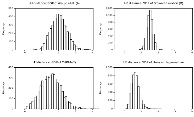
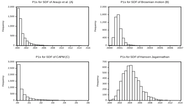
The results from Tables 2 and 3 point to the same findings and, in gen-eral, the model ranking based on artificial returns is B C A. It should be highlighted that the SDF of Hansen-Jagannathan would be the best one across the four presented SDFs, however, it is not considered in the “horse race”, since it is designed to generate an adequate HJ distance, so it is presented here only as a benchmark. For further details regarding these findings, see Figures A.1-A.6 in Appendix containing, for illustrative pur-poses, the histograms for the HJ distance and for the pricing-error-based goodness of fit statistics p1s of each SDF candidate estimator, based on

Fama-French factors and three considered Monte Carlo configurations: (i)

N = 25,T = 280; (ii)N = 48,T = 350; (iii)N = 96,T = 500.

(27)

this variable. Finally, model C is not selected in real data, and usually not suggested in the simulated returns setup, which is a result closely linked to the hypotheses embodied in the CAPM framework (e.g., two-period model and log utility function); revealing that such hypotheses are indeed not re-flected in both real and artificial data.19

6. Conclusions

In this paper, we propose a methodology to compare different stochas-tic discount factor models constructed from relevant market information. Based on a multifactor approach, which is grounded on characteristics of the firms in a particular economy, a Monte Carlo simulation strategy is pro-posed in order to generate a set of artificial returns that is properly compati-ble with those factors. One feature of such methodology is that the compar-ison directly relies on estimated stochastic discount factor time series and their ability to properly price asset returns. One advantage of this approach is to enable investigating the performance of different models based not only on a single realization of asset return series (i.e., real data time series), but also to provide a simulated setup with up ton= 5,000replications of real data in order to compare model performance in a much broader dataset. This approach can mimic observed data features (e.g., time-dependence and covariance structures) and, thus, provide a reality check to evaluate distinct SDFs (White, 2000, see).

Therefore, the main contribution of this paper consists of a methodol-ogy to compare distinct SDFs in a setup where a multifactor approach is used to summarize a given economic environment, which is used to gen-erate numerical simulations in which SDF proxies are compared through a goodness-of-fit statistic and the Hansen and Jagannathan distance. An empirical application is provided to illustrate our methodology, in which returns time series are produced from three set of factors of the U.S. econ-omy.

The main results based on real data quite often indicate the SDF model of Araujoet al.(2006). Its nonparametric setup and data-driven approach lead to a performance improvement as long as the sample sizes increase (i.e., number of considered assets and time periods). Nonetheless, this

re-19_{In addition, provided that simulated data comes from models based on three (or six)}

(28)

sult is not robust when considering simulated datasets within a Monte Carlo exercise. In this case, the SDF of Brandtet al.(2006) seems to be the best model, given that the Brownian motion hypothesis is able to generate SDF dynamics with adequate statistical features, which are closer to the Hansen and Jagannathan SDF. Finally, the CAPM derived SDF is not often indi-cated by the comparison exercise, since its restricted hypotheses, such as the log utility function and single two-period model, seem to be rejected by both real and simulated data.

Future extensions of this paper might also include the investigation of other SDF proxies as well as the adoption of distinct factors. In addition, the analysis of such models in other economies, such as developed or emerg-ing ones, might lead to distinct model recommendations, dependemerg-ing on the adequacy of each model’s assumptions with respect to different market fea-tures. For example, the empirical exercise could be extended to the Brazil-ian stock market. However, market specific features, such as liquidity issues and structural breaks, should properly be taken into account in order to not bias the results regarding the estimated SDFs. For instance, the merge in 2008 of the Brazilian stock market (Bovespa) with the Brazilian Mercan-tile & Futures Exchange (BMF)20resulted in a liquidity break, due to the sudden hike in market liquidity. A formal treatment on this issue (within a factor modeling setup) would require, for instance, the use of dummies and tests for the hypothesis of a time series structural break (e.g., in monthly fi-nancial volume). In order to guide this possible route, some papers focused on factor models and Brazilian data are worth mentioning.21 For instance, Rayeset al.(2012) examine whether the Fama-French (FF) model, applied

20_{BM&FBOVESPA is a Brazilian company, created in 2008, through the integration}

between the S˜ao Paulo Stock Exchange (Bolsa de Valores de S˜ao Paulo) and the Brazilian Mercantile & Futures Exchange (Bolsa de Mercadorias e Futuros). Nowadays, it is the most important Brazilian institution to intermediate equity market transactions and the only securities, commodities and futures exchange in Brazil. It also acts as a key driver for the Brazilian capital markets.

21_{Some related papers are the following: (i) Neves & Leal (2003), which investigate}

the relationship between GDP growth and the effects of size, value and moment within a FF setup; (ii) M´alaga & Securato (2004) corroborate the statistical significance of the three FF factors regarding return forecasts; (iii) Lucena & Pinto (2005) revisit the FF model for Brazilian data and adapt it to include parameters from ARCH-GARCH models; (iv) Mussa

(29)

to investment portfolios with variable weightings, still explains the returns in view of the structural break in the Brazilian stock market in terms of its liquidity.22 Nonetheless, extensions to the presented empirical exercise remain an open route for future research.

References

Ahn, Seung C., & Gadarowski, Christopher. 2004. Small Sample Proper-ties of the GMM Specification Test Based on the Hansen-Jagannathan Distance. Journal of Empirical Finance,11, 109–132.

Ang, Andrew, Hodrick, Robert J., Xing, Yuhang, & Zhang, Xiaoyan. 2006. The Cross- Section of Volatility and Expected Returns. Journal of

Fi-nance,61, 259–299.

Araujo, Fabio, Issler, Jo˜ao V., & Fernandes, Marcelo. 2006. A Stochastic

Discount Factor Approach to Asset Pricing Using Panel Data. Getulio

Vargas Foundation, Ensaios Econˆomicos n. 628, mimeo.

Brandt, Michael W., Cochrane, John H., & Santa-Clara, Pedro. 2006. Inter-national Risk Sharing is Better Than You Think, or Exchange Rates are Too Smooth. Journal of Monetary Economics,53, 671–698.

Campbell, John Y., & Cochrane, John H. 2000. Explaining the Poor Per-formance of Consumption-Based “Asset Pricing Models”. Journal of

Finance,55, 2863–2878.

Campbell, John Y., Lo, Andrew W., & MacKinlay, A. Craig. 1997. The

Econometrics of Financial Markets. Princeton University Press.

Carhart, Mark M. 1997. On Persistence in Mutual Fund Performance.

Jour-nal of Finance,52, 57–82.

Chan, Ka-Keung C., Karolyi, G. Andrew, & Stulz, Ren´e M. 1992. Global

FinancialMarkets and the Risk Premium on U.S. Equity. NBER Working

Paper n. 4074.

Chen, Xiaohong, & Ludvigson, Sydney C. 2009. Land of Addicts? An Empirical Investigation of Habit-Based Asset Pricing Models. Journal

of Applied Econometrics,24, 1057–1093.

22

(30)

Cochrane, John H. 2001. Asset Pricing. Princeton: Princeton University Press.

Daniel, Kent, & Titman, Sheridan. 2012. Testing Factor-Model Explana-tions of Market Anomalies. Critical Finance Review,1, 103–139.

Dittmar, Robert F. 2002. Nonlinear Pricing Kernels, Kurtosis Preference, and Evidence from the Cross Section of Equity Returns. Journal of

Fi-nancial Economics,33, 3–56.

Engle, Robert F., & Kozicki, Sharon. 1993. Testing for Common Features.

Journal of Business and Economic Statistics,11, 369–380.

Fama, Eugene F., & French, Kenneth R. 1992. The Cross Section of Ex-pected Stock Returns. Journal of Finance,47, 427–465.

Fama, Eugene F., & French, Kenneth R. 1993. Common Risk Factors in the Returns on Stocks and Bonds. Journal of Financial Economics,33, 3–56.

Fama, Eugene F., & French, Kenneth R. 1996. Multifactor Explanations of Asset Pricing Anomalies. Journal of Finance,51, 55–84.

Fama, Eugene F., & French, Kenneth R. 1998. Value versus Growth: The International Evidence. Journal of Finance,53, 1975–1979.

Fama, Eugene F., & MacBeth, James D. 1973. Risk, Return and Equilib-rium: Empirical Tests. Journal of Political Economy,81, 607–636.

Farnsworth, Heber, Ferson, Wayne E., Jackson, David, & Todd, Steven. 2002. Performance Evaluation with Stochastic Discount Factors.Journal

of Business,75, 473–503.

Fernandes, Marcelo, & Vieira Filho, Jos´e. 2006. Revisiting the Efficiency of Risk Sharing Between UK and US: Robust Estimation and Calibration

under Market Incompleteness. Mimeo.

Ferson, Wayne E., & Harvey, Campbell R. 1994. Sources of Risk and Expected Returns in Global Equity Markets. Journal of Banking and

Finance,18, 775–803.

(31)

Gaunt, Clive. 2004. Size and Book to Market Effects and the Fama French Three Factor Asset Pricing Model: Evidence from the Australian Stock Market. Accounting and Finance,44, 27–44.

Griffin, John M. 2002. Are the Fama and French Factors Global or Country-Specific? Review of Financial Studies,15, 783–803.

Grinblatt, Mark, & Titman, Sheridan. 2002. Financial Markets and

Corpo-rate StCorpo-rategy. Boston: McGraw-Hill.

Hansen, Lars P., & Jagannathan, Ravi. 1991. Implications of Security Mar-ket Data for Models of Dynamic Economies. Journal of Political Econ-omy,99, 225–262.

Hansen, Lars P., & Jagannathan, Ravi. 1997. Assessing Specification Errors in Stochastic Discount Factor Models. Journal of Finance,52, 557–590.

Hansen, Lars P., & Richard, Scott F. 1987. The Role of Conditioning In-formation in Deducing Testable Restrictions Implied by Dynamic Asset Pricing Models. Econometrica,55, 587–614.

Harrison, John M., & Kreps, David M. 1979. Martingales and Arbitrage in Multiperiod Securities Markets. Journal of Economic Theory,20, 381– 408.

Jagannathan, Ravi, & Wang, Zhenyu. 2002. Empirical Evaluation of Asset-Pricing Models: A Comparison of the SDF and Beta Methods. Journal

of Finance,57, 2337–2367.

Jagannathan, Ravi, Kubota, Keiichi, & Takehara, Hitoshi. 1998. Relation-ship Between Labor-Income Risk and Average Return: Empirical Evi-dence from the Japanese Stock Market. Journal of Business, 71, 319– 348.

Jegadeesh, Narasimhan, & Titman, Sheridan. 1993. Returns to Buying Winners and Selling Losers: Implications for Stock Market Efficiency.

Journal of Finance,48, 65–91.

Johnson, Richard A., & Wichern, Dean W. 1992. Applied Multivariate

(32)

Kan, Raymond, & Robotti, Cesare. 2009. Model Comparison Using the Hansen-Jagannathan Distance. Review of Financial Studies, 22, 3449– 3490.

Lettau, Martin, & Ludvigson, Sydney. 2001a. Consumption, Aggregate Wealth, and Expected Stock Returns. Journal of Finance,56, 815–849.

Lettau, Martin, & Ludvigson, Sydney. 2001b. Resurrecting the (C)CAPM: A Cross-Sectional Test When Risk Premia are Time-Varying. Journal of

Political Economy,109, 1238–1287.

Lucena, Pierre, & Pinto, Antonio. 2005.Estudo de Anomalias No Mercado Brasileiro de Ações Através de Uma Modi.Cação No Modelo de Fama

e French. InEncontro Anual da Associac¸˜ao Nacional de Programas de

P ós-Graduação em Administração, 29, 2005. Bras´ılia: ANPAD.

Málaga, Flavio K., & Securato, José Roberto. 2004. Aplicaç ão Do Modelo de Três Fatores de Fama e French No Mercado Acionário

Brasileiro: Um Estudo Emp´ırico Do Per´ıodo 1995–2003. In

Encon-tro Anual da Associação Nacional de Programas de P ós-Graduação em Administração, 28, 2004. Curitiba: ANPAD.

Marinelli, Federico. 2011. The Relationship Between Diversification and

Firm’s Performance: Is There Really a Causal Relationship?

Univer-sity of Navarra, IESE Business School. Working Paper WP-907, Mimeo. Available at: http://www.iese.edu/research/pdfs/DI-0907-E. pdf.

Mussa, Adriano, Santos, José Odálio Dos, & Famá, Rubens. 2007. A Adição Do Fator de Risco Momento Ao Modelo de Precificaç ão de Ativos Dos Três Fatores de Fama & French, Aplicado Ao Mercado Acionário

Brasileiro. InCongresso USP de Controladoria e Contabilidade, 7, S˜ao

Paulo. S˜ao Paulo: USP.

Mussa, Adriano, Rogers, Pablo, & Securato, José Roberto. 2009. Modelos de Retornos Esperados No Mercado Brasileiro: Testes Emp´ıricos Uti-lizando Metodologia Preditiva. Revista de Ciências da Administraç ão,

11, 192–216.

(33)

Mo-mento? InEncontro Anual da Associação Nacional de Programas de P ós-Graduação em Administração, 27, 2003. Atibaia: ANPAD.

Newey, Whitney K., & West, Kenneth D. 1987. A Simple, Positive Semi-Definite, Heteroskedasticity and Autocorrelation Consistent Covariance Matrix. Econometrica,55, 703–708.

Newey, Whitney K., & West, Kenneth D. 1994. Automatic Lag Selection in Covariance Matrix Estimation. The Review of Economic Studies, 61, 631–653.

Perez-Quiros, Gabriel, & Timmermann, Allan. 2000. Firm Size and Cycli-cal Variations in Stock Returns. Journal of Finance,55, 1229–1262.

Rayes, Ana Cristina W., Ara´ujo, Gustavo S., & Barbedo, Claudio S. 2012. O Modelo de 3 Fatores de Fama e French Ainda Explica Os Retornos No Mercado Acion´ario Brasileiro? Revista Alcance,19, 52–61.

Ren, Yu, & Shimotsu, Katsumi. 2006. Specification Test Based on the

Hansen-Jagannathan Distance with Good Small Sample Properties.

Queen’s University. Mimeo.

Ross, Stephen A. 1976. The Arbitrage Theory of Capital Asset Pricing.

Journal of Economic Theory,13, 341–360.

Sharpe, William F. 1964. Capital Asset Prices: A Theory of Market Equi-librium under Conditions of Risk. Journal of Finance,19, 425–442.

Stock, James H., & Watson, Mark W. 2002. Forecasting Using Principal Components from a Large Number of Predictions. Journal of the

Amer-ican Statistical Association,97, 1167–1179.

Tucker, Ledyard, & MacCallum, Robert. 1993. Exploratory Factor

Anal-ysis – A Book Manuscript. Available at_{http://www.unc.edu/~rcm/}

book/factornew.htm.

White, Halbert. 2000. A Reality Check For Data Snooping. Econometrica,

(34)

[image:34.595.76.368.404.495.2]

Appendix

Table A.1

Descriptive statistics of the SDF proxies

Three factor Rm, SMB and HML of Fama and French N=25 and T=280

Araujo Brownian Motion CAPM HJ

Mean 0,9942 0,9269 0,9855 0,9872

Median 0,9888 0,7504 1,0254 0,9866

Maximum 1,2614 9,4122 1,9549 3,1385

Minimum 0,8783 0,1295 -0,9218 -0,9362 Std. Dev 0,0473 0,7437 0,3735 0,5503 Skewness 1,1698 4,9300 -0,8163 0,0618 Kurtosis 7,7475 50,1766 5,5646 3,6060 Freq. Jarque-Bera 0,0000 0,0000 0,0000 0,5000

Six factor Rm, SMB, HML, Mom, STRev and LTRev of Fama and French N=48 and T=280

Mean 0,9919 0,9234 0,9847 0,9867

Median 0,9867 0,7516 0,8718 0,9947

Maximum 1,2534 8,1673 7,5042 2,7757

Minimum 0,8750 0,1341 -2,8876 -0,7856 Std. Dev 0,0470 0,7124 1,3491 0,5371 Skewness 0,9917 4,0046 0,0000 -0,0558 Kurtosis 7,4733 39,6145 5,5646 3,3564 Freq. Jarque-Bera 0,5000 0,0000 0,0000 0,5000

T = 280 and three factor obtained of the S&P500 using the factor model. Eigenvalue: lambda1 = 0.6473, lambda2 = 0.1482 and lambda3 = 0.0961. N=96 and T=280

Mean 0,9945 0,9206 0,9856 0,9877

Median 0,9862 0,7757 1,0084 0,9824

Maximum 1,2764 4,3482 1,3458 2,1626

Minimum 0,8633 0,2451 0,1677 -0,3410 Std. Dev 0,0564 0,5392 0,1619 0,3870 Skewness 1,0957 2,0823 -1,0912 -0,0066 Kurtosis 7,3363 10,5206 5,9640 3,2155 Freq. Jarque-Bera 0,5000 0,0000 0,0000 1,0000

Notes: These statistics are computed in-sample. The descriptive statistics are

(35)

0 100 200 300 400 500

.0 .1 .2 .3 .4

F re q u e n c y

HJ distance: SDF of Araujo et al. (A)

0 200 400 600 800 1,000 1,200

.0 .1 .2 .3 .4

F re q u e n c y

HJ distance: SDF of Brownian motion (B)

0 100 200 300 400

.0 .1 .2 .3 .4

F re q u e n c y

HJ distance: SDF of CAPM (C)

0 200 400 600 800 1,000

.0 .1 .2 .3 .4

F re q u e n c y

[image:35.595.65.373.56.242.2]

HJ distance: SDF of Hansen Jagannathan

Figure A.1

Histogram of the HJ distance forN= 25andT= 280

0 100 200 300 400 500 600

.0 .1 .2 .3 .4

F re q u e n c y

0 250 500 750 1,000 1,250 1,500

.0 .1 .2 .3 .4

F re q u e n c y

0 100 200 300 400 500 600

.0 .1 .2 .3 .4

F re q u e n c y

0 200 400 600 800 1,000

.0 .1 .2 .3 .4

F re q u e n c y

[image:35.595.65.374.310.496.2]

Figure A.2

(36)

0 100 200 300 400 500 600

.0 .1 .2 .3 .4

F re q u e n c y

0 400 800 1,200 1,600 2,000

.0 .1 .2 .3 .4

F re q u e n c y

0 100 200 300 400

.0 .1 .2 .3 .4

F re q u e n c y

0 200 400 600 800 1,000 1,200

.0 .1 .2 .3 .4

F re q u e n c y

[image:36.595.66.372.56.242.2]

Figure A.3

Histogram of the HJ distance forN= 96andT= 500

0 400 800 1,200 1,600 2,000 2,400 2,800

.000 .004 .008 .012 .016 .020 .024 .028

F re q u e n c y

P1s for SDF of Araujo et al. (A)

0 200 400 600 800 1,000 1,200

.0000 .0002 .0004 .0006 .0008 .0010

F re q u e n c y

P1s for SDF of Brownian m otion (B)

0 1,000 2,000 3,000 4,000

.00 .01 .02 .03 .04 .05 .06 .07 .08 .09 .10 .11

F re q u e n c y

P1s for SDF of CAPM (C)

0 100 200 300 400 500 600

.000 .005 .010 .015 .020 .025 .030 .035

F re q u e n c y

P1s for SDF of Hansen Jagannathan

Figure A.4

[image:36.595.65.372.312.491.2]

(37)

0 250 500 750 1,000 1,250 1,500

.000 .002 .004 .006 .008 .010 .012 .014 .016 .018

F re q u e n c y

0 200 400 600 800 1,000 1,200

.0000 .0001 .0002 .0003 .0004 .0005 .0006

F re q u e n c y

0 100 200 300 400 500 600

.000 .004 .008 .012 .016 .020 .024 .028 .032

F re q u e n c y

0 100 200 300 400 500 600

.000 .002 .004 .006 .008 .010 .012 .014 .016 .018

F re q u e n c y

[image:37.595.66.370.55.233.2]

Figure A.5

Histogram of thegoodness-of-fit statisticp1sforN= 48andT = 350

0 500 1,000 1,500 2,000

.000 .002 .004 .006 .008 .010 .012 .014 .016

F re q u e n c y

0 400 800 1,200 1,600 2,000

.0000 .0001 .0002 .0003 .0004 .0005 .0006 .0007

F re q u e n c y

0 500 1,000 1,500 2,000 2,500 3,000

.00 .01 .02 .03 .04 .05 .06

F re q u e n c y

0 100 200 300 400 500 600 700

.000 .002 .004 .006 .008 .010 .012 .014

F re q u e n c y

Figure A.6

[image:37.595.65.372.312.492.2]