Munich Personal RePEc Archive
Assessing bank’s default probability
using the ASRF model
Radkov, Petar and Minkova, Leda
Faculty of Mathematics and Informatics, Sofia University "St. Kl.
Ohridski"
25 June 2011
Online at
https://mpra.ub.uni-muenchen.de/60186/
Assessing bank’s default probability using the
ASRF model
Petar Radkov
Leda Minkova
Faculty of Mathematics and Informatics
Sofia University ”St. Kl.Ohridski”
Abstract
In this paper it is shown how a Vasicek-model approach and the assumptions in
Basel 2 regulatory framework can be used to develop measures of the probability of
banks’ failure. The Basel 2 framework is based on a Vasicek-model approach. The
estimation of the propose measure of bank probability of default could be made over
the capital ratio from supervisory authorities (non-public information) or over the
capital ratio from balance sheet data (public available information).
Key words: Vasicek model, ASRF model, Basel 2, banks’ probability of default
Mathematics Subject Classification 2000: 60J05; 60J10; 60J20; 91B24.
1
Introduction
The Vasicek-model approaches and the assumptions in Basel 2 regulatory framework could
be used to develop measures of the probability of banks’ failure. Capital requirements’
set by Basel 2 are based on standardize approach or advanced internal risk based (IRB)
approach. The banks’ probability of default measure could be extracted by the capital ratio
from balance sheet data (public available information).When we know the probability of
default of loans portfolio according to the Vasicek-model approach (see Vasicek 2002) we
could calculate the requirement bank capital equal to 99.9The modified model could be used
to estimate the banks’ probability of default where the IRB approach set by Basel 2 is not
accepted from regulatory institutions or the banks do not use it.
The remainder of this paper is organized as follows. The second section presents a brief
review .. In the third section we describe our model.
2
Background
Usually in practice there are two alternative methodologies for estimating the probability
of default. The first one is based on the historical data analysis. The second is based on
the conception of imply probability measure from the option pricing theory, developed by
Merton (1974) and then continuing by Vasicek (1987). The last method is extended by
Basel 2 as a regulatory framework to valuate the loss on loan portfolio and to calculate
requirement capitals. This paper is closely related to the second concept for quantifying the
banks probability of default.
3
Methodology
Basel 2 takes the Vasicek model which is used to determine the regulatory capital in the
Basel 2 framework. Under the assumptions of the model could be estimate the expected loss
(EL) and unexpected loss (UL) of the banks. The expected loss is determined by three main
ingredients: Probability of default (PD), Exposure at default (EAD) and Loss given default
(LGD). The EAD means the amount of money owed at the moment counterparty goes into
default. The LGD is the percentage of the EAD lost during a default. The expected loss is
EL=P D∗EAD∗LGD
(1)
and determines the amount of provisions which should be taken by the banks as a reserves.
The UL is the additional loss in nonregular circumstances, for which tier capital should be
retained. In the Vasicek model approach the UL is defined by the PD in a downturn situation.
The model assumes that the EAD and LGD are not affected by dire circumstances. The
both parameters are considered constant for a company.
VaR is defined as a threshold value x such that the probability of exceedance x is equal
to α < 1. α is called a confidential level. Basel 2 uses VaR coefficient as a measure of risk.
The VaR is obtained by algebraically inverting the distribution function F(x)
P(L≤x) = F(x),
(2)
where x is set to be equal to the maximum losses (Value at Risk). Basel 2 sets the probability
1−α equal to 0.999 (BIS 2005) and V aR99.9 is equal to x=F−1(0.999).
The unexpected loss is calculated as following
U L=V aR99.9−P D∗LGD
(3)
More specifically, the new capital accord uses the Vasicek result to compute the Value at
Risk (VaR) for each obligor, which is the maximum loss amount that is not expected to be
exceeded with a given level and within a defined time horizon. In general the banks are
expected to cover their expected loss on an ongoing basis by provisions and write-offs
while Basel 2 requires banks to hold capital only to protect against unexpected losses.
Our task is to assess banks’ default probability from the banks’ required capital or capital
from the balance sheets. That is an inverting problem of Vasicek model. VaR is computed
of each obligor is known. The estimation of the proposed measure of bank probability of
default could be made over the capital ratio from supervisory authorities (non-public
infor-mation) or over the capital ratio from balance sheet data (public available inforinfor-mation). The
assumptions under which we calculate the implied probability of default are the following:
• Banks portfolios are exposed only to the credit risk, Banks’ credit portfolio is
homo-geneous and the portfolio is infinitely divisible,
• The maximum loss (VaR) is set by Basel 2 to be equal to 99.9
• Required capital determinate by standardized approach or by internal rating based
approach IRB (foundation and advanced approaches) both of them base on Basel 2 is
a sufficient to cover the unexpected loss in 0.999.
The basis of the Basel 2 IRB approach is the Vasicek portfolio credit loss model (Vasicek,
1987, Vasicek, 2002). Vasicek offers one factor model which was firstly introduce by Merton
in 1974 . Consider a portfolio consisting of n loans. Dynamic of the value of the assets of a
borrower ifor i= 1,2, ...n can be described by the geometrical Brownian motion:
dAi =µAi(t)dt+σAi(t)dWi(t)
(4)
where W(t) is a Wiener process and W(t) N(0, t).
Thus the value of assets at time T can be expressed as:
Ai(T) = Ai(0)e(µ− σ2
2 )T+σ
√
T W(T)
(5)
Basel’s 2 formula uses Merton’s model interpretation of default probability of the
bor-rower i, so an obligor will default if the value of his assets falls below the value of his debt:
p=P(Ai(T)< Bi) = P(Wi < ci) = N(ci) = N(−di)
(6)
ci =
ln(Bi/Ai)−(µ+σ
2
2 )T
σ√T
(7)
where N(−d2) is the standard normal distribution function giving the default probability
which is equal to p. Then p=N(ci) and thereforeci =N−1(p). For fixed t we assume that
Wi has the following expression:
Wi =by+aεi
(8)
where y represents systemic risk affecting the entire portfolio and is the specific risk for
borrower i. It is assumed that both of them follow standard normal distributions. The
values of b and a are given by:
b=√ρ a=p1−ρ
(9)
where ρ measures the asset correlation between borrowers’ assets. It could be described
as the dependence of the assets of a borrower on the general state of the economy; so
all borrowers are linked to each other by the single risk factor, etc the common pairwise
correlation between obligors (see Vasicek 1991).
Under those conditions, default probability of any loan, conditional on the single risk
factor y, can be written as:
P(x|y) = P(by+aεi < ci) = P
εi <
ci−by
a
P(x|y) =P
εi <
ci −by
a
=P
εi <
N−1(p)−√ρy
√
1−ρ
We can establish that the percentage of default on total portfolio equals the number of
individuals that default divided by total number of obligators. If n is large enough, by the
law of the large numbers it can be stated that the fraction of clients x that default is equal
to the default probability conditional on y (4).
Under certain homogeneity assumptions, the Vasicek model leads us to very simple
an-alytic asymptotic approximation of loss distribution due to each obligor (see Vasicek 2002).
The cumulative distribution function of loan losses L on a very large portfolio is given by
the limit:
P(L≤x) = F(x) =N
√
1−ρN−1(x)−N−1(P D)
√ρ
(11)
where N is the standard normal distribution function. We use the notation PD for the
probability of default, previously noted by p.
According to the Basel 2, if the LGD is equal to 1, 0.999 VaR (BIS 2005) has the following
representation:
V aR99.9 =N
r
1 1−ρN
−1(P D) +
r ρ
1−ρN
−1(0.999)
(12)
the loss could be recovered, i.e. the LGD is not equal to 1 then
V aR99.9 =LGD∗N
r
1 1−ρN
−1(P D) +
r
ρ
1−ρN
−1(0.999)
(13)
The VaR quantity represents the basis for the computation of the bank capital
require-ment.
Then from (3) and (6) we get the formula for calculating capital requirements, known as
a capital allocation parameter:
C=
LGD∗N
r
1 1−ρN
−1(P D) +
r ρ
1−ρN
−1(0.999)
−P D∗LGD
According to the Basel 2 the formula (7) is adjusted to the following result
C =hLGD∗Nhq11
−ρN
−1(P D) +q ρ
1−ρN
−1(0.999)
i
−P D∗LGDi
(1−1.5B)−1[1 + (M−2.5)B]1.06,
where M is the time to maturity and B is a function of PD computed as
B = [0.11852−0.05478 ln(P D)]2
The equation (8) represents the adjusted capital in order to take into account the expected
loss and the maturity adjustment factors.
According to the Basel 2 the correlation coefficient ρ is given by:
ρ = 0.121−e−50P D
1−e−50 + 0.24 h
1− 1−e−50P D
1−e−50 i
−0.04
1− S−5
45
,
where S is the size of the firm.
Given the assumption of the infinite divisibility, the overall capital requirement for a
bank is computed as a sum of the capital requirements of each loan exposure:
K =X
i
Ci(P Di)Ai
(15)
that is the sum of the capital allocation parameter Ci of each exposure i multiplied by its
amount Ai. If the credit portfolio is homogenous then there is one implied probability of
default which could be extracted from capital adequacy ratio:
K
P
iAi
=C(P D∗) (16)
We can derive the averageP D∗ of a banks’ credit portfolio as a function of capital
P D∗ =fXA
i, K
(17)
estimate the implied probability of default by equation (13) under the previous assumptions.
The capital ratio could be taken from supervisory authorities as a non-public information
(capital adequate ratio) or from balance sheet data as a public available information.
4
Numerical examples
Coming after the described method for assessing the implied probability, we implement it in
MatLab. We find out the implied probability of default as a function of capital ratio, given
in Figure 1. The function of implied probability of default vs. capital ratio is an increasing
function which describes the fact that more risk taken from the bank costs more capital to
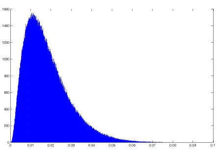
it.The loss distribution as a function of default probability is given in Figure 2. The loss
distribution has been found with 1 million Monte Carlo simulations.
5
Conclusion
This paper describes the derivation of implied default probabilities from the Vasicek model
and Basel 2 framework. Our method for measuring probability of default is very simple and
easy to implement in the both cases when we use the capital ratio from balance sheet data
(public available information) and the capital ratio from supervisory authorities (non-public
information).
Once we know the implied probability of default we could get the following: 1. Find
out the loss distribution via Monte Carlo simulations (Figure2); 2. Find out the expected
loss which should be coved by provisions and write-offs. 3. Make simulations and stress
tests what will happen if the probability of default rose sharply for one bank or for the total
Figure 1: The relation between implied probability of default as a function of capital ratio
[image:10.612.195.416.309.468.2]Acknowledgments
The authors were partially supported by the Bulgarian NSRF grant DTK 02/71, 2011.
References
[1] BIS (1999), Credit Risk Modeling: current practices and applications - April
[2] BIS (2003), Overview of the new Basel capital accord, Consultative document- April
[3] BIS (2004), Modifications to the capital treatment for expected and unexpected credit
losses- January
[4] BIS, (2004), International Convergence of Capital Measurements and Capital Standards:
A Revised Framework, Basel Committee on Banking Supervision (referred to as Basel
II), June.
[5] BIS (2005), An explanatory note on the Basel II IRB Risk Weight Functions - July
[6] Merton, R., (1974), On the Pricing of Corporate Debt: The Risk Structure of Interest
Rates, Journal of Finance, 29, pp. 449-470
[7] Vasicek O, (2002), Loan portfolio value, Risk December, 160-162.
[8] Vasicek O, (1991), Limiting Loan Loss Probability Distribution, KMV Corporation