The Poset Cover Problem
Lenwood S. Heath1, Ajit Kumar Nema2 1Department of Computer Science, Virginia Tech, Blacksburg, USA 2Core Quantative Strategies, Goldman Sachs, India Pvt. Ltd., Bangalore, India
Email: [email protected], [email protected]
Received March 1, 2013; revised April 1, 2013; accepted May 15, 2013
Copyright © 2013 Lenwood S. Heath, Ajit Kumar Nema. This is an open access article distributed under the Creative Commons Attribution License, which permits unrestricted use, distribution, and reproduction in any medium, provided the original work is properly cited.
ABSTRACT
A partial order or poset P
X,
on a (finite) base set X determines the set
P of linear extensions of P. The problem of computing, for a poset P, the cardinality of
P is #P-complete. A set
P P1, , ,2 Pk
of posets onX covers the set of linear orders that is the union of the
Pi . Given linear orders L L1, , ,2 Lm on X, the PosetCover problem is to determine the smallest number of posets that cover
L L1, , ,2 Lm
. Here, we show that thedecision version of this problem is NP-complete. On the positive side, we explore the use of cover relations for finding posets that cover a set of linear orders and present a polynomial-time algorithm to find a partial poset cover.
Keywords: Linear Orders; Partial Orders; NP-Completeness; Algorithms
1. Introduction
Finite partial orders or posets have numerous applica- tions, including scheduling [1-8], molecular evolution [9-12], data mining [13-17], graph theory [18-23], and algebra [24-27]. Many applications implicitly or explic- itly involve linear extensions of posets. For example, the solution of many scheduling problems requires a lineari- zation of the jobs being scheduled consistent with some precedence constraints given by a poset. As the number of linear extensions of a poset may be exponential in the number of elements of the base set, many computational problems related to linear extensions are not solvable in polynomial time. Ruskey [28], West [29], Pruesse and Ruskey [30], Canfield and Williamson [31], Korsh and LaFollette [32], and Ono and Nakano [33] provide algo- rithms to generate all of the linear extensions of a finite poset. As the size of a solution may be exponentially large, these algorithms emphasize the ability to generate each successive linear extension in polynomial time, at least on average. Sampling the linear extensions of a poset is easier. Bubley and Dyer [34] use a rapidly mix- ing Markov chain to generate a random linear extension of a finite poset, sampled almost uniformly.
Problems in mining order information from databases of sequences (see, e.g., [16,17,35,36]) have an inverted character from that of many computational problems
involving posets. Here, a problem instance is a set of linear orders of items from some universal set, while a solution is one or more posets that well explain, through their linear extensions, a significant number of the linear orders. An example from computational neuroscience [37] might go as follows. Each item is the firing of a neuron, while each linear order is a sequence of neuronal firings, ordered in time from an experiment. The solution is a neural circuit that explains a set of such linear orders. These novel problems are ripe for mathematical formal- ization and study. In this paper, we define and study one such problem. A problem instance is a set of permuta- tions of a base set, and a solution covers the instance with linear extensions (Section 2). We prove that the Poset Cover problem (a decision problem) is NP-com- plete in Section 3. In Section 4, we explore how cover relations relate to poset covers. Finally, we develop a polynomial-time algorithm to find a partial cover in Sec- tion 5.
2. Preliminaries
In this section, we establish terminology and notation and prove some basic results.
A partial order or poset P is an irreflexive, anti-
ordered pair P
X,P
. Equivalently, poset P is atransitive directed acyclic graph (DAG), namely,
, , P
P X x y x y . If G is a DAG, then its transi- tive closure is a poset by this equivalence. The rank
function P:X
1, 2, , n
is given by
1
P x y y Px
. The empty poset is
X,
.Let x y X, be distinct. Then x and y are com-
parable in P, written xP y, if xP y or yP x,
while x and y are incomparable, written x yP , other- wise. Moreover, x is covered by y or ycovers x, written
P
x y, if xP y and there is no z X such that P P
x z y. In this case, the ordered pair
x y, is acover relation for P. It is well-known that a (finite)
poset is uniquely determined by its set of cover relations (see [38]).
If P1
X,P1
and P2
X,P2
are posets on thesame set X, then P2 is an extension of P1, written
1 2
PP , if, for all a b X a, , P1b implies aP2 b.
The relation on posets of X is reflexive, antisym- metric, and transitive.
A linear order L
X,L
on X is a poset L suchthat, for x y X, , either x y or xL y holds. If L is a linear order, then the rank function
: 1, 2, ,
L X n
is a bijection. Setting 1
i L x i ,
L can be written as the sequence L x x 1, , ,2 xn,
which is a permutation of X. Also, we write L i
for the element of rank i in L. A linear extension L of a poset P is a linear order such that PL. The set of all linear extensions of P is
P . Note that
is the set of all linear orders on X . Brightwell and Winkler [39] prove that the problem of determining
P for a poset P is #P-complete.
Let
P P1, , ,2 Pk
be a set of k posets on X.This set covers the set of linear orders
1 .
k i i
P
A poset P is maximal in if
P and there is no poset P of X such that PP P, P, and
P . Let be a set of posets on X, and let be a set of linear orders on X. blankets if
.P
P
Lemma 1 Let be the set of linear orders that is
covered by a set of posets of cardinality k. Then,
there exists a cover ˆ of cardinality k k that also
covers such that every poset in ˆ is maximal in
.
Proof. We construct ˆ by examining each poset in
. Let P. If P is maximal in , then add P
to ˆ. Otherwise, let P be a poset of minimum car- dinality (as a set of ordered pairs) such that PP and
P . Since P is not maximal, P P . More-
over, any poset P contained in P of smaller car- dinality will have
P . Add P to ˆ.The constructed ˆ has cardinality k. Moreover, ˆ
also covers and every poset in ˆ is maximal in . The lemma follows.
In this paper, we are interested in reversing the cover relationship by addressing the problem of finding a minimum set of posets that covers a given set of linear orders. As a decision problem, this is
Poset Cover
INSTANCE: A base set X of cardinality n1; a nonempty set
L L1, , ,2 Lm
of linear orders overX ; and an integer K m .
QUESTION: Is there a set of posets on X of
cardinality K that covers ?
This problem is shown to be NP-complete in Section 3.
Let L x x 1, , ,2 xn be a linear order on X . For
each i satisfying 1 i n 1, the i-swap of L is the linear order Swap ;
L i x x1, , ,2 xi1,xi1, ,x xi i2, , xn.Let L Swap ;
L i . Evidently, LSwap
L i; , so thei-swap relation is symmetric, written LiL. For
pairs
L L,
that are i-swaps of each other, for somei, we define the function SwapIndex
L L,
i. Note that the set differences of L and L, namely
1
\ i, i
L L x x and L L\
xi1,xi
, each consistof a single ordered pair. In this case, the swap pair for
L and L is the unordered pair
1
SwapPair L L, x xi, i ; otherwise,
SwapPair L L, . Two linear orders L1 and L2
differ by a swap, written L1L2, if 1 2
i
L L , for some i. Since L1L2 if and only if L1L2, the
relation is also symmetric. If L1L2, aL1b,
and bL2a , then we write L2SwapL a b1; ,
tomean that L1iL2 for some i, where the elements swapped are a and b.
Let be a set of linear orders on X. The swap
graph of is the undirected graph
,
L L L,
L
. An edge
L L,
of
is labeled SwapPair
L L,
. Let P be a poseton X, and let L . Then, P is a partial cover of
including L if L
P and
P . The swap graph is the same as the adjacent transpositiongraph of Pruesse and Ruskey [30]. The swap graph of
is bipartite, since every edge connects an even per- mutation to an odd permutation. Moreover, the swap graph
P
of the linear extensions of a single poset is connected (see [30]).Let be the set of all posets on X . Let
A X X be a set of ordered pairs. The up-set of A
Up A P a Pbfor all a b, A .
Up A is empty if and only if the directed graph
X A,
contains cycles. Let
, , and
B a b a b X a b be a set of unordered pairs. The down-set of B is
Down B Pa bP for all a b, B .
Down , and we always have the empty poset
Down B
.
If Up
A = , then define the minimal element in
Up A to be
Up
Min .
P A
A P
The following properties of Min
A follow directly from the definitions.Lemma 2 AMin
A and
Up A PMin A P .
We have the following properties of up-sets and down- sets.
Lemma 3 Let A B, X X. If AB, then
Up B Up A . Let
, , , and
C D c d c dX c d . If CD, then
Down D Down C .
Proof. Suppose that AB. By the definition of up-
sets,
Up < for all ,
< for all , Up .
P
P
B P a b a b B
P a b a b A A
Now, suppose that CD. Then,
Down for all ,
for all , Down ,
P
P
D P a b a b D
P a b a b C C
by the definition of down-sets.
3.
NP
-Completeness of Poset Cover
In this section, we show that PosetCover is NP-complete, in the process using the following known NP-complete decision problem [40].
Cubic Vertex Cover
INSTANCE: A nonempty undirected graph
,
G V E that is cubic, that is, in which every vertex has degree 3; and an integer KV .
QUESTION: Is there a subset V V of cardinality
K
such that every edge in E is incident on at least one vertex in V?
Theorem 4 Poset Cover is NP-complete.
Proof. We show that Poset Cover is in NP and that
Cubic Vertex Cover reduces to Poset Cover in poly- nomial time.
We first show that Poset Cover is in NP. Let X,
L L1, , ,2 Lm
, and K constitute an instance of
Poset Cover, and let
P P1, , ,2 Pk
be a set ofposets on X. First, it is easy to check whether k K in time polynomial in n and m; if kK, then return No. Second, if the cardinality check succeeds, check whether covers as follows. For each poset Pi
in turn, use the Korsh and LaFollette [32] algorithm to generate all the linear extensions of Pi, one at a time, in
constant time per linear extension. As each linear ex- tension L
Pi is generated, check whether L .If not, then return No. If so, then mark that element of
Covered. Note that the number of linear orders
generated by a run of the Korsh and LaFollette algorithm before completion or returning No is at most m. Hence, the worst-case time for one run of the algorithm, in- cluding the checking, is O mn
. Once all the posets and their linear extensions are processed, check whether every element of is marked Covered. If so, then re- turn Yes; otherwise, return No. We find that the worst- case time to check whether covers is
2
O m m n , since k K m . This is polynomial in the size of the original instance. We conclude that Poset Cover is in NP.
Now, let G
V E,
and K constitute an instance of Cubic Vertex Cover . Without loss of generality, assume that V and that V
1, 2, ,
. Let3 2
s E , and let E
e e1, , ,2 es
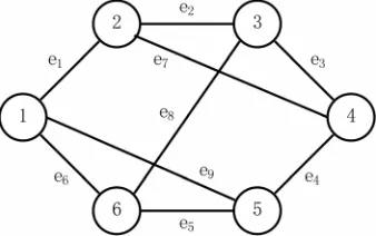
be an arbitrarylabeling of the s edges of G. As a running example of our reduction, we provide the cubic graph in Figure 1, with 6 vertices and s9 edges. To complete the instance of Cubic Vertex Cover , set K4.
Let n2
s2
, and let X
x x1, , ,2 xn
be abase set of n elements. Let Lb, the base order, be the
linear order on X specified by
1 Lb 2 Lb Lb n.
x x x
We view the elements of X as consisting of s2 adjacent, non-overlapping pairs. Specifically, the pairs are x2 1i and x2i, where 1 i s 2. All elements of
[image:3.595.339.508.603.709.2] are obtained by a small set of swaps of such pairs, applied to Lb.
The first s pairs correspond to the s edges in a natural way. In particular, edge eiE is associated with the
edge order Lei Swap
Lb; 2 1i
. Continuing the ex-ample, we set n2
s2
22,
1, , ,2 22
, b 1, , ,2 22,X x x x L x x x
and, for example,
1 2 1 3 4 5 6 7 8 9 10 11 12
13 14 15 16 17 18 19 20 21 22
, , , , , , , , , , , ,
, , , , , , , , , .
e
L x x x x x x x x x x x x
x x x x x x x x x x
For each vertex v V , there are three edges incident on v; let the indices of those edges be
v,1 , v, 2 , and
v,3 . For each pair e v i, and e v j, of these edges, we define the pair edge order to be v i, , v j, Swap Swap ; 2
, 1 ; 2
, 1 .e e b
L L v i v j
For the running example, there are 18 pair edge orders. For each triple e v,1,e v,2 , and e v,3 , we define the
triple edge order to be
,1, ,2, ,3
Swap Swap Swap ; 2 , 1 ; 2 , 1 ;
2 , 1
v v v
e e e
b
L
L v i v j
v k
For the running example, there are 6 triple edge orders.
The primary orders are the base, edge, pair edge, and
triple edge orders. For primary pair edge order Le ei,j ,
there is a corresponding secondary pair edge order ob- tained by swapping x2 1s and x2s2, which is
, Swap i, j; 2 1 .
e ei j e e
L L s
For primary triple edge order Le e ei, ,j k, there is a corre-
sponding secondary triple edge order obtained by
swapping x2s3 and x2s4, which is
, , Swap , , ; 2 3 .
i j k i j k
e e e e e e
L L s
For the running example, there are 18 secondary pair edge orders and 6 secondary triple edge orders.
Collect the various orders into five sets, as follows:
,1,1 ,2,2 ,3,3
,
,
, ,
, ,
1 ,
and are incident on some ,
and are incident on some ,
,
.
i i j
i j
v v v
v v v
e
e e i j
e e i j
e e e
e e e
A L i s
B L e e v V
B L e e v V
C L v V
C L v V
We can now complete our instance of Poset Cover by setting
Lb A B B C C
and setting the integer parameter K K 4. Note that
1 s 8
. For the running example,
4 4 6 28
K and 1 9 8 6 58.
It remains to show that an instance of Cubic Vertex Cover is a Yes instance if and only if the corresponding instance of Poset Cover is a Yes instance.
Fix an instance G
V E,
and K of Cubic Vertex Cover . Let X,, and K constitute the corresponding instance of Poset Cover, as constructed above. By Lemma 1, we may assume that every element of a cover of is maximal in . Since the elements of B must be blanketed by any cover, we may assume that the set
Le ei, j Le ei,j eiandej incident on somev V
is a subset of . Similarly, since the elements of C must be blanketed by any cover, we may assume that the set
Lev,1,ev,2,ev,3 Lev,1,ev,2,ev,3 v V
is a subset of . Note that 4 and that
blankets B B C C.
First, assume that V V is a vertex cover of G of cardinality at most K. Define
b e v,1,e v,2,e v,3
.v V
L L
Note that 4V4 K K and that, by previous observations, it suffices to demonstrate that
blankets Lb and A. Since G is nonempty, E 0, and V 0. Therefore, Lb is blanketed by each of the
posets
,1, ,2, ,3
v v v
b e e e
L L in corresponding to a
vertex v V . For an edge eiE, there is a v V
incident on ei. Then, Lei is blanketed by the poset v,1, v,2, v,3
b e e e
L L in , and hence every linear order
in A is blanketed by . We conclude that covers , as desired.
Now, assume that is a cover of of cardinality at most K. By previous observations, we must have
, for some set of cardinality at most K. Since covers , must blanket Lb and A.
Let ei be any edge of G, incident on vertices u and
v. Without loss of generality, we may assume that
,1
,1i u v . There are two maximal posets that
blanket
,1, ,2, ,3
:
i u u u
e b e e e
L L L and
v,1, v,2, v,3
b e e e
L L . One of these posets must be in .
Moreover, we may assume that contains only orders of this form, since each such order blankets Lb, and the
Define
b e w,1,e w,2,e w,3
.V w V L L
Because blankets all of the Lei’s, we conclude
that V is a vertex cover of G of cardinality V K, as desired.
The theorem follows.
4. Cover Relations
In this section, we examine properties of cover relations in linear orders and their consequences for poset covers.
Let P
X,P
be a poset, thought of as a transitiveDAG. Then, a topological sort of P yields an order
1, , ,2 n
x x x on X such that xiPxj implies i j.
Assume that P is not a linear order. Then there exist ,
a b X such that a bP . There exists at least one
topological sort of P in which a appears to the left of b, and there exists at least one topological sort of P in which b appears to the left of a. (This follows from alternate choices available to the depth-first search used to construct a topological sort. See [41].) Select a topological sort that makes a x i and b x j, where
i j. In that case, we obtain a proper extension P of
P in which a x i P xjb by adding
x xi, j
tothe DAG and taking the transitive closure. Moreover, we have aPb, since the existence of c such that
P P
a c b contradicts a bP . We have just demon-
strated the following.
Lemma 5 Let P
X,P
be a poset, and let,
a b X satisfy a bP . Let
,
, and
.P P a b x y x Pa b P y
Then P
X,P
is a poset, PP, and aPb.Theorem 6 Let P
X,P
be a poset that is not alinear order, and let a b X, satisfy aPb. Then
there exists a proper extension P
X,P
of Psuch that aPb.
Proof. First, suppose that there exists a c X that is
incomparable to a. By Lemma 5, there exists a poset P such that PP and cPa. Moreover,
P P
c a b, so, by the definition of P,aPb.
Second, the case of there being a c X that is incomparable to b is handled analogously.
Finally, we have the case that no element is incom- parable either to a or to b. Let ,c dX be such that
a b, c d, and c dP . (Such a pair ,c d must exist, since P is not a linear order.) If either cPa and dPa or bPc and bPd , then adding
c d, to the DAG for P and taking the transitive closure gives us the desired poset. The case cPa andP
b d (or vice versa) is impossible, since c dP and
P
a b. There are no other cases, since aPb.
The theorem follows.
Theorem 7 Let P
X,P
be a poset, and let,
a b X satisfy a bP . Then there exists a linear order
, L
L X such that L
P and aLb. More-over, for every linear extension L1
X,L1
of P inwhich aL1b, there exists a unique linear extension
2
2 , L
L X of P such that L1L2 and bL2a.
Proof. By Lemma 5, there exists a poset P such that
PP and aPb. By applying Theorem 6 iteratively
to P, we ultimately obtain a linear order L that is an extension of P (and hence of P) such that aLb.
Now, let L1
X,L1
be a linear extension of P inwhich aL1b. Let iL1
a ; then L1
b i 1. Let
2
2 Swap 1; , L
L L i X . Let
1\ , , P
P L a b X . Then P is a poset on X
such that PP and such that a and b are incom- parable in P. Moreover, P L2\
b a,
, so L2 is a linear extension of P in which b2a.The theorem follows.
Theorem 8 Let be a set of linear orders on X.
Let L x x 1, , ,2 xn be an element of . Let i satisfy
1 i n 1. Let P
X,P
be a partial cover of including L. If Swap ;
L i , then xi and xi1 arecomparable in P and xiPxi1.
Proof. Suppose that Swap ;
L i . First assume thati
x and xi1 are comparable in P. Then it must be true
that xiPxi1, since xi1 covers xi in L. For the
same reason, there is no j
1, 2, , i1,i2, , n
such that xiPxjP xi1. Hence, xiPxi1.It remains to show that xi and xi1 are comparable
in P. To obtain a contradiction, assume that xi and
1 i
x are incomparable in P. By Theorem 7, there exists
a unique linear extension L
X,L
of P such thatLL and xi1L xi. Necessarily, L Swap ;
L i . Since L
P but L , we have a contradiction to the fact that P
X,
is a partial cover of including L. The contradiction establishes that xi and1 i
x are comparable in P. The theorem follows.
We next characterize a set of linear orders that is covered by a single poset. The ordered pair
a b, is acover relation for if there exists an L and an
L such that SwapPair
L L,
a b, , aLb , and bLa. If
a b, is a cover relation for , then any poset P that partially covers including L must satisfy aPb. An
a b, cover sequence of length2
k for is a sequence a c c 1, , ,2 ck b such that
c ci, i1
is a cover relation for , for 1 i k 1. If there is an
a b, cover sequence for , then any poset P that covers must satisfy aPb.Theorem 9 A set of linear orders is the set of
linear extensions of a single poset if and only if, for every
,
a b X for which a b , exactly one of the following
2) there is an
a b, cover sequence for ; or 3) thereis a
b a, cover sequence for .Proof. For one direction, assume that there exists a
poset P such that is the set of linear extensions of P. Let ,a b X satisfy a b .
First, suppose a bP . By Theorem 7, there exists a linear extension L of P for which aLb and another linear extension L of P for which bLa and LL. Then, 1) holds. Neither 2) nor 3) holds, since those imply that a and b are comparable in P.
Now suppose that aPb. (The case bPa is sym-
metric). Then 1) does not hold, since that implies that
P
a b. Also 3) does not hold, since that implies that
P
b a. To demonstrate 2), it remains to construct an
a b, cover sequence for . The first case is aPb.Then, by repeated application of Theorem 6, there exists a linear extension L of P such that aPb. Let
Swap ; ,
L L a b . Then, L . Hence, ,a b is an
a b, cover sequence for . More generally, we can write a c c 1, , ,2 ck b for some c c1, , ,2 ck such that ciPci1 for 1 i k 1. Then1, , ,2 k
a c c c b is also an
a b, cover sequence for.
For the other direction, assume that, for every ,
a b X for which a b , exactly one of 1), 2), or 3)
holds. Take P to be the poset generated by all the
ordered pairs
a b, such that ,a b is a cover sequence for . We need to show that equals the set of linear extensions of P. There are two cases to consider for each linear order L. Let L x x 1, , ,2 xn.Case 1.
L . To obtain a contradiction, assume that L is not a linear extension of P. Then there exist xi and
1 i
x such that xi1Pxi . Let xi1c c1, , ,2 ck xi satisfy c1Pc2 P Pck. Then,
1 1, , ,2
i k i
x c c c x is an
xi1,xi
cover sequencefor and hence 2) holds for xi1 and xi, but not 1)
or 3). Let L Swap ;
L i . Since 1) does not hold, we have L . But then x xi, i1 is a cover sequence for , a contradiction to the fact that 3) does not hold. In this case, we conclude that L is a linear extension ofP.
Case 2.
L . Without loss of generality, we may assume that there exist L and i such that L and
Swap ;
L L i . Since xi1Lxi, we have that
xi1,xi
is a cover sequence for . Hence, xi1Pxiand L cannot be a linear extension of P.
We conclude that is precisely the set of linear extensions of P.
The theorem follows.
5. A Partial Cover Algorithm
In this section, we present an algorithm for finding a
poset that is a partial cover with a maximal set of linear extensions.
5.1. Some Intuition
Intuition for designing an algorithm to find a partial poset cover for a set of linear orders is developed first. It suffices to take a single L and identify a single poset P that is a partial cover of including L. Observe that L is such a poset but is not satisfactory if we can construct a poset P L that covers more of . We use the swap graph
to direct construction of a more satisfactory P.During the process of constructing P, we maintain a specification for a set of posets, each of which covers a constructed set . We also maintain a set
consisting of linear orders, including L , that have already been chosen to be covered by the final con- structed poset. This specification consists of two kinds of information: some relations and some ‖ relations. These relations must be consistent, that is, there must be at least one poset that satisfies them all. A bit more formally, the relations can be specified by a set A X X of ordered pairs, while the ‖ relations can be specified by a set B
a b a b X, , anda b
of unordered pairs. The specified set of posets is then
Up A Down B .
A will be maintained to satisfy the following pro- perty. Let L be arbitrary, and let aLb be any
cover relation of L . Let L SwapL a b; ,
. If L , then we require that
a b, A. The rational for this requirement is that every poset P that covers Land does not cover L satisfies the relation aPb. As
a side effect, every L for which bLa can be
eliminated from further consideration for inclusion in .
B will be maintained to satisfy the following pro- perty. Again, let L be arbitrary, and let aLb be
any cover relation of L. Let L SwapL a b; ,
. If L , then we require that
a b, B. The rational for this requirement is that every poset P that covers bothL and L satisfies the relation a bP . As a side effect, every L for which the
a b, adjacency is not in
can be eliminated from further consideration for inclusion in .
We will need these definitions. Let ,a b X be distinct, and let L be a linear order. The
a b, -inter-change of L is the linear order that is the same as L
except a and b have been exchanged. Let L L0, , ,1 Lk
be a sequence of linear orders such that LiLi1, for
0 i k 1, so that the sequence is a path Q in
. Let B be a subset of
a b a b X, , anda b
. Q is B-labeled if, for
1
0, , ,1 k
Q L L L in
is the
a b, -mirrorpath of Q if, for 0 i k, Li is the
a b, -inter-change of Li.
5.2. The Algorithm
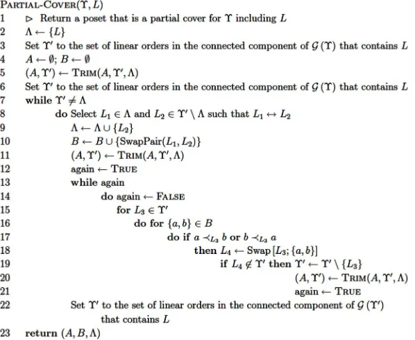
Figure 2 contains pseudocode for the algorithm Partial- Cover
,L
. It works by adding linear orders from\
to one at a time, while maintaining the re- quired properties for A and B. The subroutine Trim in Figure 3 is used to ensure that the required property for
A is maintained. The addition of a linear order to (Step 9) can add at most one new unordered pair to B (Step 10).
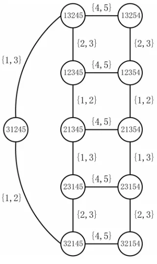
We illustrate the algorithm with the example having
12345, 21345, 23145,32145,31245,13245 12354, 21354, 23154,32154,13254
and L12345. Figure 4 contains the swap graph. The call to Trim in Step 5 finds that 12435 is not in
, so any linear orders in for which 4 is less than 3 should be deleted. In this case, there is no such linear order in . After Step 6, A
3, 4
and B .The first time that Step 8 is executed in Partial-Cover,
1 12345
L and L221345. (There are three choices
for L2. This is just one of them.) Then
12345, 21345
(Step 9) and B
1, 2
(Step 10).The call to Trim in Step 11 finds that 21435 is not in
. The resulting cover relation
3, 4 is not new, soA remains A
3, 4
. The while loop from Steps 13 to 21 has only the swap pair
1, 2 to work with. Linearorder 32154 is missing its
1, 2 swap partner, 31254. Hence, 32154 is deleted from , which is now
12345, 21345, 23145,32145,31245, 13245,12354, 21354, 23154,13254 .
The second time that Step 8 is executed, L121345 and L2 = 23145. Then
12345, 21345, 23145
(Step9) and B
1, 2 , 1,3
(Step 10). The call to Trim in Step 11 finds that 23415 is not in . The resulting cover relation
1, 4 is new, so A is extended to
1, 4 , 3, 4
A . None of the linear orders in has
4 less than 1, so the call to Trim does not change .
The while loop from Steps 13 to 21 now has the swap
pair
1,3 to work with. Linear order 13254 is miss- ing its
1,3 swap partner, 31254 . Hence, 13254 is deleted from , which is now
12345, 21345, 23145,32145,31245, 13245,12354, 21354, 23154 .
The third time that Step 8 is executed, L121345 and L221354. Then
12345, 21345, 23145, 21354
(Step 9) and
1, 2 , 1,3 , 4,5
B (Step 10). The call to Trim in
Step 11 finds that 21534 is not in . The resulting cover relation
3,5 is new, so A is extended to
1, 4 , 3, 4 , 3,5
A . None of the linear orders in
has 5 less than 3, so the call to Trim does not change
. The while loop from Steps 13 to 21 now has the
[image:7.595.149.448.470.715.2]swap pair
4,5 to work with. Linear orders 32145, 31245, and 13245 are missing their
4,5 swap part-Figure 3. Pseudocode for trim
A, ,
.Figure 4. Swap graph for example.
ners. Hence, they are deleted from , which is now
12345, 21345, 23145,12354, 21354, 23154 .
The fourth time that Step 8 is executed, L121354 and L212354. Then
12345, 21345, 23145, 21354,12354
(Step 9) and
1, 2 , 1,3 , 4,5
B (Step 10). The call to Trim in
Step 11 finds that 13254 and 12534 are not in . The resulting cover relations are
2,3 and
3,5 , soA is extended to A
1, 4 , 2,3 , 3, 4 , 3,5
. None of the linear orders in has 3 less than 2, so the call to Trim does not change . The while loop from Steps 13 to 21 has no new swap pairs to work with. Hence, thereare no further linear orders to delete from , which remains
12345, 21345, 23145,12354, 21354, 23154 .
The fifth and last time that Step 8 is executed,
1 21354
L and L223154. Then
12345, 21345, 23145, 21354,12354
(Step 9) and
1, 2 , 1,3 , 4,5
B (Step 10). The call to Trim in
Step 11 finds that 32154 and 23514 are not in . The resulting cover relations are
2,3 , which is not new, and
1,5 , which is new, so A is extended to
1, 4 , 1,5 , 2,3 , 3, 4 , 3,5
A . None of the linear
orders in has 3 less than 2 or 5 less than 1, so the call to Trim does not change . The while loop from Steps 13 to 21 has no new swap pairs to work with. Hence, there are no further linear orders to delete from
, which remains
12345, 21345, 23145,12354, 21354, 23154 .
At this point, .
The resulting poset P has the cover relations in A, namely, 1P4,1P5, 2P3,3P4, and 3P5. The
set of linear extensions of P is exactly the final value of , namely,
12345, 21345, 23145,12354, 21354, 23154
.5.3. Proof of Correctness
We assume that the following loop invariants hold each time that the test at the top of the while loop body (Step 7) is executed.
1) L .
2)
is a connected graph, and
is a con- nected graph.3) The directed graph
X A,
contains no cycles. 4) Every element of is a linear extension of
Min A , that is,
Min
A
.5) The set A equals the set of ordered pairs
a b, X X for which there exists L such that
SwapL a b; , .
6) Min
A Down
B and consequently
Up A Down B .
7) The set B equals the set of unordered pairs
a b, X such that a b and such that there exist ,L L satisfying SwapPair
L L ,
a b, .8) Let Q L L 0, , ,1 Lk be a B -labeled path of
linear orders such that L0 ,aL0 b, and aLk b
and such that Q is a shortest B-labeled path from L0
to Lk . Let Q L L0, , ,1 Lk be the
a b, -mirrorpath for Q. Then, all of the Li's are in , and either
all of the Li’s are in or none of them are.
Together, these invariants suffice to demonstrate the correctness of Partial-Cover, culminating in Theorem 11.
[image:8.595.93.253.286.555.2]5.
Invariant 2 is guaranteed by Steps 6 and 22 and by the way that linear orders are selected for addition to (Step 8).
Invariants 1 and 2 guarantee that, whenever Step 8 is reached, there is a suitable L L1, 2 pair to select.
The fact that is guaranteed through the initi- alization in Step 3 and the fact that any change to
always selects a subset of .
Initialization. After initialization (Steps 2 through 6), all invariants are true for the first execution of Step 7, for the following reasons. We have
L and B . The execution of Trim (Step 5) ensures that Invariants 4 and 5 hold, while maintaining L (Invariant 1). Step 6 guarantees Invariant 2. Invariant 3 holds because the only order relations in A are cover relations in L. The fact that B makes Invariants 6, 7, and 8 true vacuously.Execution of the loop body. The fact that
requires that the algorithm never deletes an element of from in Step 19 or in Trim. That fact also im- plies L , since L is initially put in (Step 2) and could only be deleted in Step 19 or in Trim.
The algorithm never deletes an element of from
in Trim. To obtain a contradiction, assume that
j
L is deleted in Step 12 of Trim and that it is the first element of deleted. The deletion of Lj is caused by a sequence a c c 1, , ,2 ckb such that
1
2 i, i
k ,c c A, for 1 i k 1, and bLj a. For
each i satisfying 1 i k 1, there exists an ˆLi
such that ciLˆi ci1, and SwapL c cˆi;
i, i1
. Thereis a path in
from Lj to ˆLi that does not con-tain an edge with swap pair
c ci, i1
, since
c ci, i1
B contradicts
c ci, i1
A . Consequently,i
c and ci1 are in the same order in ˆLi and in Lj,
which implies that ciLj ci1. Taken together, these
relations imply that aLj b, a contradiction to bLj a.
We conclude that Lj is, in fact, not deleted in Trim. The algorithm never deletes an element of from
in Step 19. The deletion of an element L3
depends on the swap pairs in B. More particularly, such a deletion would require a B-labeled path in
labeled from B from L3 to some L4 that has a swap
pair from B that goes to a linear order outside . This cannot happen because of Invariant 8. We conclude that L3 is, in fact, not deleted in Step 19.
Invariant 3 is maintained because the existence of a cycle in A implies that A and B are inconsistent.
Invariants 4 and 5 are maintained by Trim.
The consistency of A and B (Invariant 6) is maintained by Trim and the loop at Steps 15 through 21.
Invariant 7 is maintained by the way that elements are added to B (Step 10).
It remains to show that Invariant 8 holds; this is demonstrated in the following lemma.
Lemma 10 Each time that Step 8 is about to be
executed, Invariant 8 holds.
Proof. Let P L L 0, , ,1 Lk be a B-labeled path of
linear orders such that L0 , aL0 b, and aLk b
and such that P is a shortest B-labeled path from L0
to Lk . Let P L L0, , ,1 Lk be the
a b, -mirrorpath for P.
To obtain a contradiction, assume that there is some
i
L that is not in . Let Li be the first such. Then
0
i , so Li1 . Let
c d, SwapPair
Li1,Li
B.Since Li , Li1 cannot be in , since it would
have been deleted in a previous iteration due to the swap pair
c d, being in B. This is a contradiction. We conclude that all of the Li’s are in .We next show that P is not just a shortest B-
labeled path but is also a shortest path in
. Let
, <L0 and <Lk
C c d c d d c . For any path from L0
to Lk in
, every
c d, C must be theswap pair for some edge in the path. Consequently, CB. Moreover, there is a path in
that uses swap pairs only from C and each only once, so the length of every shortest path from L0 to Lk is C .(Think about the swaps done by bubble sort; these give one such shortest path.) Since P is a shortest B - labeled path from L0 to Lk, it must be a C-labeled
path having kC . Note that, therefore, no swap pair occurs more than once in P.
We next show that P is a B-labeled path. Since
P contains no swap pair more than once and since
0 L
a b and aLk b, if there is a swap pair
a x, labeling an edge of P, we must also have the swap pair
b x, labeling another edge of P, and vice versa. More succinctly,
a x, C if and only if
b x, C. Let
c d, SwapPair
L Li, i1
, for some i satisfying0 i k 1. If
c d, a b, , then
c d, SwapPair
L Li, i1
. If
c d, a d, , then
b d, SwapPair
L Li, i1
, which is in C by theargument above. Similarly, if
c d, b d, , then
a d, SwapPair
L Li, i1
, which is in C by theargument above. We conclude that P is a C-labeled path and hence a B-labeled path.
Finally, we show that either all of the Li’s are in
or none of them are. To obtain a contradiction, suppose that Li and that Li1 , for some i satisfying
0 i k 1. (The case Li and Li1 will
yield a contradiction by an analogous argument.) But, in this case, Li would have been deleted from in an
earlier iteration, a contradiction. From this contradiction, we conclude that either all of the Li’s are in or
Hence, Invariant 8 holds.
The correctness and time complexity of the algorithm are now in view.
Theorem 11 Algorithm Partial-Cover
,L
returns aset A such that Min
A is a partial cover of including L . The algorithm has time complexity
2 2
O n .
Proof. The correctness of the algorithm follows from
the prior discussion of the loop invariants. For the time complexity, we first note that
2A O n and B O n
2 .We examine the subroutine Trim. Trim is executed once in Step 5; once for each addition to (Step 11;
O times in total); and once for each deletion in
Step 19 (Step 20; O
times in total). Hence, Trim is executed O
times. The loop in Steps 5 through 9 requires O n
time for one execution. The time complexity to test coverage in Step 11 requires
2O A O n time. Hence, the loop in Steps 10
through 13 requires O n
2
time for one execution.The while loop is executed O
times, since eachadditional iteration of the loop because done False
requires the reduction of the cardinality of by at least one. We conclude that the total time spent in trim is
2 2
O n .
It is easy to check that the complexity bound for all calls to Trim dominates the time complexity of the algorithm. Hence, the time complexity of Partial-Cover is
2 2
O n , as required.
REFERENCES
[1] B. S. Baker and E. G. Coffman, “Mutual Exclusion Sche- duling,” Theoretical Computer Science, Vol. 162, No. 2,
1996, pp. 225-2
[2] P. Barcia and J. O. Cerdeira, “The k-Track Assignment Problem on Partial Orders,” Journal of Scheduling, Vol. 8, No. 2, 2005, pp. 135-143.
[3] F. A. Chudak and D. B. Shmoys, “Approximation Algo- rithms for Precedence-Constrained Scheduling Problems on Parallel Machines That Run at Different Speeds,”
Journal of Algorithms, Vol. 30, No. 2, 1999, pp. 323-343.
[4] J. R. Correa and A. S. Schulz, “Single-Machine Schedul- ing with Precedence Constraints,” Mathematics of Opera- tions Research, Vol. 30, No. 4, 2005, pp. 1005-1021.
[5] T. Kis, “Job-Shop Scheduling with Processing Alterna- tives,” European Journal of Operational Research, Vol. 151, No. 2, 2003, pp. 307-332.
[6] M. Peter and G. Wambach, “n-Extendible Posets, and How to Minimize Total Weighted Completion Time,” Discrete Applied Mathematics, Vol. 99, No. 1-3, 2000, pp. 157-
[7] N. Policella, A. Oddi, S. F. Smith and A. Cesta, “Gener- ating Robust Partial Order Schedules,” Proceedings of Principles and Practice of Constraint Programming,Vol. 3258, 2004, pp. 496-511.
[8] D. B. Shmoys, C. Stein and J. Wein, “Improved Approxi- mation Algorithms for Shop Scheduling Problems,” SIAM Journal on Computing, Vol. 23, No. 3, 1994, pp. 617-
[9] C. Grasso and C. Lee, “Combining Partial Order Align- ment and Progressive Multiple Sequence Alignment In- creases Alignment Speed and Scalability to Very Large Alignment Problems,” Bioinformatics, Vol. 20, No. 10,
2004, pp. 1546-
[10] S. K. Kannan and T. J. Warnow, “Tree Reconstruction from Partial Orders,” SIAM Journal on Computing, Vol. 24, No. 3, 1995, pp. 511-519.
[11] S. Karlin and I. Ladunga, “Comparisons of Eukaryotic Genomic Sequences,” Proceedings of the National Acad- emy of Sciences of the United States of America, Vol. 91, No. 26, 1994, pp. 12832-12836.
[12] K. Miyakawa and H. Narushima, “Lattice-Theoretic Pro- perties of MPR-Posets in Phylogeny,” Discrete Applied Mathematics, Vol. 134, No. 1-3, 2004, pp. 169-192.
[13] P. L. Hammer, A. Kogan and M. A. Lejeune, “Modeling Country Risk Ratings Using Partial Orders,” European Journal of Operational Research, Vol. 175, No. 2, 2006,
pp. 836-859
[14] S. Holland and W. Kiessling, “User Preference Mining Techniques for Personalized Applications,” Wirtschaft- sinformatik, Vol. 46, No. 6, 2004, pp. 439-445.
[15] S. Holland, M. Ester and W. Kiessling, “Preference Min- ing: A Novel Approach on Mining User Preferences for Personalized Applications,” Proceedings of Knowledge Discovery in Databases: PKDD 2003, Vol. 2838, 2003, pp. 204-216.
[16] H. Mannila, H. Toivonen and A. I. Verkamo, “Discovery of Frequent Episodes in Event Sequences,” Data Mining and Knowledge Discovery, Vol. 1, No. 3, 1997, pp. 259-
[17] J. Pei, H. X. Wang, J. Liu, K. Wang, J. Y. Wang, and P. S. Yu, “Discovering Frequent Closed Partial Orders from Strings,” IEEE Transactions on Knowledge and Data En- gineering, Vol. 18, No. 11, 2006, pp. 1467-1481.
[18] B. Bollobas and G. Brightwell, “The Structure of Random Graph Orders,” SIAM Journal on Discrete Mathematics, Vol. 10, No. 2, 1997, pp. 318-335.
Vol. 12, No. 3, 1999, pp. 360-373.
[20] S. Felsner and W. T. Trotter, “Posets and Planar Graphs,”
Journal of Graph Theory, Vol. 49, No. 4, 2005, pp. 273-
284.
[21] P. C. Fishburn, P. J. Tanenbaum and A. N. Trenk, “Linear Discrepancy and Bandwidth,” Order, Vol. 18, No. 3,
2001, pp. 237-2
[22] L. S. Heath and S. V. Pemmaraju, “Stack and Queue Lay- outs of Posets,” SIAM Journal on Discrete Mathematics, Vol. 10, No. 4, 1997, pp. 599-625.
[23] M. Naatz, “The Graph of Linear Extensions Revisited,”
SIAM Journal on Discrete Mathematics, Vol. 13, No. 3,
2000, pp. 354-3
[24] G. Agnarsson, S. Felsner and W. T. Trotter, “The Maxi- mum Number of Edges in a Graph of Bounded Dimen- sion, with Applications to Ring Theory,” Discrete Mathe- matics, Vol. 201, No. 1-3, 1999, pp. 5-19.
[25] M. Aguiar and W. F. Santos, “Galois Connections for Incidence Hopf Algebras of Partially Ordered Sets,” Ad- vances in Mathematics, Vol. 151, No. 1, 2000, pp. 71-100.
[26] N. Bergeron and F. Sottile, “Hopf Algebras and Edge- Labeled Posets,” Journal of Algebra, Vol. 216, No. 2,
1999, pp. 641-6
[27] J. Konieczny, “Reduced Idempotents in the Semigroup of Boolean Matrices,” Journal of Symbolic Computation, Vol. 20, No. 4, 1995, pp. 471-482.
[28] F. Ruskey, “Generating Linear Extensions of Posets by Transpositions,” Journal of Combinatorial Theory Series B, Vol. 54, No. 1, 1992, pp. 77-101.
[29] D. B. West, “Generating Linear Extensions by Adjacent Transpositions,” Journal of Combinatorial Theory Series B, Vol. 58, No. 1, 1993, pp. 58-64.
[30] G. Pruesse and F. Ruskey, “Generating Linear Extensions Fast,” SIAM Journal on Computing, Vol. 23, No. 2, 1994,
pp. 373-386
[31] E. R. Canfield and S. G. Williamson, “A Loop-Free Al- gorithm for Generating the Linear Extensions of a Poset,”
Order, Vol. 12, No. 1, 1995, pp. 57-75.
[32] J. F. Korsh and P. S. LaFollette, “Loopless Generation of Linear Extensions of a Poset,” Order, Vol. 19, No. 2,
2002, pp. 115-126.
[33] A. Ono and S. Nakano, “Constant Time Generation of Linear Extensions,” Proceedings ofFundamentals of Com- putational Theory,Vol. 3623, 2005, pp. 445-453. [34] R. Bubley and M. Dyer, “Faster Random Generation of
Linear Extensions,” Discrete Mathematics, Vol. 201, No. 1-3, 1999, pp. 81-88.
[35] P. L. Fernandez, L. S. Heath, N. Ramakrishnan, M. Tan and J. P. C. Vergara, “Mining Posets from Linear Or- ders,” Discrete Mathematics, Algorithms and Applica- tions, 2013, in press.
[36] P. L. Fernandez, L. S. Heath, N. Ramakrishnan and J. P. C. Vergara, “Reconstructing Partial Orders from Linear Extensions,” Proceedings of the Fourth SIGKDD Work- shop on Temporal Data Mining: Network Reconstruction from Dynamic Data, Philadelphia, 20 August 2006, p. 4. [37] A. K. Lee and M. A. Wilson, “A Combinatorial Method
for Analyzing Sequential Firing Patterns Involving an Ar- bitrary Number of Neurons Based on Relative Time Or- der,” Journal of Neurophysiology, Vol. 92, No. 4, 2004,
pp. 2555-2573.
[38] B. A. Davey and H. A. Priestley, “Introduction to Lattices and Order,” 2nd Edition, Cambridge University Press,
Cambridge, 200
[39] G. Brightwell and P. Winkler, “Counting Linear Exten- sions,” Order, Vol. 8, No. 3, 1991, pp. 225-242.
[40] M. R. Garey, D. S. Johnson and L. Stockmeyer, “Some Simplified NP-Complete Graph problems,” Theoretical Computer Science, Vol. 1, No. 3, 1976, pp. 237-267.