Munich Personal RePEc Archive
A single-item continuous double auction
game
Ruijgrok, Matthijs
Utrecht University, Mathematics department
19 October 2012
Online at
https://mpra.ub.uni-muenchen.de/42086/
A single-item continuous double
auction game
M. Ruijgrok
Mathematics Department, Utrecht University.
e-mail: [email protected]
October 19, 2012
A double auction game with an infinite number of buyers and sellers is introduced. All sellers posses one unit of a good, all buyers desire to buy one unit. Each seller and each buyer has a private valuation of the good. The distribution of the valuations define supply and demand functions. One unit of the good is auctioned. At successive, discrete time instances, a player is randomly selected to make a bid (buyer) or an ask (seller). When the maximum of the bids becomes larger than the minimum of the asks, a trans-action occurs and the auction is closed. The players have to choose the value of their bid or ask before the auction starts and use this value when they are selected. Assuming that the supply and demand functions are known, expected profits as functions of the strategies are derived, as well as expected transaction prices. It is shown that for linear supply and demand functions, there exists at most one Bayesian Nash equilibrium. Competitive behaviour is not an equilibrium of the game. For linear supply and demand functions, the sum of the expected profit of the sellers and the buyers is the same for the Bayesian Nash equilibrium and the market where players behave compet-itively. Connections are made with the ZI-C traders model and thek-double auction.
JEL classification: C72, D44
KEYWORDS: Continuous double auction; supply and demand; Bayesian Nash equilib-rium; ZI-C model; k-double auction.
1. Introduction
this type. Second, it provides a simple but effective model of a decentralized competitive market for one good.
Practically all studies on CDA’s are either experimental or involve computer simulations. Theoretical results are lacking because of the complex nature of the CDA. In this paper, we consider an auction of a single item, where sellers and buyers all have some private valuation of this item. The auction participants are chosen successively and randomly to submit a bid (buyers) or an ask (sellers). Once the highest bid becomes equal or larger than the lowest ask, a transaction occurs and the auction is over. The profits for the participants involved in the transaction are equal to the difference between the transaction price and their private valuation.
Before the auction starts, each participant has to choose the value of the bid or ask he or she will make when selected, and this value cannot be changed during the auction. A buyer is therefore confronted with a strategic choice: a high bid will increase his chance of winning the item, but decrease the profit he may gain, and similarly for a seller. This paper will show that the payoff structure of this game is relatively simple. Moreover, for a large class of distributions of the private valuations, there exists a unique Bayesian Nash equilibrium, which can even be explicitly calculated. It will also be shown that the expected profits in this equilibrium have a remarkable property.
The study of the single-item CDA is intended as a first step in a theoretical analysis of the complete CDA, by which is meant an auction where, after the first item is auc-tioned, the successful buyer and seller leave the market and a new item is auctioned. This process then repeats until no more transactions are possible. Parsons (2006) quotes a number of authors who are pessimistic about the possibility of a theoretical analysis of the complete CDA. The results of this paper show that such pessimism is perhaps premature.
The distribution of the private valuations, which can be considered as maximal buying prices for the buyers and minimal selling prices for the sellers, define supply and demand functions and a corresponding competitive equilibrium price. Laboratory experiments, pioneered by Smith (1962), where complete CDA’s were repeated a number of times, have shown that after a short learning period a market price emerges. Moreover, this price converges to the competitive equilibrium price, even though the subjects involved in the experiment were only aware of their own valuations. This finding is very robust and has been replicated many times, see Davis and Holt (1992), chapter 3.
It’s not even necessary to be human to discover the equilibrium price in such repeated CDA’s, as work inspired by the ZI-traders of Gode and Sunder (1993) has shown. Al-though Gode and Sunder were mainly interested in how the structure of a market in-fluences its efficiency, their framework was later adopted by Cliff and Bruten (1997) to show that the price of the good in repeated CDA’s populated by agents with a mini-mal learning capability generally converge to the competitive equilibrium price. These papers are at the origin of what has become a vast literature, of which Anufriev et. al. (2011) and Fano, LiCalzi and Pellizzari (2011) are recent examples.
is auctioned, since the successful traders leave the auction. The game presented in this paper, already interesting in its own right, can therefore be seen as a building block of a game-theoretic model of a complete CDA. An evolutionary version of such a model could serve as a theoretical foundation for Smith’s results and more generally for the emergence of competitive equilibrium in a decentralized market.
Most of the theoretical work on double auctions deals with call markets, see for instance Reny and Perry (2006). The type of model that comes closest to the one presented in this paper is that of the two-player k-double auction introduced by Chatterjee and Samuelson (1983). Although this auction involves only two participants, it can be refor-mulated as an auction with large, in fact infinite, sets of buyers and sellers. This set-up resembles our model of the single-item CDA, in particular in the form of the payoff functions.
To find a Bayesian Nash equilibrium (BNE) of either the k-double auction or the CDA, the expression for the expected payoff to a buyer or seller who adopts a certain strategy, given the strategies of all other auction participants, has to be derived. For thek-double auction this is much simpler than for the single-unit CDA. Satterthwaite and Williams (1989) show that thek-double auction generally has many BNE. In particular, it has a a two-parameter family of such equilibria. Using methods similar to the ones used by Sat-terthwaite and Williams, we will show that in contrast, the single-unit CDA has either no BNE, or a unique one. Moreover, for linear supply and demand functions, an exact expression for the BNE (if it exists) can be given for the single-unit CDA, whereas such an expression is only known for one special case of the k-double auction. Surprisingly, for this special case, when both maximum bidding prices and minimum selling prices are uniformly distributed on the interval [0,1], these expressions are equal when k = 1/2. For the case of linear supply and demand functions, the expected profits for the buyers and sellers can be explicitly calculated. We compare these to the case that the market participants use a strategy corresponding to competitive equilibrium. This means that those who can afford it, bid or ask the competitive equilibrium price and others bid or ask what they want. We will show that this competitive strategy is not an equilibrium, but it still serves as a benchmark. We will show that the sum of the expected profits of the buyers and the sellers in the case of the BNE is equal to that in the case of the competitive strategy. However, the profit in the case of the BNE is spread out over a larger fraction of the population.
Finally, a bonus of this model is that it is possible to slightly adapt it so that it can be applied to the ZI-C model of Gode and Sunder. In this model, rather than choosing a unique value for their bid or ask, players select a random value constrained by their private valuation, when chosen. In particular, we derive an expression for the price dis-tribution of the first transaction in the ZI-C model, a subject on which there has been some discussion, see Jahnsson (2011).
In section 6 an explicit expression for the BNE is given and a connection is made with the k-double auction. In section 7 it is shown that the competitive strategy is not an equilibrium. In section 8, the sum of the expected profits of buyers and sellers in the competitive strategy and the BNE are compared, again in the case of linear supply and demand functions. Section 9 concludes.
2. The model
In this auction, one unit of a certain good will be sold. The set of buyers is identified with the interval [0,1], as is the set of sellers. Each buyer has a maximum price in the interval [0, a], which he is willing to pay for the unit and each seller a minimum price in the interval [0, b] for which she is willing to sell. Without loss of generality, we may assumea=b = 1. These maximum and minimum prices define the type of the trader. The assumption that the number of buyers and sellers and the number of types is (uncountably) infinite is meant as an approximation of the situation where these numbers are large but finite. It is straightforward to derive a finite model by replacing integrals in the payoff functions with finite sums. However, the results on the existence and the explicit expressions for the Bayesian Nash equilibria in the continuous model rely on solving differential equations, which is harder to translate to the finite case. Whether the results reported in this paper continue to hold for finite models will require a separate study.
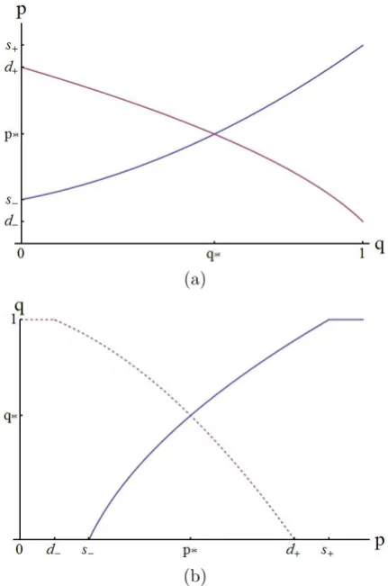
The distributions of the seller and buyer types are common knowledge and follow from the supply and demand functions. For the buyers, we are given a strictly decreasing continuously differentiable demand functionD: [0,1]→[d−, d+], with 0 ≤d−< d+ ≤1.
If p = D(q), then a fraction q of the buyers is willing to pay a price p or less for the unit. The supply side of the market is given by a strictly increasing and continuously differentiable supply function S : [0,1] → [s−, s+], with 0 ≤s− < s+ ≤ 1. If p =S(q),
then a fraction q of the sellers is willing to sell for a price p or more for the unit. We assume that d+ > s− and s+ > d−, to guarantee that the graphs of the supply and
demand functions intersect.
The inverses of the supply and demand function, S−1(m) and D−1(M), can be used
to define the cumulative distribution functions of the types, see Figure 1. If a seller is randomly chosen, then the probability that her type is less or equal to m ∈ [s−, s+] is
S−1(m). If m < s−, this probability is zero and if m > s
+, it is equal to one. The
probability density for the seller types is therefore given by
σ(m) =
(
d dmS
−1(m), if m∈(s
−, s+)
0, if m6∈(s−, s+)
, (1)
(a)
(b)
Figure 1: (a) The supply and demand functions.
(b) S−1(p) (solid line) and D−1(p) (dashed line).
is one. The probability density for the buyer types is therefore given by
µ(M) =
(
d dM(−D
−1(M)), if M ∈(d
−, d+)
0, if M 6∈(d−, d+)
, (2)
At consecutive times τ = 1, τ = 2, . . ., a trader is randomly and uniformly chosen. We can assume that the probabilities of choosing a buyer or a seller are equal. If, say, the fraction of buyers is larger than the fraction of sellers, then a certain amount of ’dummy’ sellers with a minimum selling price of one can be added to even out the ratio of sellers to buyers. When sellers outnumber buyers, extra ’dummy’ buyers with maximum buying price zero can be introduced.
[image:6.595.189.405.72.398.2]to this minimum, with now the buyer as price-taker and the seller as price-maker. To replace the holder of the current minimum ask, a new ask must be strictly smaller. A similar rule applies to buyers.
The strategy of a buyer of type M is the bid x ∈ [0,1] he will offer, when given the opportunity. We assume that all traders with the same type, use the same strategy. The set of strategies of the buyers can therefore be described by a single functionb(M), known as thestrategy profile, where b: [d−, d+]→[0,1]. The strategies of the sellers are
encapsulated by the strategy profilea : [s−, s+] → [0,1], so that a seller of type m will
aska(m).
We will assume that the minimum ask is strictly smaller than the maximum bid, so that the probability that the auction ends in finite time is equal to one.
We define theoutcomeof the transaction as the triple{M, m, t}, whereM ∈[d−, d+] and
m∈[s−, s+] are the types of the buyer and seller involved, and t∈[0,1] the transaction
price. From the outcome, we can calculate the profits of the traders involved, namely
M−t for the buyer and t−m for the seller.
The outcome is a random variable, with a probability distribution that depends on the strategies used by the traders and on the distribution of the types of buyers and sellers. In particular we define
β(M, m, t;x, a(.), b(.)) (3) as the probability density of the event that a buyer of typeM and a seller of typem are involved in a transaction with transaction price t, given that the buyer uses strategy x
and the other buyers play b(M) and the sellers a(m). Givenβ(M, m, t;x, a(.), b(.)), we define:
πb(x, M;a(.), b(.)) =
1
µ(M)
Z s+
s−
Z 1
0
(M −t)β(M, m, t;x, a(m), b(M)) dt
dm . (4)
The functionπb(x, M;a(.), b(.)), which we will often abbreviate asπb(x, M), is the
prob-ability density for the expected payoff of a buyer of typeM who plays strategy x, given that the rest of the buyers play b(M) and the sellers a(m). It means that the expected payoff to the group of buyers whose types are in some interval S ⊂[0,1] is given by
Z
S
µ(M)πb(x, M) dM ,
assuming they all use the strategyx. Similarly,
α(M, m, t;x, a(.), b(.)) (5) is the probability density of the event that a buyer with limitM and a seller with limitm
are involved in a transaction with transaction pricet, given that the seller uses strategy
define
πa(x, m;a(.), b(.)) =
1
σ(m)
Z d+
d−
Z 1
0
(t−m)α(M, m, t;x, a(m), b(M)) dt
dM . (6)
The above expression is often abbreviated as πa(x, m).
It will be shown that πb(x, M) and πa(x, m) are continuous functions of M and m,
re-spectively. Therefore, the a-priori probability that a specific buyer or seller is involved in a transaction is zero, and so the expected profit of every trader is also zero. Never-theless, we will take πb(x, M) and πa(x, m) as the payoff functions for types M and m,
respectively, and assume that the buyer of type M will try to maximize πb(x, M) as a
function ofx, and similarly a seller of type m will want to maximize πa(x, m).
This can be justified in the following way. Consider a model with a finite number of types M1, M2, . . . MN, and a finite number K of buyers and let fi be the number of
buyers of type Mi. Then we can approximate the profit of all the types Mi =i/N by
Z Mi+1/N
Mi
µ(M)πb(x, M) dM ≈
µ(Mi)
N πb(x, Mi)≈ fi
Kπb(x, Mi).
The profit for an individual buyer of typeM is then approximately πb(x, Mi)/K and it
is rational for him to maximize this expression. Since we can consider the model as the limit N, K → ∞ of a finite model, the only consistent choice for a payoff function for the buyers isπb(x, M). The payoff function for the sellers is taken to be πa(x, m).
We define a Bayesian Nash equilibrium of this game as a pair of strategy profiles (a∗(m), b∗(M)) such that y =a∗(m) maximizes π
a(y, m;a∗(.), b∗(.)) for all m ∈ [s−, s+]
and x=b∗(M) maximizes π
b(x, M;a∗(.), b∗(.)) for all M ∈[d−, d+].
3. Expected payoffs
The ingredients that are still missing are expressions forπb(x, M) and πa(x, m). These
will be constructed in a few steps.
We will take the standing maximum bid before τ = 1 to be zero, and the minimum ask at that time to be one and also note that the probability that a transaction occurs at
τ = 1 is equal to zero.
of notation:
β(M, m, t;x, a(.), b(.)) = ∞
X
n=2
P r(no transaction atτ =n−1 and holder maximum bid is of typeM)
P r(seller of typemis chosen)P r(a(m)≤x)P r(t=x) + ∞
X
n=2
P r(no transaction atτ =n−1 and holder minimum ask is of typem)
P r(buyer of typeM is chosen)P r(a(m)≤x)P r(t=a(m)). (7) Note that the events (a(m)≤x), (t=x) and (t=a(m)) are not chance events, so their probabilities are degenerate.
In Appendix A it is shown that a closed expression exists for (7), in terms of the cumu-lative distribution function of the asks:
A(x) = P r(ask≤x) =
Z s+
s−
θ(x−a(m))σ(m) dm , (8)
and the bids
B(x) = P r(bid≤x) =
Z d+
d−
θ(x−b(M))µ(M) dM , (9)
whereθ(z) is defined asθ(z) = 0 if z <0 and θ(z) = 1 if z ≥0. We also define
A(x) =P r(ask< x)
B(x) =P r(bid< x). (10) Then
α(M, m, t;x, a(m), b(M)) =
µ(M)σ(m)θ(b(M)−x) (γ2(x)δ(t−x) +γ1(b(M))δ(t−b(M))) , (11)
and
β(M, m, t;x, a(m), b(M)) =
µ(M)σ(m)θ(x−a(m)) (γ1(x)δ(t−x) +γ2(a(m))δ(t−a(m))) . (12)
Here, the functions γ1(x) and γ2(x) are defined as:
γ1(x) =
1
and
γ2(x) =
1
(1− B(x) +A(x))(1− B(x) +A(x)). (14) Momentarily disregarding the difference between probability and probability density, we can interpret (12) as follows. The probability that a buyer of type M, playing strategy
x, is involved in a transaction with a seller of typem, playing strategya(m) is propor-tional to the probability that a buyer of typeM and a seller of typem are chosen in the process, explaining the term µ(M)σ(m). Also, a necessary condition for a transaction to occur between this buyer and this seller is that x ≥ a(m), which accounts for the term θ(x−a(m)). Finally, the transaction price is either t = x, which happens with a probabilityγ1(x), ort=a(m), which happens with a probabilityγ2(a(m)), thus leading
to the last term. The surprising aspect of (11) and (12) is that the expressions forγ1(x)
and γ2(x) are so simple.
To derive an expression for the expected payoff πb(x, M;a(m), b(M)), we substitute
(12) in (4). This yields
πb(x, M;a(m), b(M)) =
Z s+
s−
Z 1
0
(M −t)σ(m)θ(x−a(m))γ1(x)δ(t−x) dtdm+ Z s+
s−
Z 1
0
(M −t)σ(m)θ(x−a(m))γ2(a(m))δ(t−a(m)) dtdm . (15)
The first part of (15) is easily integrated:
Z s+
s−
Z 1
0
(M −t)σ(m)θ(x−a(m))γ1(x)δ(t−x) dtdm =
A(x)γ1(x)(M−x). (16)
For the second part of (15), we use the following
Lemma 1. Let
1. f(z) : [0,1]→R be a measurable function. 2. g(t) : [a, b]→R be a continuous function.
3. σ(m) : [0,1]→R be a continuous probability density.
Then
Z s+
s−
Z 1
0
g(t)σ(m)f(a(m))δ(t−a(m)) dtdm=
Z 1
0
g(q)f(q) dA(q) (17)
and
Z d+
d−
Z 1
0
g(t)µ(M)f(b(m))δ(t−b(M)) dtdM =
Z 1
0
g(q)f(q) dB(q). (18)
Proof: See Appendix B
Applying equation (17) to f(z) = θ(x−z)γ2(z) and g(t) =M −t, we find: Z s+
s−
Z 1
0
(M −t)σ(m)θ(x−a(m))γ2(a(m))δ(t−a(m)) dtdm = Z 1
0
(M −q)θ(x−q)γ2(q) dA(q). (19)
Substituting (16) and (19) in (15), we finally find the expression for the expected profit of a buyer of type M who plays x, while other buyers play b(M) and the sellers a(m):
πb(x, M;a(.), b(.)) =
(M −x)A(x)γ1(x) + Z x
0
(M −q)γ2(q) dA(q)
. (20)
A similar expression for πa(x, m;a(.), b(.)) can be found:
πa(x, m;a(.), b(.)) =
(x−m)(1− B(x))γ2(x) + Z 1
x
(q−m)γ1(q) dB(q)
. (21)
We note that the expected profit of a buyer has two components. The first one, involving a term M −x corresponds to transactions in which the buyer is the price maker. The second one is an integral over q, involving the term M −q. This term comes from transactions where the buyer is the price taker.
4. Distribution of transaction prices and connection
with ZI-C traders
Apart from giving expressions for expected profits, equations (11) and (12) can also be used to derive the probability distribution of the transaction prices, in case the strategy profiles are continuous, differentiable and strictly increasing. Then A(t) = A(t) and
B(t) = B(t) are also continuous, differentiable and strictly increasing on [s−, s+] and
[d−, d+], respectively. Also, γ1(t) = γ2(t)= (1−B(t) +A(t))−2 for all t∈[0,1].
Figure 2: Distribution of transaction prices for the caseD(x) = 0.55−0.05xandS(x) = 0.1 + 0.7x. The histogram shows the result of a numerical simulation with 50000 transactions, the solid line is the plot of the right-hand side of (22). The average transaction price is ¯T = 0.438, while the competitive price is
p∗ = 0.52.
T(t) = P r(transactionprice ≤t) be the cumulative distribution function of the trans-action prices. Then it is shown in Appendix C that
T(t) = A(t)
(1−B(t) +A(t)). (22) The above result is also relevant for the Zero Intelligence Constrained model of Gode and Sunder (1993). The set-up of this model is similar to that of the game defined in this paper. However, the ZI-C players play a random strategy, where buyers offer a price which is randomly and uniformly chosen between zero and the players type and sellers randomly and uniformly choose a bid between their type and one. Another difference is that there is only a finite number of traders, who leave the market after a successful transaction.
Since the result (22) and its derivation only depend onA(x) and B(x), it is clear that it can be applied to the ZI-C model, when there is an infinite number of traders and we only consider the first transaction.
Gode and Sunder claim on the basis of simulations that the transaction price converges during one trading session to the equilibrium price, but Cliff and Bruten (1997) contend that this happens only for special supply and demand functions. Jahnson (2011) provides an extensive analysis of this debate, which favours Gode and Sunder.
5. Bayesian Nash equilibria
Let us first note that associated with every Bayesian Nash equilibrium, henceforth BNE, there exist in general many other BNE that are essentially equivalent to it. For every pair of strategy profiles (a(m), b(M)), we can define the extramarginal sellers as those whose ask is higher than the maximum bid. Similarly, we can define extramarginal buyers as those whose bid is smaller than the minimum ask. These extramarginal traders will never be involved in a trade. Consequently, we will focus on the strategies of the other traders, who will be referred to asintramarginal traders.
In this section we will limit ourselves to continuous, differentiable and strictly increasing strategy profiles. For ease of notation, introduce
Bc(x) = 1−B(x) = P r(bid≥x).
We have
A(x) =
0 if 0≤x≤a−
Ra−1(x)
s− σ(m) dm =S
−1(a−1(x)), if a
− ≤x≤a+
1 if a+ ≤x≤1,
(23)
and
Bc(x) =
1 if 0≤x≤b−
Rd+
b−1(x)µ(M) dM =D
−1(b−1(x)), if b
− ≤x≤b+
0 if b+ ≤x≤1,
(24)
where S(x) and D(x) are the supply and demand function, respectively. It follows immediately from the above and the assumptions on a(m), b(M), S(x) and D(x) that
A(x) andBc(x) are strictly increasing and strictly decreasing, respectively and both are
continuously differentiable, except ina± and b±, respectively.
The functionsπa(x;m) andπb(x;M) are therefore differentiable with respect tox, except
ina± and b± where jumps in the derivatives may occur. We find that the derivatives of
πa(x;m) and πb(x;M), where they exist, are given by:
d
dxπa(x;m) =
2(m−x)(−Bc′(x)A(x) +Bc(x)A′(x)) +Bc(x)(Bc(x) +A(x))
(Bc(x) +A(x))−3
d
dxπb(x;M) =
2(M −x)(−B′
c(x)A(x) +Bc(x)A′(x))−A(x)(Bc(x) +A(x))
(Bc(x) +A(x))−3
(25)
Lemma 2. Let a : [s−, s+] → [0,1] and b : [d−, d+] → [0,1] be continuous and strictly increasing and let y = a(m) maximize πa(y, m;b(.), a(.)) for all m ∈ [s−, s+] and x =
b(M)maximizeπb(x, M;b(.), a(.))for allM ∈[d−, d+]. Denote a(s±) =a± andb(d±) =
b±. Then
1. a(m)> m, for all m∈[s−, b+) and b(M)< M, for all M ∈(a−, d+]. 2. a−≥d− and b+≤s+.
3. a(b+) =b+ and b(a−) =a−.
4. The set of intramarginal sellers is [s−, b+] and the set of intramarginal buyers is
[a−, d+]. Proof:
1. From (25) it follows that ddxπa(x;m)|x=m = Bc(x)(Bc(x) +A(x)) > 0, for m ∈
[s−, b+). Therefore, πa(y, m) is maximized in a value y = a(m) > m. The proof
that b(M)< M on (a−, d+] is similar.
2. Assume a− < d− and a− < b−. This implies that the ask of the seller of type s− is lower than the smallest possible bid, so this seller is a guaranteed winner, if she is chosen. It is clear that this seller can increase her expected profit by choosing a strategy a′, with a
− < a′ < b−, since she will remain a sure winner, but this time with a higher profit when she is the price-maker and the same profit when she is the price-taker. Therefore, a(m) does not maximize the expected profit of the sellers.
Assume a− < d− and a− ≥ b−. The expected profit for a buyer of type d− is then zero. He can improve this to a positive value by choosing a strategyb′ with
a− < b′ < d−, because then he has a positive probability of being involved in a transaction, when chosen, with a positive profit for him. Thus, b(M) does not maximize the expected profit of the buyers. From this contradiction we conclude that a−≥d−. The proof that b+ ≤s+ is similar.
3. We have that πb(x, M) = 0 for x ≤ a−. Also, because A(x) > 0 for x > a−, we
find from (20) that πb(x, M) >0 for a− < x < M. Combining with part 1 of this lemma, we conclude thata− < b(M)< M, for a− < M < d+. Taking M ↓a− and using continuity ofb(M), it follows that b(a−) =a−. The proof thata(b+) =b+ is
similar.
4. Let m > b+. Since a(m) is strictly increasing, a(m) > a(b+) = b+, therefore
no seller of type larger than b+ will ever participate in a transaction. A similar
argument shows that the intramarginal buyers constitute the set [a−, d+].
(a) (b)
Figure 3: (a) Linear supply and demand functionsS(x) andD(x). (b) The functions a(x) andb(x) corresponding to the BNE.
5.1. First order conditions
To systematically derive BNE of the game, we first note that in (25) we can replace the parameter m by a function of x, on the interval [s−, b+], by using the fact that
x=a(m) on this interval. Therefore, m=a−1(x) =S(A(x)). Similarly, M =D(B
c(x))
on [a−, d+].
The first order conditions for a maximum then become d
dxπa(x;m) = 0 ,
d
dxπb(x;M) = 0.
However, this set of equations is not independent, as is easily seen from (25). Rather, we have one differential equation and one consistency equation:
2(S(A(x))−x)(−B′
c(x)A(x) +Bc(x)A′(x)) +Bc(x)(Bc(x) +A(x)) = 0, (26)
Bc(x)(D(Bc(x))−x) = A(x)(x−S(A(x))),for x∈[a−, b+]. (27)
There are also the following boundary conditions :
A(a−) = 0, Bc(b+) = 0.
The values ofa−andb+are not yet determined. Note that from the boundary conditions
and the consistency equation (27), we have
A(b+) =S−1(b+), Bc(a−) = D−1(a−),
which also follows from Lemma 2.3 and (23) and (24). Also, A(x) must be strictly increasing and Bc(x) strictly decreasing.
A practical way to find the solutions A(x) and Bc(x) and the values of a− and b+ is
to use (27) to express A(x) in terms of Bc(x) (or the other way round) and substitute
in (26). Together with the boundary condition A(a−) = 0, this then yields a solution
A(x;a−), with a− a free parameter. This expression can in turn be used to construct
[image:15.595.86.510.68.211.2]yields a one-parameter family of solutions, parametrized by a−. We will show in the next section that at least for linear supply and demand functions this is not true: in that case the BNE either does not exist or it is unique.
As a preparation, we consider the system (26), (27) from a geometric viewpoint. We introduce a time-like parameterτ and construct a vector fieldF(A, Bc, x) on [0,1]3, such
that the solution curves of the corresponding flow, defined by
d
dτ(A(τ), Bc(τ), x(τ))
t=F(A, B c, x)
are solutions of (26), (27).
We first note that (26) can be interpreted as stating that a certain 1-form vanishes for all (A, Bc, x):
2(S(A)−x)BcdA−2(S(A)−x)A dBc+Bc(Bc+A)dx= 0. (28)
The solution curve of the flow through a point (A, Bc, x) has tangent vector (dA, dBc, dx),
which according to (28) lies in a plane tangent to:
v
1 = (2(S(A)−x)Bc,−2(S(A)−x)A, Bc(Bc+A))t.
Secondly, the consistency condition (27) defines a surfaceV in (A, Bc, x) space, to which
the solutions are confined. If we write (27) in the formf(A, Bc, x) = 0, then it follows
that the tangent vector of a solution curve through (A, Bc, x) must lie in a plane tangent
to
v2 =∇f(A, Bc, x).
It then follows that the vector field given by
F(A, Bc, x) =v1×v2 (29)
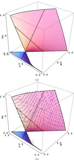
yields solution curves that are solutions to (26), (27), provided the initial condition lies on the planeV. Figure 5 shows the surfaceV and the vector field (29) on it, in the case
S(x) = 0.3 + 0.6x and D(x) = 1−x. As will be shown in the next section, for linear
S(x) and D(x) the vector field has a singular point on V, of saddle type. This saddle point has a stable and an unstable manifold, the separatrices, which are also are shown in Figure 4. From this figure it is clear that the separatrix connecting the planeBc = 0
with the plane A = 0 is the only possible solution curve which fulfils the boundary conditions.
However, it might happen that the separatrix intersects the plane Bc = 0 in a value
x > s+. This would imply that b+ = x > s+, which contradicts Lemma 2.2. In such a
(a)
[image:17.595.169.426.71.625.2](b)
Figure 4: The surface V and the vector field (29) on it, for the case S(x) = 0.3 + 0.6x
and D(x) = 1−x. Here, s+ = 0.9, d− = 0, a− = 0.43 and b+ = 0.78, so that
6. Special case:
S(x)
and
D(x)
linear functions
We now consider the special case that the supply function is given byS(x) = s−+αxand the demand function byD(x) = d+−βx, forx∈[0,1] and construct explicit expressions
for A(x) and Bc(x). This corresponds to the situation that the types of the sellers are
uniformly distributed over the interval [s−, s+] and the types of the buyers uniformly
over [d−, d+].
The system (26), (27) becomes:
2(d+−βBc−x)(−Bc′A+A′Bc)−A(A+Bc) = 0 (30)
Bc(d+−βBc −x) = A(x−s−−αA). (31) It is shown in appendix D that an explicit solution of (30), (31) is given by:
A(x) =
−γα(d+−x) + (2−γ)β(x−s−)
2βα(d+−s−)
(d+−s−+
α(d+−x) +β(x−s−)
2√αβ ), (32)
and
Bc(x) =
(1 +γ)α(d+−x)−(1−γ)β(x−s−)
2βα(d+−s−)
(d+−s−+
α(d+−x) +β(x−s−)
2√αβ ), (33)
with
γ =
√
β
√
α+√β .
To finda−, we solveA(x) = 0 by equating the first factor in (32) to zero and using that
γ2α−(1−γ)2β= 0. This gives
a−=s−+ (1−γ)2(d+−s−). (34)
A similar procedure shows that
b+=d+−γ2(d+−s−). (35)
A(x) andBc(x) have a second root, common to both, but this root is not in the interval
[0,1] and therefore not of interest.
As noted previously, necessary and sufficient conditions for these expressions to corre-spond to a unique BNE are b+ ≤ s+ and a− ≥ d−. These conditions are equivalent with
d+−s−
√ √ ≤
√
α
√ √ , √d+−√s− ≤ √
β
We note that not every pair (α, β) ∈ [0,1]2 yields a supply and demand function that
intersect in a point withx-coordinate between one and zero. It is easy to check that we need α+β ≥d+−s−.
Using the expression forA(x) and (23), we find in the caseα 6=βthe following expression from whicha(m) can easily be recovered:
(α−β) (1−γ)
(a(m)−s−) (d+−s−)
=
α+β+pαβ−(β+ 2pαβ)
s
1− 4 (2√α+√β)2
(α−β) (1−γ)
(m−s−) (d+−s−)
, (37)
and when α=β, we have
a(m) = 2 3m+
1 4d++
1
12s−. (38) In both cases these expressions hold for all s−≤m ≤b+. It is straightforward to check
that, indeed,a(s−) =a− and a(b+) = b+.
Similarly, we have in the case α6=β, (α−β)
γ
(d+−b(M))
(d+−s−)
=
−(α+β+pαβ) + (α+ 2pαβ)
s
1 + 4 (√α+ 2√β)2
(α−β)
γ
(d+−M)
(d+−s−)
, (39)
and when α=β, we have
b(M) = 2 3M +
1 4s−+
1
12d+. (40) In the special case that the types of both sellers and buyers are uniformly distributed over [0,1], so that S(x) = x and D(x) = 1−x, we have
a(m) = 2 3m+
1
4 , 0≤m ≤ 3 4
b(M) = 2 3M +
1 12 ,
1
with transaction price in the case k = 1/2 equal to the average of the bid and the ask. A strategy for a buyer is a function that assigns to each valuation a bid and similarly for the seller. The problem is to find pairs of strategy functions that form a Bayesian Nash equilibrium.
A slightly different interpretation is that there are infinite sets of buyers and sellers. The distribution of their types is given by the commonly known probability density, which now serves as a distribution function. Nature randomly chooses a buyer and a seller from these populations. Traders of the same type will play the same strategy, i.e. the bid they will offer or the ask they will make. After the buyer and seller are chosen, the corresponding bid and ask are compared and if the bid is higher or equal to the ask, there is a transaction with price equal to the average of the ask and the bid. Again, we are looking for Bayesian Nash equilibria.
Chatterjee and Samuelson found that in the case that the valuations are uniformly dis-tributed over the interval [0,1], for both the sellers and the buyers, a Bayesian Nash strategy is given by expression (41), exactly as in this game. This might suggest that the solutions found for this game might also be solutions of thek-double auction, but it is relatively easy to check that this is not the case.
Satterthwaite and Williams (1989) showed that, in contrast to this game, Bayesian Nash equilibria of the k-double auction are generally not unique, but form a two-parameter continuous family of equilibria.
7. One-price strategies
We will define a one-price strategy, with price p, as a strategy such that every buyer of type greater or equal to p will bid p, while every seller of type less or equal to p will ask p. As it is clear that all transactions will happen at a price p, those buyers whose type is below this value are never involved, nor are the sellers with a type greater than
p; they are extramarginal traders.
The strategies of the extramarginal traders are inconsequential, but for simplicity we will restrict them to a.e. continuously differentiable ask- and bid functions. A pair of one-price strategies is therefore given by
a(m) =
(
p, if m ∈[s−, p] ¯
a(m), if m ∈(p, s+]
,
and
b(M) =
(
¯
b(M), if M ∈[d−, p)
p, if M ∈[p, d+]
.
Here ¯a(m) is a continuously differentiable function such that ¯a(m) ≥ m and ¯b(M) is a continuously differentiable function such that ¯b(M)≤M, see Figure 5.
(a) (b)
Figure 5: The strategies a(m) and b(M).
(a) (b)
Figure 6: Cumulative distribution of asks A(x) and A(x).
Assume that p ≥ p∗, with p∗ the competitive price. To this price p there correspond fractionsqd< qs such that S(qd) =p and D(qd) =p. We have that
A(x) = 0, s− ≤x < p , A(p) =qs
A(x) = 0, s− ≤x≤p
B(x) = 1, p≤x < d+
B(x) = 1, p < x≤d+ , B(p) = 1−qd.
The graphs of the above expressions are shown in Figures 6 and 7.
Using (13), (14) and (20), we find for x < p πb(x, M) = 0,
where we have used a shorthand forπb(x, M;a(.), b(.)). Whenx=p, we have
πb(p, M) =
(M −p)qs
(qs+qd)qs
+ (M −p)qs (qs+qd)qd
= M −p
(a) (b)
Figure 7: Cumulative distribution of bids B(x) and B(x).
Finally, for p < x≤d+ we find
πb(x, M) =
M −x A(x) +
(M −p)qs
(qs+qd)qd
+
Z x
p
(M −q) A ′(q
A(q)2 dq
= (M −p)qs (qs+qd)qd
+M −p
A(p) −
Z x
p
1
A(q)dq =k(qs, qd)(M −p)−
Z x
p
1
A(q)dq , with
k(qs, qd) =
q2
s+q2d+qsqd
qsqd(qs+qd)
It is clear thatπb(x, M) is discontinuous in x=p. We have that
k(qs, qd)−
1
qd
= q
2
s+q2d+qsqd
qsqd(qs+qd) −
1
qd
= qd
qs(qs+qd)
>0.
The graph ofπb(x, M) is shown in Figure 8. We conclude from this figure that when all
sellers use strategya(m) and all other buyers use strategy b(M), then for a buyer with limit M > p, it is profitable to play a strategy larger than p. Although there does not exist a unique best reply, there is a whole interval of values of x that lead to a higher profit for this buyer than playing x=p.
Figure 8: Graph of πb(x, M).
It is worth noting that the relative profit jump for buyers
1
M −p(limx↓p πb(x, M)−πb(p, M)) =
qd
qs(qs+qd)
is equal to the relative profit jump for sellers 1
p−m(limx↑p πa(x, m)−πa(p, m)) =
qs
qd(qs+qd)
,
if and only ifqs =qd, i.e. if p=p∗.
8. Comparison of the BNE and competitive behaviour
for linear supply and demand
Many interesting aspects of the BNE can be calculated explicitly in the case of linear supply and demand functions. Here, we will focus on two of these, namely the fraction of intramarginal traders and the sum of the expected profit of the successful seller and buyer, which we will call total expected profit. These will be compared to the case that the players play competitive strategies.
The auction where the players use competitive strategies will be called the competitive market. In this market, every buyer of type greater or equal to p∗ and every seller of type less or equal to p∗ are intramarginal, so for both the populations of buyers and sellers, the fraction of intramarginals is q∗. For linear supply and demand functions
S(x) = s−+αx and D(x) = d+−βx, these values are
p∗ = αd++βs−
α+β =s−+
α(d+−s−)
α+β , q
∗ = d++s−
α+β .
In the case of the BNE, sellers with a limit less or equal to b+ are intramarginal, as are
is larger for the BNE than for the competitive market. This can be seen by noting that
a−=s−+
α(d+−s−)
(√α+√β)2
=s−+
α(d+−s−)
α+β −
α(d+−s−)
α+β +
α(d+−s−)
(√α+√β)2
=p∗+α(d
+−s−)(
1
(√α+√β)2 −
1
α+β)< p
∗.
Similarly, b+ > p∗.
When the sellers and buyers use strategy profilesa(m) andb(M), respectively, the profit density for the sellers is given byπa(x=a(m), m). This means that the fraction of sellers
whose limit is m ∈ [m1, m2] have an expected profit of Rm2
m1 σ(m)πa(x = a(m), m)dm.
Note thatπa(x=a(m), m) also depends on b(M).
The expected payoff for the whole population of sellers is given by
Pa=
Z s+
s−
σ(m)πa(x=a(m), m)dm . (42)
In the case of the competitive market, it follows from the previous section that
πa(x=a(m), m) =
((p∗−m)
q∗ , if m ∈[s−, p ∗] 0, if m ∈(p∗, s
+]
,
so that
Pac =
Z p∗
s−
σ(m)(p∗−m)
q∗ dm = 1
q∗
Z q∗ 0
(p∗−S(x))dx ,
where the last equation results from the substitution x = S−1(m). This expression is
easily calculated:
Pc a =
1 2(p
∗
−s−).
By a similar reasoning we find that the expected profit for the buyers in the competitive market is given by
Pbc = 1
2(d+−p ∗),
so that the total expected profit in the competitive market is
Pc = 1
For the case of the BNE, (42) becomes:
PaBN E =
Z b+
s−
σ(m)
(a(m)−m)Bc(a(m))
(A(a(m)) +Bc(a(m)))2 −
Z 1
a(m)
(q−m) (A(q) +Bc(q))2
B′
c(q)dq
dm
(44)
Because the functions in the above expression are known and relatively simple, this integral can be calculated. In Appendix E, it is shown that, quite surprising, also here
PBN E = 1
2(d+−s−), or in other words:
PBN E =Pc.
9. Conclusion
We have introduced a game which models a simple version of a continuous double auc-tion. The players of the game are either buyers or sellers of one good and each buyer has his own maximum buying price and each seller a minimum selling price. The aggregation of these maxima and minima produce demand and supply functions, respectively, the intersection of which define the competitive equilibrium. The players choose a buying price (buyers) or selling price (sellers) before the start of the game. Then, a unit of the good is auctioned using the continuous time double auction method.
Although this model is a very reduced form of real continuous double auctions, it retains the important feature that in choosing strategies, players have to balance the desire for a high profit with the need to outbid or undersell the competition.
The functions describing the expected payoffs were found to have a quite simple form. Also, the distribution of the expected transaction prices is given by a simple formula, which as a by-product also serves as an expression for the price of the first transaction in Gode and Sunder’s ZI-C model. A further analysis of the payoffs of this game showed that for linear supply and demand functions, there exists either no Bayesian Nash equi-librium within the set of differentiable and strictly increasing strategies, or a unique one, and in the latter case an explicit expression was found.
It was shown that the set of strategies corresponding to a market in competitive equi-librium is not a Bayesian Nash equiequi-librium.
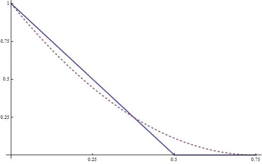
Finally, it was found that the Bayesian Nash solution has a welfare property in common with the competitive market, namely the sum of the expected payoffs for sellers and buy-ers is the same in both markets. This is illustrated in Figure 10, which shows the profit densities for the sellers in the case of the Bayesian Nash equilibrium and the case of the competitive market, for the uniform case where the demand function is D(x) = 1−x
Figure 9: Profit density function πa(x = a(m);m) for the Bayesian Nash equilibrium
(dashed line) and for the competitive strategy (solid line), for S(x) = x and
D(x) = 1−x.
0.25. For the competitive market this is obvious. The first seller chosen with a limit price equal or lower than the competitive pricep∗ = 0.5 is the one involved in the transaction and she will make a profit equal top∗ minus her limit price. Since the limit prices of the sellers are uniformly distributed over [0,1], it is clear that the average profit will be 0.25. The expected profit in the case of the Bayesian Nash equilibrium can be calculated, and due to the symmetry of the supply and demand function the calculation only involves integrating a quadratic function.
There are still many unanswered questions about this game. Are there Bayesian Nash equilibria which are not differentiable and strictly increasing? Does the uniqueness of the Bayesian Nash equilibrium and its welfare property also hold if the supply and demand function are not linear? Can the results be translated to a setting with a finite number of players?
Probably the most important unsolved problem is to give a strategic foundation for competitive equilibrium in the type of double auctions that have been so widely studied since Smith (1962). The next step in this line of research will have to be to expand the game to include multiple rounds, with successful traders exiting the market after each round.
A. Derivation of the distribution of outcomes
To translate (7) into a mathematical expression, we will introduce some notation. Let
Xk denote the stochastic variable defined by the maximum bid at τ = k and Yk the
minimum ask at that time. Let typemaxk be the type of the buyer who holds the
maximum bid at τ = k, and typemink the type of the seller who holds the minimum
ask at that time.
write:
P r(no transaction atτ =n−1 and holder maximum bid is of typeM) dM =
P r(Xn−1 =xandYn−1 > xandtypemaxn−1 =M)dM . (45)
The event (Xn−1 = x, Yn−1 > x, typemaxn−1 = M) can occur in a number of ways,
which we classify according to the number of bids in the sequence ofn−1 shouts made up till timeτ =n−1.
Since Xn−1 =x > 0, it follows that at τ =n−1 at least one bid was made. Let k ≥ 1
be the number of bids in the sequence, then there are n−1−k asks in the sequence, each of which is larger than x. The probability that n−1−k sellers were chosen and that all asks are larger than x is ((1−A(x))/2)n−1−k. There are n−1
n−1−k
= n−k1
ways in which the asks can be distributed over then−1 positions of the sequence.
Of the k bids, one must be made by a buyer of type M, which happens with proba-bility(density) µ(M)dM. The other k−1 bids must either be all smaller than x, or the bids that are equal to x must have been made after the buyer of type M had made his bid. If we consider the sub-sequence of bids, the winning bid can be in position 1, 2,. . .,k. Therefore, the probability(density) that k buyers were selected and that in the subsequence of bids a player of type M was chosen, all buyers before him made a bid smaller thanx and all those after him a bid smaller or equal to x is:
(1 2) k k X l=1
B(x)l−1B(x)k−lµ(M)dM . (46)
Putting the above together, we find:
P r(Xn−1 =xandYn−1 > xandtypemaxn−1 =M)dM =
(1 2)
n−1µ(M)
n−1 X
k=1
n−1
k
(1−A(x))n−1−k
k
X
l=1
B(x)l−1B(x)k−ldM
=un−1(x)µ(M)dM (47)
Expression (47) can be simplified. There are two cases:
1. B(x) =B(x). Then
k
X
l=1
B(x)l−1B(x)k−l =k B(x)k−1.
Since for general v, w∈R,
N X k=1 N k
k vN−kwk−1 =N(v+w)N−1, we find that
un−1(x) =
1
2(n−1)((1−A(x) +B(x))/2)
n−2. (48)
2. B(x)< B(x). Then
k
X
B(x)l−1B(x)k−l=B(x)k−1
k
X
(B(x)
B(x))
= B(x)
k
B(x)− B(x)(1−(
B(x)
B(x))
k). Substitution yields
un−1(x) =
1
B(x)− B(x)
n−1 X
k=1
n−1
k
((1−A(x))/2)n−1−k(B(x)/2)k
−
n−1 X
k=1
n−1
k
((1−A(x))/2)n−1−k(B(x)/2)k
= 1
B(x)− B(x) ((1−A(x) +B(x))/2)
n−1
−
((1−A(x) +B(x))/2)n−1
. (49)
The other factors in (7) have a straightforward expression:
P r(seller with limitmis chosen) dm= 1
2σ(m) dm
P r(a(m)≤x) = θ(x−a(m))
P r(t =x) dt=δ(t−x) dt , (50) with δ(z) the Dirac delta distribution.
Substituting (47) and (50) in the first part of (7), we find:
∞
X
n=2
P r(no transaction atτ =n−1 and holder maximum bid is of typeM)
P r(seller with limitmis chosen)P r(a(m)≤x)P r(t=x)dMdmdt = 1
2 ∞
X
n=2
un−1(x) !
µ(M)σ(m)θ(x−a(m))δ(t−x)dMdmdt =
γ1(x)µ(M)σ(m)θ(x−a(m))δ(t−x)dMdmdt
Again we consider two cases:
1. B(x) =B(x). Then
γ1(x) =
1 4
∞
X
n=2
(n−1)((1−A(x) +B(x))/2)n−2 =
1 4
1
(1−((1−A(x) +B(x))/2))2 =
1
2. B(x)< B(x). Then
γ1(x) =
1 2
∞
X
n=2
1
B(x)− B(x) ((1−A(x) +B(x))/2)
n−1
−
((1−A(x) +B(x))/2)n−1
= 1
2(B(x)− B(x))
1−A(x) +B(x) 1−B(x) +A(x) −
1−A(x) +B(x) 1− B(x) +A(x)
= 1
(1−B(x) +A(x))(1− B(x) +A(x)). (52) In an analogous fashion we find for the second part of (7):
P r(no transaction atτ =n−1 and holder minimum ask is of typem) =
P r(Xn−1 < a(m) andYn−1 =a(m) andtypeminn−1 =m)dm . (53)
Therefore, ∞
X
n=2
P r(no transaction atτ =n−1 and holder minimum ask is of typem)
P r(buyer with limitMis chosen)P r(a(m)≤x)P r(t =a(m)) = ∞
X
n=2
P r(Xn−1 < a(m) andYn−1 =a(m) andtypeminn−1 =m) =
γ2(a(m))µ(M)σ(m)θ(x−a(m))δ(t−a(m))dMdmdt (54)
with
1. A(y) =A(y). Then
γ2(y) =
1
(1− B(y) +A(y))2 . (55)
2. A(y)< A(y). Then
γ2(y) =
1
2(A(y)− A(y))
1− A(y) +B(y) 1− B(y) +A(y) −
1−A(y) +B(y) 1− B(y) +A(y)
= 1
(1− B(y) +A(y))(1− B(y) +A(y)). (56) Putting it al together we find:
β(M, m, t;x, a(m), b(M)) =
µ(M)σ(m)θ(x−a(m)) (γ1(x)δ(t−x) +γ2(a(m))δ(t−a(m))) . (57)
By an analogous reasoning, we find
α(M, m, t;x, a(m), b(M)) =
B. Proof of Lemma 2
LetPσ be the measure on [0,1] which for every measurable set B ⊂[0,1] is defined by:
Pσ(B) =
Z
B
σ(m) dm
Then
A(q) :=
Z s+
s−
θ(q−a(m))σ(m) dm=Pσ({m∈[s−, s+]|q ≥a(m)})
=Pσ(a−1([a−, q])). We find that
Z s+
s−
g(t)σ(m)f(a(m))δ(t−a(m)) dtdm =
Z s+
s−
g(a(m))f(a(m))σ(m) dm
=
Z s+
s−
g(a(m))f(a(m))dPσ(m) (59)
The Transformation lemma for measures (see for instance Halmos [1950], Theorem C, p.163) states that if ν(dx) is a measure on [0,1] and T : R → R is a measurable transformation, then
Z
B
f(T(x))ν(dx) =
Z
T(B)
f(y)νT(dy),
for every measurable B ⊂ [0,1] and every measurable function f : T([0,1]) → R and with νT(C) =ν(T−1(C)) for all measurable sets C ⊂T([0,1]).
Applying the Transformation lemma withT(x) =a(x) to (59), we find
Z s+
s−
g(a(m))f(a(m))dPσ(m) =
Z a+
a−
g(q)f(q)dPσa(q) Since
Pσa([0, q]) = Pσ(a−1([0, q])) =A(q),
we have that
Z a+
a−
g(q)f(q)dPσa(q) =
Z a+
a−
g(q)f(q)dA(q)
=
Z 1
0
g(q)f(q)dPσa(q),
where the last equality follows from the fact thatA(x) = 0 for x≤a− and A(x) = 1 for
x≥a+.
The proof of (18) is similar, using the fact that
Z d+
C. Derivation of the expression for the transaction prices
T(t) =
Z t 0
Z d+
d−
Z s+
s−
β(M, m, t′;x=b(M), a(m), b(M)) dmdMdt′
=
Z t 0
Z d+
d−
Z s+
s−
µ(M)σ(m)θ(b(M)−a(m)) γ(b(M))δ(t′
−b(M)) +γ(a(m))δ(t′
−a(m))
dmdMdt′ =
Z t 0
Z d+
d−
µ(M)γ(b(M))δ(t′−b(M))
Z s+
s−
σ(m)θ(b(M)−a(m))dmdMdt′
+
Z t 0
Z s+
s−
σ(m)γ(a(m))δ(t′−a(m))
Z d+
d−
µ(M)θ(b(M)−a(m))dMdmdt′
=
Z t 0
Z d+
d−
µ(M)γ(b(M))δ(t′−b(M))A(b(M))dMdt′
+
Z t 0
Z s+
s−
σ(m)γ(a(m))δ(t′−a(m))(1−B(a(m))) dmdt′
=
Z 1
0 Z d+
d−
θ(t−t′)µ(M)γ(b(M))δ(t′−b(M))A(b(M))dMdt′
+
Z 1
0 Z s+
s−
θ(t−t′)σ(m)γ(a(m))δ(t′
−a(m))(1−B(a(m))) dmdt′
Applying equation (18) to the first part of the equality and (17) to the second part then yields
T(t) =
Z t 0
γ(t′)(A(t′)B′(t′) + (1−B(t′))A′(t′)) dt′
=
Z t 0
(A(t′)B′(t′) + (1
−B(t′))A′(t′)) (1−B(t′) +A(t′))2 dt
′
=
Z t 0
d dt′
A(t′)
(1−B(t′) +A(t′))dt ′
= A(t)
(1−B(t) +A(t)). (61)
D. Solution for linear supply and demand functions
Recalling the definition
T = A
A+Bc
,
the equation forT becomes:
with T(a−) = 0 and T(b+) = 1. From (31) we find:
(αT2−β(1−T)2)Bc = (1−T)(x−(T s−+ (1−T)d+)). (63)
Note that this equation is satisfied for allBc and T =γ and x= ¯x, with
γ =
√
β
√
α+√β , x¯=γs−+ (1−γ)d+.
The above expression does not constitute a solution of (62), or (30) and (31), as it is only defined inx= ¯x. However, it plays an important role as one of the separatrices of the flow on the surfaceV defined in the previous section.
Rearranging (63), we find:
(T −γ)((α−β)T +γα+ (2−γ)β)Bc = (1−T)(x−x¯+ (T −γ)(d+−s−)), (64)
which yields
d+−βBc−x=
(−x(α−β)−βs−+αd+)T2−β(x−s−)T
αT2−β(1−T)2 . (65)
Substituting (65) in (62), dividing by T and multiplying by αT2−β(1−T)2 yields a
differential equation which we write in the form
f(x, T)dT +g(x, T)dx = 0 (66) with
f(x, T) = 2(α(d+−x)T +β(s−−x)(1−T))
g(x, T) =−αT2+β(1−T)2.
We observe that (66) is exact, i.e.,
∂f ∂x =
∂g ∂T ,
so that (66) can be written in the form
dV(x, T) = 0,
with
We will takecequal to the value V(x, T) has in the point (¯x, γ):
c=V(¯x, γ) = βα
(√α+√β)2(d+−s−).
Equation (67) can be factorized:
V(x, T)−c=
(T −γ)((α(d+−x) +β(x−s−))T +γα(d+−x)−(2−γ)β(x−s−) = 0,
giving two branches which intersect in (¯x, γ) which is therefore a critical point of the flow. These two branches are the separatrices. As noted,T =γ does not yield a solution that interests us, so that the the equation for T(x) becomes:
T(x) = −γα(d+−x) + (2−γ)β(x−s−)
α(d+−x) +β(x−s−)
. (68)
After some manipulation, we find
x−x¯= α(d+−x) +β(x−s−)
2(γα+ (1−γ)β (T(x)−γ). (69)
Substituting (68) and (69) in (64), dividing both sides by T −γ and some more rear-ranging, gives the expression:
Bc(x) =
(1 +γ)α(d+−x)−(1−γ)β(x−s−)
2βα(d+−s−)
(d+−s−+
α(d+−x) +β(x−s−)
2√αβ ). (70)
Using
A(x) = T(x)
1−T(x)Bc(x), we have
A(x) =
−γα(d+−x) + (2−γ)β(x−s−)
2βα(d+−s−)
(d+−s−+
α(d+−x) +β(x−s−)
2√αβ ). (71)
The expressions forA(x) and Bc(x) are quadratic, but for α=β, they reduce to linear
E. Total profit for the BNE strategies
In (44) we substitute x = a(m) and note that from (23) we have S−1(m) = A(x) for
all x ∈ [s−, s+], so that σ(m)dm = A′(x)dx. Also, a(s−) = a− and a(b+) = b+, and
B′
c(q) = 0, for q ≥b+. The expression (44) then becomes
PaBN E =
Z b+
a−
A′(x)(x−S(A(x)))Bc(x) (A(x) +Bc(x))2
dx−
Z b+
a−
A′(x)
Z b+
x
(q−S(A(x))) (A(q) +Bc(q))2
B′
c(q)dq dx . (72)
Partial integration of the second term of (72) yields
Z b+
a−
A′(x)
Z b+
x
(q−S(A(x))) (A(q) +Bc(q))2
B′
c(q)dq dx=
Z b+
a−
A(x)(x−S(A(x)))B ′
c(x)
(A(x) +Bc(x))2
dx+
Z b+
a−
A(x)(d S(A(x))
dx )
Z b+
x
B′
c(q)
(A(q) +Bc(q))2
dq dx .
Substitution in (72) produces
PaBN E =
Z b+
a−
(x−S(A(x)))(A′(x)B
c(x)−A(x)Bc′(x))
(A(x) +Bc(x))2
dx−
Z b+
a−
A(x)(d S(A(x))
dx )
Z b+
x
B′
c(q)
(A(q) +Bc(q))2
dq dx . (73)
For the BNE, it follows from (26) that
2(x−S(A(x)))(A ′(x)B
c(x)−A(x)Bc′(x))
(A(x) +Bc(x))2
= Bc(x)
A(x) +Bc(x)
= 1−T(x). (74)
Substituting (74) in (73), and interchanging the order of integration in the second term finally yields
PaBN E = 1 2
Z b+
a−
(1−T(x))dx −
Z b+
a−
B′
c(q)
(A(q) +Bc(q))2
Z q
a−
A(x)(d S(A(x))
dx )dx dq . (75)
A similar derivation shows that the expected profit for the buyers is
PBN E b =
1 2
Z b+
a−
T(x)dx +
Z b+
a−
A′(q) (A(q) +Bc(q))2
Z b+
q
Bc(x)(
d D(Bc(x))
For the total profit we find
PBN E =PaBN E+PbBN E =
1
2(b+−a−)+
Z b+
a−
(A(q) +Bc(q))−2(A′(q)
Z b+
q
Bc(x)(
d D(Bc(x))
dx )dx− B′
c(q)
Z q
a−
A(x)(d S(A(x))
dx )dx)dq . (77)
In the case of linear supply and demand functions, we have d S(dxA(x)) = αA′(x) and
d D(Bc(x))
dx =−βB
′
c(x). Substitution in (77) gives
PBN E = 1
2(b+−a−) + 1 2
Z b+
a−
βA′(q)B2
c(q)−αB′c(q)A2(q)
(A(q) +Bc(q))2
dq
= 1
2(b+−a−) + 1 2
Z b+
a−
βA′(q)(1−T(q))2−αB′c(q)T2(q)dq . (78)
We note that
Z b+
a−
B′
c(q)T2(q)dq=Bc(q)T2(q)|qq==ba+−−2
Z b+
a−
Bc(q)T(q)T′(q)dq
=−2
Z b+
a−
Bc(q)T(q)T′(q)dq =−2
Z b+
a−
A(q)Bc(q)
A(q) +Bc(q)
T′(q)dq
= 2
Z b+
a−
A(q)(1−T(q))(1−T(q))′dq =
−
Z b+
a−
A′(q)(1
−T(q))2dq ,
so that (78) can be simplified to
PBN E = 1
2(b+−a−) + (α+β) 1 2
Z b+
a−
A′(q)(1−T(q))2dq . (79)
We write PBN E(d
+, s−, α, β) to emphasize the dependence of the total profits on the parameters, and observe some facts about this dependency. First,
PBN E(d+, s−, kα, kβ) =PBN E(d+, s−, α, β), for all k > 0, so that PBN E(d
+, s−, α, β) only depends on the ratio of α and β, which we denote by βα =λ2. In particular,
PBN E(d+, s−, α, β) =PBN E(d+, s−,1, λ2). Second, it follows from (32) and (68) that
A((d+−s−)x+s−, d+, s−, λ) = (d+−s−)A(x,1,0, λ),
so that
A′((d
+−s−)x+s−, d+, s−, λ) =A′(x,1,0, λ). Substitution ofq = (d+−s−)x+s− in the integral of (79) produces
Z b+
a−
A′(q)(1
−T(q))2dq = (d+−s−) Z
b+−s
−
d+−s
−
a
− −s−
d+−s
−
A′(x,1,0, λ)(1
−T(x,1,0, λ))2dx .
Noting that
b+−a− = 2γ(1−γ)(d+−s−) =
2λ
(1 +λ)2(d+−s−),
a−−s−
d+−s−
= 1
(1 +λ)2 =l(λ),
b+−s−
d+−s−
= 2λ+ 1
(1 +λ)2 =u(λ),
we see that (79) can be written as
PBN E = 1 2
2λ
(1 +λ)2 + (1 +λ 2)
Z u(λ)
l(λ)
A′(x, λ)(1
−T(x, λ))2dx
!
(d+−s−). (80)
Here, the functions in the integrand are obtained from (32) and (68), by puttingd+ = 1,
s−= 0, α = 1 and β=λ2. We will assume from here on that λ6= 1, as this case will be treated separately.
The integrand is a third degree polynomial in x, divided by the square of a linear term inx. In fact, some computer-assisted manipulation shows that
A′(y, λ) = 1
2λ2((1 +λ)y+λ
2), 1
−T(y, λ) = 1
(1−λ)y(y−
2λ2
1 +λ),
with
y= (λ2−1)x+ 1.
Substituting the above expressions in (80) yields
PBN E =1
2( 2λ
(1 +λ)2+
(1 +λ2)
2λ2(1−λ)2(λ2−1) Z uˆ
ˆ
l
(1 +λ)y−3λ2+ 4λ
6
(1 +λ)2
1
y2 dy)(d+−s−), (81)
with
ˆ
l= 2λ , uˆ= 2λ
2
Note the absence of a 1/y term in the integrand in (81).
Evaluating the integral in (81), also with some help from Mathematica, yields
2λ
(1 +λ)2 +
(1 +λ2)
2λ2(1−λ)2(λ2−1) Z uˆ
ˆ
l
(1 +λ)y−3λ2+ 4λ
6
(1 +λ)2
1
y2 dy=
2λ
(1 +λ)2 +
(1 +λ2)(λ−1)
(λ2−1)(λ+ 1) =
2λ
(1 +λ)2 +
1 +λ2
(λ+ 1)2 = 1. (82)
We therefore conclude that
PBN E = 1
2(d+−s−). (83) When λ = 1, we have A′(x,1) = 3
2, l(1) = 1
4, u(1) = 3
4 and 1 −T(x,1) = 1 2 − 2x.