Applications in Agent-Based
Computational Economics
Schuster, Stephan
University of Surrey
January 2012
Computational Economics
Stephan Schuster
Thesis submitted for the degree of Doctor of Philosophy
Department of Economics, Faculty of Arts and Human Sciences University of Surrey
January 2012
A constituent feature of adaptive complex systems are non-linear feedback mechanisms between actors. This makes it often difficult to model and analyse them. Agent-based Computational Economics (ACE) uses com-puter simulation methods to represent such systems and analyse non-linear processes.
The aim of this thesis is to explore ways of modelling adaptive agents in ACE models. Its major contribution is of a methodological nature. Artificial intelligence and machine learning methods are used to represent agents and learning processes.
Contents i
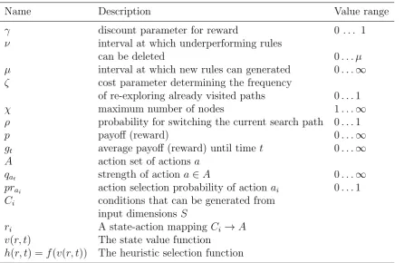
List of Symbols and Abbreviations iv
List of Figures v
List of Tables viii
1 Introduction 1
2 A Computational Framework for Modelling Learning 8
2.1 Introduction . . . 8
2.2 Experience-based Learning . . . 11
2.2.1 Experimental Games Using Simple RL Models . . . . 15
2.2.2 Experimental Games Using Combined Belief and RL models . . . 18
2.2.3 Analytical Approaches with Simple RL Models. . . . 21
2.2.4 Cognitive Approaches . . . 26
2.3 Concept . . . 31
2.4 The Algorithm . . . 34
2.4.1 Reinforcement Learning . . . 35
2.4.2 State Space Partitioning . . . 36
2.4.3 The Complete Algorithm . . . 46
2.4.4 Compact Notation . . . 48
2.5 Relation to Existing Approaches . . . 50
2.6 An Example . . . 52
2.7 Conclusion and Outlook . . . 55
3 Statistical Discrimination 59 3.1 Introduction . . . 59
3.2 Models of Statistical Discrimination . . . 62
3.3 Experiments with Statistical Discrimination . . . 74
3.4 A Reinforcement Learning Model of Statistical Discrimination 77 3.5 Simulations . . . 83
3.5.1 Exploration . . . 84
3.5.1.1 Finding Optimal Learning Parameters . . . 84
3.5.1.2 Variant I . . . 88
3.5.1.3 Variant II . . . 92
3.5.1.4 Variant III . . . 94
3.5.2 Average Results . . . 94
3.5.2.1 Variant I . . . 98
3.5.2.2 Variant II . . . 101
3.5.3 How Persistent is Discrimination? . . . 106
3.5.4 Summary of the Simulation Results . . . 116
3.6 Conclusion . . . 118
4 Network Formation 120 4.1 Introduction . . . 120
4.2 Definitions and Notation . . . 125
4.2.1 Graphs . . . 125
4.2.2 Games on Graphs . . . 127
4.2.3 Stability definitions . . . 128
4.3 Models of Network Formation . . . 129
4.4 Experiments with Network Formation . . . 138
4.5 A Reinforcement Learning Model of Network Formation . . 144
4.6 Simulations . . . 148
4.6.1 Overview . . . 148
4.6.2 Network Properties for Different α . . . 150
4.6.3 Network Structure and Dynamics . . . 153
4.6.4 Memory Effects . . . 158
4.6.5 Summary of the Simulation Results . . . 159
4.7 Applying BRA . . . 162
4.8 Comparison with Empirical Results . . . 166
4.9 Conclusion . . . 171
5 The Market for Primary Care 174 5.1 Introduction . . . 174
5.2 Background . . . 176
5.3 GP Behaviour . . . 178
5.4 Patient Behaviour. . . 189
5.5 Modelling Primary Care . . . 192
5.6 A Reinforcement Learning Model Of Primary Care . . . 194
5.6.1 Overview . . . 195
5.6.3 GP Decisions . . . 198
5.7 Simulations . . . 206
5.7.1 Exploration of the Model . . . 206
5.7.1.1 Parameter Settings and Setup . . . 206
5.7.1.2 Static Analysis . . . 211
5.7.2 Dynamic Analysis . . . 217
5.7.3 Summary of the Simulation Results and Discussion . 220 5.8 Conclusion . . . 225
6 Conclusion 227 Bibliography 233 Appendices 251 A A Scalable ACE Simulation Software Framework 252 A.1 Introduction . . . 252
A.2 Model Representation System . . . 254
A.2.1 The Frame Principle . . . 254
A.2.2 Formal Description as Language . . . 257
A.2.3 Agent Behaviour . . . 263
A.2.4 Agent Communication . . . 269
A.2.5 Other Components . . . 270
A.2.6 Interfaces . . . 270
A.3 Software Architecture. . . 275
A.3.1 Base system . . . 275
A.3.1.1 Architecture and Design . . . 275
A.3.1.2 Implementation . . . 278
A.3.2 Distributed system . . . 278
A.3.2.1 Basic Design Questions . . . 278
A.3.2.2 Architecture and Design . . . 281
A.3.2.3 Implementation . . . 283
A.3.2.4 Examples . . . 288
A.4 Conclusion . . . 290 B Details of the Statistical Discrimination Model 293
C Variance Analysis for the Primary Care Model 296
and Abbreviations
Abbreviation Description Definition
ACE Agent-Based Economics page26
ABM Agent-Based Modelling page28
ACS Anticipation-based Classifier System page28
AI Artificial Intelligence page254
AL Aspiration level page24
API Application Programming Interface page252
BRA Bounded Rationality Algorithm page34
BM Bush-Mosteller model page12
CL Coate/Loury model page62
CBR Case Based Reasoning page24
EWA Experience Weighted Attraction Learning page18
EJB Enterprise Java Beans page285
ER Erev-Roth page15
FFS Fee for service page180
GA Genetic Algorithm page84
GP General Practitioner page176
gsim Generic simulation framework page252
HA Health Authority page194
JEE Java Enterprise Edition page283
JMS Java Messaging System page285
LCS Learning Classifier System page28
PA Payoff assessment model page16
RL Reinforcement learning page2
RMI Remote Method Invocation Protocol page285
2.1 BRA - representation of the state space . . . 39
2.2 BRA - expansion process principle . . . 42
2.3 BRA - generalisation principle . . . 43
2.4 BRA - switching principle . . . 45
2.5 BRA - example 1 . . . 54
2.6 BRA - example 2 . . . 54
3.1 Equilibrium in Coate and Loury’s statistical discrimination model. 67 3.2 Statistical discrimination - model fit model variant I. . . 88
3.3 Statistical discrimination - model fit in model variant II. . . 89
3.4 Statistical discrimination - model fit in model variant III . . . . 89
3.5 Statistical discrimination - hiring rate model variant I . . . 90
3.6 Statistical discrimination - investment rate model variant I . . . 91
3.7 Statistical discrimination - hiring rate model variant II . . . 93
3.8 Statistical discrimination - investment rate model variant II . . 93
3.9 Statistical discrimination - hiring rate model variant III . . . 95
3.10 Statistical discrimination - investment rate model III . . . 95
3.11 Statistical discrimination - average hiring rates for various signal probabilities in model variant I . . . 99
3.12 Statistical discrimination - hiring rates for various signal proba-bilities in model variant I . . . 99
3.13 Statistical discrimination - sample simulation runs for variant I 100 3.14 Statistical discrimination - average hiring rates for various signal probabilities in model variant II . . . 103
3.15 Statistical discrimination - hiring rates for various signal proba-bilities in model variant II . . . 103
3.16 Statistical discrimination - sample simulations for variant II . . 104
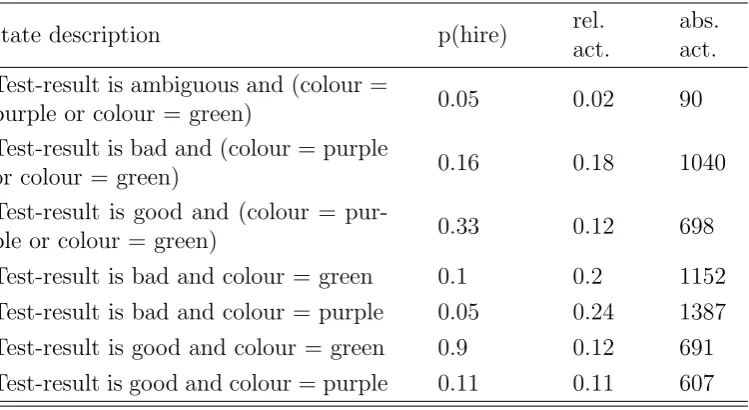
3.17 Statistical discrimination - hiring rates if firms deterministically discriminate (green group) . . . 109
3.18 Statistical discrimination - hiring rates if firms deterministically
discriminate (purple group) . . . 110
3.19 Statistical discrimination - Effect of cost heterogeneity in model variant II . . . 111
3.20 Statistical discrimination - Effect of ex ante beliefs in model variant II . . . 112
3.21 Statistical discrimination - discrimination of green workers for various δf(θ) and ex ante beliefs . . . 116
4.1 Network formation - model fit for various parameters . . . 148
4.2 Network formation - network density for all cost samples . . . . 150
4.3 Network formation - density, stability and fit for the low cost range151 4.4 Network formation - density, stability and fit for the medium cost range . . . 152
4.5 Network formation - density, stability and fit for the high cost range. . . 153
4.6 Network formation - density, stability and fit for the low cost range (BRA model) . . . 164
4.7 Network formation - rule extractions in the low cost range (BRA model) . . . 164
4.8 Network formation - rule extractions in the medium cost range (BRA model) . . . 165
4.9 Network formation - rule extractions in the high cost range (BRA model) . . . 165
4.10 Network formation - average payoff for various α and γ values in the simultaneous linking game. . . 168
4.11 Network formation - density, stability and frequency of Nash networks over time in the simultaneous linking game. . . 169
5.1 Primary care - GP utility function . . . 210
5.2 Primary care - waiting lists (static analysis) . . . 212
5.3 Primary care - referrals (static analysis) . . . 214
5.4 Primary care - GP effort (static analysis) . . . 215
5.5 Primary care - patient utility (static analysis) . . . 216
5.6 Primary care - waiting lists (dynamic analysis). . . 218
5.7 Primary care - referrals (dynamic analysis) . . . 219
5.8 Primary care - GP effort (dynamic analysis) . . . 220
5.9 Primary care - patient utility (dynamic analysis) . . . 221
A.1 Knowledge representation in gsim. . . 255
A.2 The base agent frame in gsim . . . 256
A.3 gsim base architecture . . . 277
2.1 BRA - Summary of notation . . . 46 2.2 BRA - payoffs of the demand game . . . 53 3.1 Statistical discrimination - payoffs of the RL model . . . 78 3.2 Statistical discrimination - description of model variant I . . . . 80 3.3 Statistical discrimination - description of model variant II . . . 81 3.4 Statistical discrimination - description of model variant III . . . 83 3.5 Statistical discrimination - simulation parameters for finding
op-timal RL parameters. . . 87 3.6 Statistical discrimination - simulation parameters for obtaining
average results. . . 97 3.7 Statistical discrimination - rules in model variant I, sample 1 . . 101 3.8 Statistical discrimination - rules in model variant I, sample 2 . . 102 3.9 Statistical discrimination - rules in model variant II, sample 1 . 106 3.10 Statistical discrimination - rules in model variant II, sample 2 . 107 3.11 Statistical Discrimination - rules in model variant II, sample 1 . 114 3.12 Statistical Discrimination - rules in model variant II, sample 1 . 115 4.1 Network formation - RL model parameter settings . . . 146 4.2 Network formation - low cost range network structures . . . 155 4.3 Network formation - medium cost range network structures . . . 156 4.4 Network formation - high cost range network structures . . . 157 4.5 Network formation - network measures for different γ values . . 158 4.6 Network formation - RL model parameter settings for the
simul-taneous linking game . . . 167 4.7 Network formation - Comparison of payoffs of equilibrium
pre-diction, experimental and simulated results in the simultaneous linking game. . . 168 4.8 Network formation - Nash networks visited in the simultaneous
linking game. . . 170
5.1 Primary care - overview of simulation runs . . . 209 5.2 Primary care - utility functions . . . 209 5.3 Primary care - mean and standard deviation of health outcomes
(dynamic analysis) . . . 222 5.4 Primary care - patient loyalty (dynamic analysis) . . . 224 B.1 Statistical Discrimination - average discrimination in model
vari-ant I . . . 294 B.2 Statistical Discrimination - average discrimination in model
Introduction
Economies can be seen as complex dynamics systems: Many autonomous agents interact locally, giving rise to global phenomena such as price levels, growth rates, etc. AsTesfatsion(2006) notes, the study of these macro phe-nomena require strong abstractions and simplifications, which, if removed, quickly make the system intractable. For example, what would happen if the Walrasian Auctioneer would be removed in a standard Walrasian model? Because of this ‘small’ perturbation, the modeller now has to ‘come to grips with challenging issues such as asymmetric information, strategic interaction, expectation formation on the basis of limited information, mu-tual learning, social norms, transaction costs, externalities, market power, predation, collusion, and the possibility of coordination failure (convergence to a Pareto-dominated equilibrium)’ (Tesfatsion 2006). Agent-based com-putational economics (ACE) is a method that has emerged as a novel way to look at the evolution of such equilibria and global phenomena by gen-erating, or ‘growing’ them endogenously (Epstein and Axtell 1996). It is a way to computationally study artificial worlds modelled as dynamic sys-tems of interacting entities. The entities are typically individuals or social
groups such as consumers, firms or players in games. Furthermore, physi-cal entities such as infrastructure or spatial settings might be represented in a computational model. Models are analysed by simulating them in a computer, and interpreting the results that are generated.
A system is called complex if it is composed of interacting units and if has emergent properties, that is, properties arising from the interactions of the agents. FollowingTesfatsion(2006), a system is complex adaptive if the units of the system have some form of pro- and reactive capabilities. There are basically three definitions of complex adaptive systems:
Definition 1. A complex adaptive system is a complex system that in-cludes reactive units, i.e., units capable of exhibiting systematically different
attributes in reaction to changed environmental conditions.
Definition 2. A complex adaptive system is a complex system that includes goal-directed units, i.e., units that are reactive and that direct at least some
of their reactions towards the achievement of built-in (or evolved) goals.
Definition 3. A complex adaptive system is a complex system that includes planner units, i.e., units that are goal-directed and that attempt to exert
some degree of control over their environment to facilitate achievement of
these goals.
experience-based learning, have been widely applied (for details, see chap-ter 3; for an overview see Brenner (2006)). There is no simple rule which models should use which sort of learning; this typically depends on the na-ture of the domain. For example, in environments where habitualisation is a prominent feature, e.g. in repeated game situations, simple reinforce-ment learning matches actual behaviour usually reasonably well. On the other hand, if decisions are less frequent and more important, simple learn-ing mechanisms are not accurate representations. For instance, it could be argued that choosing a doctor (see chapter 4) is a very conscious deci-sion, thus RL would be inappropriate and some mechanism for representing beliefs and judgements would be the more natural choice.
While the role of ACE as a tool for simulating complex systems is straightforward, its role as a paradigm for economic modelling is contro-versial. Typical criticisms of ACE models regard the following points (e.g. Fagiolo et al 2007; Leombruni and Richiardi 2005; Richiardi 2003):
– The lack of standardisation and formalism of ACE models. The sheer mass and heterogeneity of models makes unclear what this approach actually stands for. In general, there are almost no standardised tech-niques to analyse agent-based models, for example, whether and when sensitivity analyses should be conducted, how timing should be inter-preted and so on.
integration of more ‘realism’ in the form of exact agent specifications, there is always a trade-off between descriptive accuracy and analytical tractability. Naturally, the more degrees of freedom a model has, the more difficult it is to map it to available empirical evidence (due to the number of parameters to calibrate).
– The lack of generality and unclear approach to handle results. Whereas it is straightforward to estimate, say, reduced forms, or calculate tran-sition probabilities on empirical data, artificial data can only be cal-ibrated against some empirical benchmark. A result derived from artificial data can only be as good as the underlying simulation is able to replicate the actual real-world process. Furthermore, agent-based models are likely to underidentify actual trends. ACE models are richer, and therefore, create more noise. Another aspect of this problem is ‘equifinality’. Equifinality describes the case when a num-ber of different models may generate similar data, that is, they may equally well explain the same phenomenon but by different processes.
Some ACE modellers view agent-based modelling as a new way of do-ing science (Epstein and Axtell 1996). The main interest of researchers in this area is to discover new rules, theories and test hypotheses about the
processes that generate certain phenomena, and only later derive analytical better models that explain larger classes of phenomena (e.g. Edmonds and Moss 2005). As these modellers typically use their simulations on a mere
auto-referential formalisations that have no link to reality’ (e.g. Fagiolo et al 2007).
The aim of this thesis is to apply RL methods as a means to model adaptive feedback processes. The overall contribution is of a methodological nature. The models presented have the main purpose to demonstrate this method and show how it can be applied to a range of problems. In that sense, the models discussed in the thesis fall into the last category of models: They are mainly of a qualitative nature; empirical validation is not the main interest of the simulations.
The focus of this thesis is reinforcement learning. Reinforcement learn-ing is a very simple experience based learnlearn-ing approach; agents learn by trial and error. It has often been used in the ACE literature, but often ad-hoc or in simple models. Moreover, there are only few approaches which integrate experience-based learning with cognitive elements such as beliefs.
The objectives of the thesis are to
1. Develop a new computational approach that integrates RL with sim-ple cognitive elements. It shall provide a new approach of modelling human decision processes.
2. Apply RL to economic, mainly game-theory models and contribute to the learning literature in this field. As the use of simulations allows to build more complex models, an important aspect of this thesis is to build a ’bridge’ between pure game theory and empirical results of ex-perimental game theory. A recurring topic is therefore the comparison with experimental evidence.
domains. Here, the question is how RL can be used to enrich the analysis of more applied, real-world models.
As the methodological basis, chapter2reviews RL in the economic liter-ature and develops a general learning framework, combining reinforcement and rule learning. The motivation is to provide an alternative, generic way of representing agent decision mechanisms in a unified framework for several classes of models. It tries to go beyond simplistic fomalisations of adaptive capabilities such as simple RL, but to keep computational complexity within bounds. Chapter 3 applies this approach to a model of statistical discrimi-nation. It is shown that the framework is capable of reproducing patterns of actual human behaviour in game-theoretic experiments. Chapter 4is an application of RL to network formation. Results of the learning process are compared with axiomatic results for perfectly rational players. A modified version of the model is then used to reproduce an experiment and to com-pare its behaviour with observed human behaviour. A very different model is presented in chapter5. While the purpose of the first chapters is to apply and analyse learning in rather simple settings, the purpose of this chapter is to use it in a complex setting with many influencing variables. The re-quirements for adaptation in this application are very different from that discussed before: In the model, doctors decide about treatment patterns, quality and their own workload. Patients choose doctors based on their own experience and recommendations of other consumers. Several simulations using different learning and choice scenarios are compared.
The models have been implemented in their own software framework, providing the learning features used in the thesis. Appendix A describes the architecture and implementation of the software.
– It adds a novel algorithm for representing learning in artificial agents. This approach has been published in Schuster (2012).
– It applies RL to statistical discrimination games. It belongs thus to the few dynamic models in this area, and is to the knowledge of the author the first using an RL approach.
– It applies RL to strategic network formation games. So far, adaptation in the strategic network formation literature has received almost no attention. Here, adaptation is applied for the first time to the well-known connections model of Jackson and Wolinsky (1996).
A Computational Framework
for Modelling Learning
2.1
Introduction
The perfectly informed and rational homo oeconomicus has often been crit-icised as too unrealistic - humans would not have the computational power to calculate the best decisions, taking into account all information and all possible outcomes. Already Simon (Simon 1956b) argued to use simpler, psychologically more plausible algorithms. While the argument of bounded rationality is frequently used as critique of the standard economic model, the argument remains, however, vague (Simon 2000) - meaning usually every-thing that is not classical economics, ranging, for example, from systematic errors people make in judgements to the research on decision heuristics as an alternative form of decision making.
Common to all critiques of perfect rationality is that humans are not capable of doing the computations required by a homo oeconomicus, but are bound to commit errors and misjudgements. As some psychologists (e.g.
Gigerenzer and Goldstein 1996; Lopes 1994) point out, most alternative
models are still based on the fundamental assumption that expected utility and Bayesian reasoning are the basis for all human decision making under uncertainty. For example, subjective expected utility theory acknowledged that individuals are not fully informed, and replaced objective probabilities with subjective; however, the basis for reasoning remained the same.
In the sociological and psychological literature, a vast amount of evi-dence has been collected to show experimentally how this classical model can fail. Formalisation, however, is rare. An example is Prospect Theory (Kahnemann and Tversky 1979). The main argument of Prospect Theory is that people value future losses more highly than potential gains. Prospect theory proposes an S-shaped value function that is concave for gains, and convex for losses. That is, individuals become risk avoiding the higher the potential losses, and risk seeking the greater the potential gains. Another aspect of the value function has been characterised by loss aversion, which is usually represented by a steeper slope of the curve in the loss area. These aspects have been used to explain apparently irrational, as well as loss avoid-ing behaviour in many psychological experiments. Psychologists have also emphasised that humans process information not as the Bayesian paradigm postulates, but rather crudely by using decision heuristics and cues from their environment. In the field of cognitive psychology bounded rational-ity became almost exclusively associated with this perspective in cognitive psychology. The behavioural aspect of bounded rationality (like learning by doing) has been neglected or not seen as a subject for this discipline (Gigerenzer and Goldstein 1996).
With RL approaches a more behavioural dimension has become available in (behavioural) game theory. In pure stimulus-response models, agents learn by trial and error without any explicit knowledge representation (e.g Roth and Erev 1995). Some authors combine experience learning with foresight
in mixed models as in fictitious play (Camerer and Ho 1999). Some ACE models are based on similar concepts (see Brenner (2006) for an overview); especially classifier systems have received interest to represent a simple form of rule learning (e.g. Kirman and Vriend 2001a;LeBaron et al 1999).
Another angle of decision making can be seen in cognitive architectures. Architectures such as ACT-R (e.g. Anderson 1993) and Soar (e.g. Lehman et al 2003) try to simulate human decision-making as a computer program.
Most of them focus on the working of the mind when solving, say, math-ematical problems and model in detail what processing steps are involved in solving such problems. More recently, Sun showed how his cognitive ar-chitecture CLARION (Sun and Slusarz 2005) can be connected with social simulation. In this approach, the environment of an organism can, in con-trast to the classical architectures, be represented in an agent’s mind (Sun and Naveh 2007).
In this chapter, a computational model of bounded rationality is devel-oped that addresses the tension between simplifying representations as pure stimulus-response learning on the one end of the spectrum, and often com-plex higher levels of cognition on the other end. It is most closely related to mixed models and classifier systems, and has analogies with Sun’s applica-tion of CLARION. However, there is no distinct social or economic approach to individual learning. The algorithm described in this paper attempts to fill this gap.
some detail. Then, a simple conceptual framework based on Simon’s con-cept of bounded rationality (Simon 1956b) is described, before outlining concept and algorithm in more detail. The algorithm is then related to the existing approaches in the literature. A simple simulation illustrates how the algorithm works. The conclusion also outlines how the framework is related to the learning problems in the applications in chapters 3to 5.
2.2
Experience-based Learning
other strategies. If the other strategies fare better, the player can then switch his behaviour. While experience is necessary to learn in fictitious play, it requires also a cognitive component, namely the reflection upon other players’ actions. Pure belief-based approaches do not use the feed-back coming from own activities. A typical example is Bayesian learning, which updates beliefs about future states an agent will be in. Cognitive architectures from Psychology can be seen as a similar example. These approaches aim to model mental processes in the brain, and as such are typically independent of concrete experience.
The aim of this chapter is to develop an algorithm that can be ap-plied to a wide range of ACE modelling problems. Thus, approaches that do not require prior knowledge about the domain are the most relevant. Experience-based learning methods are a natural candidate for this, since they acquire knowledge incrementally and base decisions on that knowl-edge. The literature reviewed here looks therefore mainly at experience learning, in particular reinforcement learning, but not pure belief-based learning. Furthermore, throughout the thesis, RL will be used as a syn-onym for any experience-based learning method that is based on RL.
In RL, agents learn to choose actions that were successful in the past more often, while they avoid actions that led to unsatisfactory outcomes. This is referred to as the ‘Law of effect’. A basic learning model was first formalised by Bush and Mosteller (BM) (Bush and Mosteller 1955). Ac-cording to BM, the choice probabilities p of an action at a given time can be computed according to
is a mathematical operator that describes the new quantity of p after the reward is applied. It is a short form to describe the stepwise update of reinforcements. Most learning models generalise the BM idea to a time-discounted version. The main components typically are:
– An action set A from which an action a is chosen, and payoffs π
associated with them;
– An action strength function that updates the experience over time. The typical function is introduced in Roth and Erev (1995):
qk(t+ 1) =qk(t) +π(t) (2.2)
which updates the strengthqof thek-th action with the current payoff (Roth and Erev 1995).
– A selection function that selects successful actions based on the qk. This selection function is usually based on Luce’s choice theorem (Luce 1959):
pk =
qk
∑
qj
(2.3) This function computes the choice probability of action k relative to its strength qk.
– Cumulative RL without aspirations (Roth and Erev 1995; Erev and Roth 1998; Laslier et al 2001; Laslier and Walliser 2005; Beggs 2005;
Rustichini 1999; Camerer and Ho 1999), which are all based on the
original BM model described above. Many analytical approaches use the simple version in combination with simple decision problems where adjustment to changing environments does not play a role; the problem does not exist in this case. Other models, mainly of are more empirical nature, vary the base model by adding forgetting and experimentation parameters (Erev and Roth 1998) or simple beliefs (Camerer and Ho 1999) to counterbalance the effect of excessive cu-mulation.
– Averaging mechanisms (Karandikar et al 1998; Mookherjee and So-pher 1994;1997;Sarin and Vahid 2001;Gilboa and Schmeidler 1996).
In principle, average reinforcements can be interpreted as a form of be-lief learning, namely as an expected future reward. The advantage is that agents can adjust reasonably fast to changes in the environment.
– Aspiration level models with cumulative RL (e.g Boergers and Sarin 2000) or averaging mechanisms (e.g. Karandikar et al 1998; Bendor
et al 2001b; Napel 2003; Gotts et al 2007); see also Bendor et al
proportional to their expected payoffs, thereby achieving a similar ex-ploration effect once their environment changes and payoffs decrease. The advantage of this approach is that lock-in into optimal choices is supported, at the same time not being deterministic if payoffs fall below the aspiration level.
2.2.1
Experimental Games Using Simple RL Models
One main motivation of many models has been the search for learning rules that predict experimental data better than the standard equilibrium predic-tion under full informapredic-tion (e.g. Roth and Erev 1995; Erev and Roth 1998; Mookherjee and Sopher 1994;1997;Chen and Tang 1998).
In their seminal work, Erev and Roth (Roth and Erev 1995) consider three variants of the base model (equations (2.2) and (2.3)); later referred to as ER models). The first uses cutoff parameters for high and low selection probabilities: Actions above the upper cutoff are played with probability 1, below the lower with probability 0. In the second model, a parameter ϵ
sets the probability with which a random action is chosen. This allows for persistent experimentation. The third variant includes a recency parameter
actual behaviour did not converge to equilibrium. Moreover, experimental data showed differences in medium- and long-term outcomes. The RL model could replicate such switches.
Later, in Erev and Roth (1998), they apply simple RL to a wider col-lection of experimental data based on mixed-strategy games; this makes convergence more difficult, since no player has an incentive to stick to a pure strategy. Additional to the simple model, they allow for alternatives with more sophisticated learning. Three models are compared: Model (1) is simple RL as in equations (2.2) and (2.3). Model (2) combines forgetting and generalisation, i.e. qk(t+ 1) = (1−ϕ)qk(t) +Ek(j, π(t)), whereE is a function determining how playing strategy k affects similar strategies j. In the considered 2-player games, they set Ek(j, π(t)) =π(1−ϵ) if j =k and
Ek(j, π(t)) = π(t)ϵ/(M −1) (where M is the number of pure strategies) otherwise. That is, depending on ϵ, players generalise rewards in a way that leads to experimentation among similar strategies. In model (3) some simple beliefs are integrated in the form of limited (only own payoffs are known) and full information (also opponents’ payoffs are known) fictitious play. In the first case, the update function is augmented by an expected payoff parameter, in the latter the action probability is determined consid-ering the value of alternative strategies. After fitting the data, they find that adding more knowledge in the form of beliefs and expectations does not add to the predictive power of RL. Usually, the simplest models pre-dict behaviour accurately. Adding adaptation parameters like recency and experimentation improves the fit of simple RL, but fictitious play does not.
and Roth (1998), they find that this model predicts the data at least as well as simple RL.
Mookherjee and Sopher (Mookherjee and Sopher 1994;1997) conducted experiments with constant sum games. In their early experiment only two choices were available. Players learnt to play their minimax strategies. In Mookherjee and Sopher (1997) they find that experimental results devi-ate considerably from equilibrium predictions in games with at least four strategies. Instead of cumulative payoffs, here qk is some average measure of action k. Furthermore, they use the exponential selection function
pk(t+ 1) = e λqk
∑
eλqj (2.4)
(where λ is a choice parameter). After comparing also belief-based learn-ing rules, they further conclude that the RL predictions match the reality closest. Using different averaging mechanisms, their data suggest that play-ers’ memory is rather short, and that they form expectations about future payoffs.
Chen and Tang (1998) use a cumulative reinforcement function as in equation 2.2 with an exponential selection rule as in equation 2.4. Ap-plying it to public good provision games, they compare its performance in predicting experimental data with fictitious play as well as the equilibrium prediction. They find that the empirical results deviate from the equilib-rium prediction, which predicts the data worst. The RL mechanism fits data better than fictitious play.
defined as
et =
1, x is played at t 0, x is not played at t,
. The cumulative update function in equation 2.2 can be written as
qk(t+ 1) =qk(t) +π(t)et (2.5)
.
Then, let the cumulative payoff until time t be vt = ∑s<tπs. Let ∆p(t) = p(t + 1)− p(t) denote the incremental change in the probabil-ity vector e at time t. Because of equations 2.5 and 2.3 one can write ∆p(t) = (πt/vt)(et−p(t)), that is the incremental impact of new experience diminishes over time at a rate of the order of 1/t. Arthur proposed a model of the form ∆p(t) = [π(t)/(Ctν+π(t))][e
tp(t)]. In that model, the incremen-tal impact of the current payoffs on the action probabilities decreases over time at a rate of the power of t, which is estimated from data. This is an-other way of solving the problem of just accumulating experience over time without possibilities to revise choices. Arthur fits the model to single person multi-armed bandit experimental data and finds no systematic differences between simulated and human learning (from Young (1993),pp.11-13).
2.2.2
Experimental Games Using Combined Belief and
RL models
N(t) =ρ∗N(t−1) + 1 (2.6) and
Aji(t) = ϕN(t−1)A j
i(t−1) + [δ+ (1−δ)I(s j
i, si(t))]π(s j
i, si(t))
N(t) (2.7)
N(t) denotes the experience weight, andAji(t) the attraction of strategy
j for individual i. si(t) is i’s strategy at time t, and si are the strategies of all other players. The function I(sji, si(t)) is an indicator function and equals 1 if sji = si(t), and 0 otherwise. The payoff π is obtained by player
i if he chooses sji, given the behaviour of the other players si(t). ρ, ϕ, and
δ are the parameters of the model. The initial values of N(t) andAji(t) are priors and may be initialised with some experience level the players already have.
For N(0) = 1 and ρ = δ = 0, the model reduces to pure cumulative reinforcement learning. For δ > 0, experience collection is expanded to actions not played by observing the other players in the game. If ρ=ϕ and
δ = 1, the model reduces to weighted fictitious play; for other parameters, the learning represents a mix of RL and fictitious play.
The action selection function has an exponential form and is given by
Pij(t+ 1) = e λAji(t)
∑mi
k=1eλA
k i(t)
(2.8)
Camerer and Ho test this model with data from constant-sum games, among them the games from Mookherjee and Sopher (1997), and com-pare EWA with random, simple RL and belief-based outcomes. The results show that belief-based learning predicts better than EWA in the simpler 4-strategies games, but worse in more complex 6-strategy games. Contrary to Mookherjee and Sopher(1997), they find that belief-based learning con-verges better than RL learning, which they attribute to differences in the model. For example, Mookherjee and Sopher allowed similar strategies to influence each other, and they used average instead of cumulative reinforce-ments; both factors favour their RL rule, while in EWA, these aspects are reflected in the belief component.
EWA has been criticised as being too complex and requiring overly many parameters. Therefore, Camerer and Ho developed in Camerer et al(2007) a simplified version of EWA, ‘self-tuning EWA’, by fixing most of the pa-rameters and only estimating ϕ and δ with dynamic functions. If a player detects a change in opponents’ play, ϕ is adjusted to allowing more experi-mentation, and vice versa (becoming pure RL in stationary environments). The attention function sets δ to 1 if the foregone payoffs are higher than the actual received payoff, so that alternative strategies are reinforced, and the agent eventually may switch to one of the superior actions. If there is no better choice available, δ is set to 0, thereby supporting an RL-like lock-in into the best response strategy. Comparing the predictive power of full and simple EWA, they find that self-tuning EWA is not as good as the original approach, but produces very similar results. This applies especially if parameters are estimated for the same class of games. Self-tuning EWA predicts better if parameters are estimated jointly for different games.
games with two players. They find that PA fits best to the data, followed by EWA and RL. When estimating parameters over different games (pooling) PA does best. An exception is cost-sharing games with an average-cost distribution among players. Under this mechanism, the cost is distributed evenly, and thus experimentation in one agent triggers experimentation in the other players. None of the models converged to the observed data.
Stahl (2000) develops a model in which players learn to choose among different strategies following simple decision rules. Players know the strate-gies played by their opponents. Analogously to other learning models, rules in the rule space that were successful in the past are more likely to be se-lected. The rule space can be thought of as composed of basic, or ‘archetyp-ical’, rules, from which more complex behaviour can be constructed. The evidence of every rule is assessed, and the probability of choosing that rule is derived using an exponential selection rule. This evidence is, e.g., the ex-pected payoff given the opponent’s strategy in t-1. Based on such reasoning, Stahl defines five strategies (e.g. strictly dominated vs. Nash equilibrium strategies) which are first tested in experiments, and then fitted to the data. He finds that the model fits the data better than the equilibrium prediction and random outcomes. The model uses nine parameters, which is found to be the required minimum to fit the data well. Furthermore, evidence from the experiments suggests that real humans do not gather evidence about all rules as proposed by the model, but rather focus on subsets.
2.2.3
Analytical Approaches with Simple RL Models
the-ory. Early work mostly established results for limited classes of games or simple one-player decisions. Only more recent articles (e.g. Beggs 2005; Hopkins and Posch 2005;Gotts et al 2007) could state more general results
for the boundary behaviour for the process, and larger classes of games.
ER models Some authors have analysed the ER learning rule (Rustichini 1999; Laslier and Walliser 2005; Beggs 2005; Rustichini 1999;Hopkins and
Posch 2005) in single decision and game contexts.
Rustichini (1999) considers optimal properties of selection rules under full and partial information in a single player context. Under full infor-mation the player knows opponents’ strategies, under partial inforinfor-mation only its own actions. He finds that with a linear rule (as in equation (2.3)), convergence to the optimal choice is guaranteed. It is not with the exponen-tial rule, which weights differences between payoffs higher and thus might speed learning up. Moreover, exponential procedures (as in equation (2.4)) are best in the full information case, but not for partial information: Linear learning is too slow in full information environments, so the process is more likely to lock into sub-optimal interior points of the strategy space, rather than the optimum.
that the process converges with probability 1.
Building on stochastic approximation theory,Beggs(2005) considers 2x2 constant-sum games with unique pure or mixed equilibria and generalises Laslier et al (2001). Players using RL cannot be forced permanently below their minimax payoff, independent of their opponent’s strategy. Similarly, dominated strategies are always eliminated over the course of time. If both players play RL, the probability that both players converge to the unique equilibrium, tends towards 1.
Hopkins and Posch (2005) provide more general results about the re-lationship of the RL processes with the well-analysed replicator dynamics approach from evolutionary game theory (Smith 1982). They find that Arthur’s model (Arthur 1993) as well as ER-type models converge only to boundary points which are a Nash equilibrium. This is easier to show for the Arthur model because the action strength updates (step sizes) are of the same size, while the reinforcements in ER can change at different rates. They show that RL will not converge to boundary points that are linearly unstable under the replicator dynamics.
Aspiration level models The reinforcement problem in aspiration level models has been also been studied by several authors, and has been sur-veyed in-depth by Bendor et al (2001a). Here, some representatives of this approach are described.
Gilboa and Schmeidler(1996) present a case-based reasoning (CBR) ap-proach. The decision maker faces a number of different situations or ‘states’, and must make a choice in such situations. In dynamic environments, aspi-ration level (AL) updating rules have to be ambitious enough to search for the best result in various situations. In more static environments, it must be realistic, i.e. close to actual payoffs. Both properties must be combined, as a way to search ambitiously for a best strategy, and then to stick to this choice after the expected values of the strategies can be estimated. They show that under these conditions, a case-based decision-maker can learn to become an expected-utility maximiser.
Extending their work on RL with fixed AL, Boergers and Sarin (1997) develop a model with endogenous aspirations and cumulative rewards. In Boergers and Sarin (2000), a single player chooses between two strategies. They show that the process can converge to the optimal choice. Endogenous aspiration levels improve performance by avoiding high dissatisfaction with even the best available strategies, but can lead to probability matching. During probability matching, both strategies are played at the same proba-bility at which they generate benefits, whereas optimal strategies should be played with probabilities close to 1 for behaviour to be considered ‘rational’. This can happen when the initial aspiration levels are too high, so that also dynamic adaptation of the aspiration level cannot lead to a lock-in.
games. Karandikar et al (1998) first analysed a prisoner’s dilemma. The aspiration levels of both players are updated simultaneously with the re-ceived reward, and approximate long-run averages. The main result is that cooperation is sustained if there are no trembles (i.e., externally imposed changes or noise on the AL’s) to the AL’s and the speed of updating the AL’s is low. Introducing perturbations into the AL changes the process, and may lead to different equilibria. However, in the long run, the process returns to the cooperation path. The intuition behind these results is that the mutual dissatisfaction with non-cooperative payoffs triggers experimen-tation until some state is achieved that yields high enough satisfaction (the point where AL and current payoff converge).
Karandikar et al (1998) is modified and extended to arbitrary games and a larger class of learning rules in Bendor et al(2001b). Similarly,Napel (2003) applies the model to an ultimatum game and shows that in the long run players almost surely achieve the equilibrium state. Which equilibrium depends on the initial conditions and the stability of aspirations, which are allowed to vary randomly. If such trembles are rare and learning is slow, the available surplus will be shared efficiently. If there are perturbations in the aspiration level, any equilibrium is supported.
2.2.4
Cognitive Approaches
This section reviews two approaches of a more cognitive nature stemming from Artifical Intelligence AI. Still being based on own experience, they provide mechanisms to make the agent aware of different conditions in the environment.
CLARION The cognitive architecture CLARION (e.g. Sun and Slusarz 2005) was designed to capture implicit and explicit learning processes in
humans. The main assumption is that there are two different levels of learning: A subsymbolic ‘bottom’ level and a symbolic ‘top’ level. The ‘bottom’ level represents low-skill, often repetitive tasks for which learning proceeds in a trial-and-error fashion. Knowledge on this level is typically not accessible, and it is difficult to express such skills with language. On the symbolic level, knowledge is directly accessible and can be expressed with language. This level typically represents more complex knowledge. It can be acquired by experience, but also by explicit teaching.
The input state is made up of a number of dimensions, and each di-mension may specify a number of possible value or value ranges. Action selection takes place using RL in the bottom level, or by firing production rules on the top level. Which level is used is determined stochastically. Af-ter the action was performed, top and bottom levels are updated with the feedback received from the environment.
At the top level, the rule conditions are constructed out of the input dimensions, their consequents from actions available to the agent. The rules are, for compliance with the bottom level, implemented as network. Rule extraction, specialisation and generalisation are determined by feedback from the subsymbolic level: If there is no rule matching the current state and the action performed well according to some performance criterion, a new rule is created with the current state as the condition, and the performed bottom level action as consequent. If rules matching the current condition exist and the action was successful, the matching rules are replaced by a generalised version by adding another input element to the condition. The covered rules are deactivated, but might become reactivated if specialisation is applied to the new rule at a later stage. Conversely, specialisation means the removal of an input value from the condition and is triggered when the result of an action was not successful in the specified condition. Deactivated rules are reactivated if the specialised rule does not cover them any more. An information gain measure that estimates the performance of rules under different conditions serves as the success criterion.
Learning Classifier Systems Learning Classifier Systems (LCS) also aim at the extraction of rules. The basic idea is to start with a set of initial rules (classifiers) and to evolve this set over time by application of mechanisms for modification, deletion and addition of new rules. Whereas earlier LCS, as introduced by Holland (1975), relied mostly on the Genetic Algorithms paradigm, newer versions have more in common with RL ap-proaches and so have also been described as generalised RL (Sigaud and Wilson 2007).
An LCS consists of a population of classifiers. A classifier contains a condition part, an action part, and an estimation of the expected reward. Typically, the condition part consists of the three basic tests 0 (property does not exist), 1 (property exists) and #. # represents a generalisation and stands for both 0 or 1. A classifier has one action as a consequent, but typically several classifiers match a condition in the environment and hence compete with each other. The action to be executed is then selected according to some RL mechanism (e.g., the ϵ-greedy policy, which selects the best-performing action at a rate of ϵ, 0 < ϵ <1 tries a random action).
Many LCS use a Genetic Algorithm to create new rules by selecting and recombining the fittest classifiers from the population (where fitness is, e.g., the expected reward received from the environment). A covering operator is called whenever the set of matching classifiers is empty. The operator adds a classifier matching the current situation with a randomly chosen action to the population. Sophisticated systems may limit the population size, and add corresponding eviction and generalisation procedures.
build a model of transitions. A specialisation mechanism is applied when the classifier oscillates between correct and incorrect predictions, indicating that a splitting of the condition might improve the match. Generalisation is based on complex algorithms that estimate whether generalisation will re-sult in an improvement (see also Sigaud and Wilson (2007) for an overview of LCS).
Applications in Economics have usually used Holland-type classifiers. Markets of different kinds have been modelled using LCS, for example, the market for electricity (Bagnall and Smith 2005), for fish (Kirman and Vriend 2001b), or stock markets (e.g. LeBaron et al 1999).
In Bagnall and Smith (2005), the UK electricity market is modelled. In the model, there are a number of electricity generating agents. Each agent must produce an offer bid per day for the amount of electricity it wants to produce. The strategies are determined by three factors - capacity constraints, demand and capacity premiums (for particular time slots in a trading period). By this, a 10-bit vector of states, denoting different demand, constraint and premium situations is constructed. The model is used to model various scenarios. For example, they reproduce actual, observed bidding behaviour.
out that loyalty develops as buyers and sellers realise simultaneously the benefits: Returning customers allow better planning of a seller’s stock and continuous profit flow, for which lower prices are accepted; because of these, customers learn to return.
The stock market model ofLeBaron et al(1999) aims to reproduce actual stock market behaviour in an artificial stock market. In the market, there are trader agents whose task is to make forecasts about the future price of assets. The expected price is used in their demand functions, which then determines the amount of assets to purchase. The agents base their forecasts on hypotheses or candidate rules, of which a single agent maintains 100. These rules map conditions of the environment into forecasts. The state vector is 12 bits long. The conditions are given by dividend/price ratios and comparisons between current price and average prices, which describe the value of an asset given the market conditions. LeBaron et al(1999) are able to reproduce features of price time series taken from real markets.
2.3
Concept
As the literature overview in the previous section showed, there is substan-tial literature, mainly in the area of simple games. Fewer authors attempted to develop cognitive strategic models. Each approach has its limitations with respect so ACE modelling. Thus, a cognitive architecture covers psy-chological details social scientists are often not interested in. LCS are a rather technical approach to learning. For some domains and problems, the representation system might not be adequate (Schuurmans and Schaeffer 1989). In particular, the representation of knowledge as bit strings may
introduce problems. For example, it is difficult to represent more abstract knowledge like relational operators such as greater, smaller etc. To cover large value spaces, it would be necessary to represent each single value as bit in the string. Thus, representing fish prices from 0 to 1000 in Kir-man and Vriend (2001b) would become difficult, or at least require implicit knowledge about the domain to set up the classifiers adequately.
The main contribution of the computational approach presented here is the formulation of a learning model that covers simple as well as more cognitive modes of learning. From a theoretical point of view, it should be a mixed model. As a computer model, it should be valid in the sense of reflecting simple, but realistic decision making, and simple in the sense that it focuses only on decision mechanisms in social and economic contexts. It should therefore be more specific as a cognitive architecture, and have more natural and broader representation features as LCS.
– The set of behaviour alternatives A
– The set of choice alternatives A′ for bounded rational or
computa-tionally less powerful individuals; this set may be only a subset of
A.
– Possible future states S
– Payoffs connected withS, represented as a function of S, V(s).
– Probabilities for S. There is uncertainty which state occurs after a particular behaviour, i.e. there may be more than one.
Bounded rational individuals do not typically know the mapping from be-haviour alternatives A to future welfare V(s). A possible strategy to learn about the occurrence and the desirability of these future states is accord-ing to Simon: Start with a mappaccord-ing of each action alternative a ∈ A to the whole set of S. Using a utility function such as V(s) ∈ {−1,0,+1}, find S′ ⊂ S such that (expected) V(s) = 1. Then gather information to refine the mapping A → S′ (i.e., which actions lead to which result under
certain conditions) and search for feasible actions A′ ∈ A that map to S′
(Simon 1956b). In other words, an agent’s goal is to find the states which satisfy its needs, by exploring the state-action space by applying alternative behaviours.
able to evaluate the results of actions or the consequences of a change of state (Markham 1999). It is assumed that an agent is only interested in its own welfare, and its goal is to find suitable behaviour strategies that optimise utility under different conditions. Information processing and memory are costly, so that the internal model being built has to be minimal and efficient with respect to the agent’s welfare. The main principles an algorithm has to account for can roughly be summarised as follows:
Evaluating cognitive cues In any state of the environment, the agent must be able to choose an action. If low or even negative rewards are experienced, the agent can attempt to apply a different action. If this fails to improve the agent’s welfare, this is a hint to pay attention to more cues from the environment and distinguish better between situations.
Updating a cognitive model If the environment changes, some aspects of the internal model might become obsolete. The agent will then experience a change in utility. In certain states, learning a new behaviour might be sufficient. However, it might also be that the representation of the state is not accurate anymore (e.g. a new type of agent appears). In this case, the representation has to be changed, e.g. by removing old representations and start the search process anew for certain parts of the model.
A similar idea has been used in Gifford (2005). In this model, agents have limited information about future outcomes of opportunities (e.g. stock returns), and have to decide whether to evaluate new, or to stick to old behaviours (e.g. buying a new stock). Attention is a scarce resource, so that evaluating alternatives becomes costly. It turns out that the higher this cost is, the more ‘irrational’ the behaviour; if cost is neglected, and agents can spend more effort on evaluating future expected states, behaviour approximates more rational decision-making.
2.4
The Algorithm
The basic idea of the ‘Bounded Rationality Algorithm’ (BRA) is to build an internal, flexible model of the environment the agent lives in. The en-vironment is accessible by the input state s defining the current ‘situation’ the agent is in. The input state is matched with an internal symbolic rep-resentation Ci ∈ C ={C1. . . Cn} of the state. The agent then chooses an action according to the general form ri : Ci → A. A is the action set, C is the set of all possible conditions that can be generated from the input dimensions, and Ci is a collection of conditions derived from C.
2.4.1
Reinforcement Learning
RL is used to implement the dynamic aspect of knowledge generation in the model. In each state agents learn by trial and error which action to apply in a given state. Successful actions are rewarded. Actions which yield a higher reward are selected with a high probability in the future, whereas bad actions, receiving a lower reward, are selected less often. The history of these reinforcements is summarised as action strength q. Whenever an action a has been applied, the strength is updated with the reward p(t) observed for that action by the following equation (Sutton and Barto 1998):
q(at) =q(at−1) +γ(p(t)−q(at−1)) (2.9)
This action-value function updates the strength of the current action based on the weight γ of previous experiences and the current reward. It is a method to approximate the true value of q(a) out of a sample of values. The smaller γ, the stronger the impact of past experiences; conversely, for
γ = 1 only the reward of the last action is considered, and all previous experiences discarded. Thus γ determines the speed of updates.
In the next step, the action probability is calculated according to the selection function:
pr(ai,t+1) =
eq(ai)/α
∑
jeq(aj)/α
(2.10) This exponential selection function determines each action’s selection prob-ability depending on its own strength relative to the strengths of the alter-native actions. The parameter αis a parameter that determines the rate of exploration. The influence of the action strength on the selection probabil-ity decreases as α grows. For large α, the selection probabilities approach uniform values. Sutton and Barto (1998) report that for many problems,
approaching 1 translate into selection probabilities smaller than the original action strengths, so that too large values quickly stop being useful for the learner. Finally, as α → ∞, each choice becomes equally likely.
2.4.2
State Space Partitioning
Learning by doing as described above happens for a given state s. This section describes how states are represented and perceived in the agent’s internal world model.
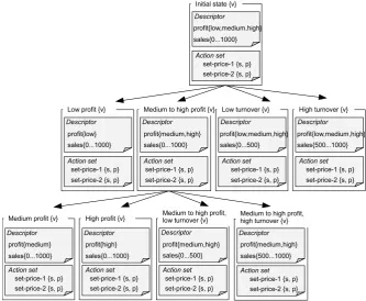
Representation The state s is represented internally as a collection of attributes {att1. . . atti}. Each attribute can have a number of possible values, for example nominal values such as ‘low’ or ‘high’, or numerical ranges, e.g. 0-1000. Attributes are connected by simple predicate logic. For example the predicate ‘(profit=low or profit=medium or profit=high)
and (sales 0 < sales < 1000)’ could describe the situation of a firm in the dimensions profit and sales. This representation is called a ‘state descriptor’, and formally denoted Ci. To each state descriptor actions are bound from which the action policy for this state can be learnt. In the firm example, actions could be an array of price levels. This binding constitutes formally the mapping ri :Ci →A.
descrip-tions are ‘expanded’ from the predicates at higher levels. Coarser grained descriptors can be generalised again if the more detailed descriptors do not perform better than the parent. Which descriptions are expanded depends on a heuristic evaluation function, which here is the agent’s utility. Each state descriptor has a value that describes this utility. The task of the search process is thus to find the level of detail that describes the environment in such a way that generates the highest welfare for the agent.
Depth-first search principle The path the expansion mechanism takes follows a depth-first search paradigm. If finer grained descriptions increase welfare this path is followed further, that is, the mechanism assumes that the most accurate state descriptions are best. Using a tree-search approach, this corresponds to a process in which a single node on level h is expanded to level h+ 1 according to some performance criterion, while the siblings on level h are not taken into account. The path this process takes is rep-resented by the ‘search path’. Each node the process expands is added to this path, and removed when it is generalised. The search path is thus a list which contains all nodes of the tree that are relevant for the model specialisation and generalisation methods. These methods are described in the next paragraphs.
discrete values, one value is picked randomly. Attribute values representing numeric ranges are split in half. For each partitioned attribute a new con-dition is created containing the partitioned attribute values or value range, and the remaining original attribute values (i.e. the number of successor nodes equals the number of attributes × 2 in the original condition). The conjunction of the predicates of the resulting level (after reduction) is equiv-alent to the expression of the parent node. By mapping A to each newly created condition set the new descriptors R′ are generated. The path from
each r′ ∈R′ up to the root node is set as search path (without duplicates).
The conjunction of state descriptions with no children in the tree is then equivalent to the initial state description. The RL mechanism selects ac-tions only from the matching leaf descriptors. There might be, depending on the paths that have been expanded, overlapping descriptors. In this case, for deciding which state is activated some conflict resolution has to be applied. This could be the selection of random node, or the node with the highest value. In the implementation used for the models of the thesis (see also appendix A.2.3), a random node is selected.
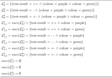
For example, going back to the firm example above, of the initial, exhaus-tive descriptionC′
initial= (profit=loworprofit=mediumorprofit=high)and (0<sales<1000) the attribute profit is selected, and of its value range the value ‘high’. The value space of the attribute is divided into the expression ‘profit=low or profit=medium’ and ‘profit=high’, respectively. The result-ing specialised state descriptions are C′
Figure 2.1: The agent’s representation of the state space after partitioning all possible profit situations. Each state is described by a set of attributes and an action set. Actions executed in this state are updated with strengths s and selected with probabilitiesp, which are determined by rewards. The rewards also determine the state valuev.
Model specialisation and generalisation With the state expansion mechanism it is possible to specialise the conditions in the state-action space in many ways. A heuristic evaluation function determines the direction of this process. This function is calculated as follows: First, the value of a state at time t is calculated as
v(r, t) =v(r, t−1) +λ(q(at)−v(r, t−1)) (2.11)
where q(at) is the reward of the executed action in the state described by
speed of update is governed by the parameter λ ∗.
Before an expansion happens, some constraints have to be satisfied: The parameter χ limits the maximum number of nodes the tree can have, i.e. the maximum number of situations the agent can differentiate. New states can only be evolved at the cost of ‘forgetting’ other state descriptions (see below for deletion). Furthermore, since the deletion of nodes might occur, it is possible that state descriptions that were deleted are expanded again, so that endless cycles of generalisation and specialisation occur. The right balance has to be found depending on the stability of the environment; preventing many visits of identical descriptions too early can be harmful if the environment changes; on the other hand, the agent should be allowed not to become trapped into useless expansion/retraction cycles. So to speak, the agent is taught that constantly trying the same without effect is worthless. To tune this balance, a function with a cost parameter ζ,0< ζ ≤1 is used to compute a value determining whether the successor description should be developed or not: The better a state descriptor compared with the average performance (measured by the average reward at timet,gt =κ(r(ai,t)−gt−1)
†) and the smaller ζ, the more frequent (recurrent) expansions beginning
from that state descriptor are allowed (equation (2.12)).
expand(r) =
true, if expansions(r) = 0 or
ζ×expansions(r)×g < v(r, t)
f alse, otherwise
(2.12)
A state description might lead to a good solution strategy, but if only
∗In the implementation used for the models of this thesis, λis fixed at 0.5. Sincev
represents a part of the environment, updates should be not too fast. The medium value has been chosen as the norm; reasons for adjusting this value in simulations might be given, but did not arise in this thesis.
†Here again, the update speed parameterκwas set to 0.5 for the simulations in the
rarely visited is of limited value (they only use up scarce memory space and processing capabilities). Therefore, a heuristic function h used by the pro-cess is the state-value weighted by the number of its activations to account for the recency of the value:
h(r, t) =v(r, t)activations(r)
t (2.13)
The search process selects the node with the maximal heuristic h(r, t) in the search path, if the expand condition is satisfied. In accordance with depth-first principle described above, the expandable set of nodes in the search path are the leaf nodes. h(·) is only applied to those nodes.
Before new states are developed after µ steps, the state descriptions of the current level of the tree h may be deleted if they did not outperform the value of their parent states (performance could be, e.g., the average of the state description values). This is called rule generalisation. A rule generalisation is the reversal of a finer grained state back to its original parent state. Generalisations can thus only take place if at least one ex-pansion has taken place, as the initial state is the all-encompassing state. Analogously to rule specialisation, the generalisation process sets in after a certain time ν. While ν is a parameter, the difference between ν and µ
should be reasonably large to allow some re-sampling the state valuesv(r, t) of the parent node in case of a contraction. By this fine tuning feature, the algorithm can correct a wrong search direction before deciding on the next expansion at the higher level h−1. If the |ν−µ| is too small, cycles are more likely: Since the parent node has had the largest value in the past, the same ‘wrong’ expansion will be made again if there are to few updates, which possibly decrease the value to their current true value.
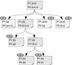
Figure 2.2: Representation of the agent’s search space at a particular time. Leaf nodes are active nodes which are matched againsts. The hashed nodes represent the search path along which generalisation and specialisation takes place. P. . .
represent the predicates describing the state.
As an example of the specialisation and generalisation process, figure 2.3 shows a possible path of expansion and retraction of nodes. For clarity, only the values of the nodes are depicted.
deleted and developed again so that a circle develops. To get back to a better expansion node can take a long time or even be almost impossible. To prevent such situations, it is possible to switch the search path. Although node values higher up in the tree might no longer be up-to date, the agent uses these values as a hypothesis that they are more promising than the current path. Switching happens with probability ρ,0 ≤ ρ ≤ 1, in which case the highest overall value in the tree is selected as the new expansion point. The path from the root to this node becomes thereby the search path.
Figure 2.4 illustrates the switching process. It shows that the result is similar to generalisation and specialisation. The difference is that the new path was not reachable because the deepest leaf nodes have a higher value than their (unchanged) parent. With the switching procedure, there is a chance that this trap is left.