Utilization of multi attribute decision making techniques to integrate automatic and manual ranking of options

Short Paper

__________________________________________________

Utilization of Multi Attribute Decision Making Techniques

to Integrate Automatic and Manual Ranking of Options

AMIN KARAMI1, 2_{AND RONNIE JOHANSSON}1,3

1_{School of Humanities and Informatics}

University of Skövde Skövde, 541 28 Sweden

2_{E-mail: [email protected];} 3_{[email protected]}

An information fusion system with local sensors sometimes requires the capability to represent the temporal changes of uncertain sensory information in dynamic and un-certain situation to access to a hypothesis node which cannot be observed directly. One of the central issue and challenging problem is the decision of what combination and or-der of sensors allocation should be selected between sensors, in oror-der to maximize the global gain in the flow of information, when the data association is limited. In this area, Bayesian Networks (BNs) can constitute a coherent fusion structure and introduce dif-ferent options (the combination of sensors allocation) for achieving to the hypothesis node through a number of intermediate nodes that are interrelated by cause and effect. BNs can rank the options in terms of their probabilities from Bayes’ theorem calculation. But, decision making based on probabilities and numerical representations might not be appropriate. Thus, re-ranking the set of options based on multiple criteria such as those of multi-criteria decision aid (MCDA) should be ideally considered. Re-ranking and se-lecting the appropriate options are considered as a multi-attribute decision making (MADM) problem by user interaction as semi-automatically decision support. In this paper, Multi Attribute Decision Making (MADM) techniques as TOPSIS, SAW, and Mixed (Rank Average) for decision-making as well as AHP and Entropy for obtaining the weights of attributes have been used. Since MADM techniques give most probably different results according to different approaches and assumptions in the same problem, statistical analysis done on them. According to the results, the correlation between com-pared techniques for re-ranking BN options is strong and positive because of the close proximity of weights suggested by AHP and Entropy. Mixed method as compared to TOPSIS and SAW is the preferred technique when there is no historical (real) deci-sion-making case; moreover, AHP is more acceptable than Entropy for weighting. Keywords: Bayesian networks, sensor allocation, TOPSIS, SAW, AHP, entropy

1. INTRODUCTION

There are different definitions of information fusion. One is that [1] “Information fusion is the study of efficient methods for automatically or semi-automatically trans- forming information from different sources and different points in time into a represen- tation that provides effective support for human or automated decision making.” One

technique for information fusion is Bayesian Networks (BNs) [2] which present know- ledge about domain variables in uncertain and unpredictable environments through nu- merical and graphical representation. Moreover, a Bayesian Network can constitute a coherent fusion structure with the hypothesis node which cannot be observed directly and sensors through a number of intermediate nodes that are interrelated by cause and effect. To be able to handle the uncertainty of sensor readings, information variables may add an additional layer of variables which connects sensors to hypothesis variables. In a target tracking case with the set of stationary sensors for observation of a hypothesis variable (node), number of participated sensors and select the appropriate option (different combination of sensors allocation) in the decision-making is a challenging problem [2]. Thus, it is important to present the better picture of sensor configuration options (both ranking and selecting) which are more useful in order to help decision makers for their decisions making [3]. Bayesian Networks provide important support for decision-making by ranking the set of options according to probabilities and numerical representations. But in some situations we need to make decision and rank or re-rank the set of options based on multiple criteria such as those of multi-criteria decision aid (MCDA) [4]. Bayesian theory provides inference mechanisms through subsets of evidence from inter- mediate variables to observe hypothesis (goal) nodes which are not directly observed [5]. Hence, the BN tool assists the intelligence analyst with analyzing incoming obser- vations. But in order to improve the results of the BN, we need to control sensors (to control the flow of information into the system) and for that purpose we consider sensor (configuration) options. Obviously, by user interaction, we can manage different possible options based on multi-criteria as semi-automatically Decision Support System (DSS). Multi-criteria analysis tries to incorporate multiple and different types of information and human experience into a DSS. Integration of human expertise with a fusion-based DSS can enable suggestions and recommendations for actions through understanding of pro- blems and problem solving skills within a specific domain [6]. Hence, re-ranking of options in Bayesian Network-based systems for achieving to a hypothesis/unobserved variable in terms of qualitative and quantitative criteria is one of the decision-making problems.

The rest of this paper is organized as follows. Section 2 presents related works. Multi-attribute decision-making (MADM) techniques are described in section 3. In sec-tion 4, Bayesian Networks and sensor allocasec-tion are reviewed. Experimental results are in detail in section 5. Finally, a conclusion is given in section 6.

2. RELATED WORKS

Using MADM techniques for improving decision making results are not a novel idea. There are several researches using MADM such as, TOPSIS [8, 29, 30], SAW [14, 29, 30], AHP [7, 10, 19, 31], and Entropy [20]. To the best of the author’s knowledge, there is no any applied MADM techniques for ranking and selecting the different com-bination of sensors allocation. Bayesian Network models are powerful tools for reason-ing and decision-makreason-ing under uncertainty, but BNs can provide different options of sensors allocation in terms of their probabilities from Bayes’ theorem calculation in order to estimate state of a hypothesis node through informational (intermediate) nodes [5]. However, (re-)ranking the different combination of sensors allocation can be considered as a MADM problem.

There are significant specifications of SAW and TOPSIS methods which include applicability for large-scale decision problems, simplicity in concept and computation, and applicability for hierarchical multi-level attributes. Moreover, AHP method is suit-able when an attribute hierarchy has more than three levels [10]. This means that the overall goal of the problem is on the top level, multiple criteria which define alternatives in the middle level, and competing alternatives in the bottom level. So, in this study, two techniques as SAW and TOPSIS according to their ideal characteristics have been se-lected. Since different methods provide different results, decision-makers use more than one technique in important decisions. In order to overcome this problem, we have util-ized Mixed (Rank Average) method which obtain from average of applied techniques results [11]. Likewise, AHP and Entropy are two important weight methods which we have used for them. By three different techniques and two weight methods, we are faced with five different re-rankings as TOPSIS with AHP, TOPSIS with Entropy, SAW with AHP, SAW with Entropy, and Mixed method. Since MADM methods have different approaches and assumptions for ranking/selecting options in the same problem, it is likely that they yield different results [9]. Therefore, applied MADM methods have in-vestigated by statistical tests if these differences are significant. We have used Kendall’s tau-b factor, Spearman correlation coefficient, and Pearson correlation coefficient (be-cause our study is about ranking data and data are quantitative). All statistical tests are implemented by SPSS software.

3. MULTI-ATTRIBUTE DECISION-MAKING TECHNIQUES

MADM problem-solving techniques provides a paradox between selections of MADM methods [12]. These contradictions may come from differences in use of weights, the selection approach of the ‘best’ solution, objectives scaling and introduction of additional parameters [13].

3.1 SAW (Simple Additive Weighting)

SAW model or Scoring Method (SM) is most often used in multi-attribute decision- making techniques. To do this, the normalized value of the criteria for the alternatives must be multiplied with the weight of the criteria. Then, the best alternative with highest score is selected as the preferred alternative [14]. The analytical structure of the SAW method for N options and M attributes can be summarized as:

1

1, 2, ..., .

M i j ij

j

s w r i N







si: is the overall score of the ith alternative; rij: is the normalized rating of the ith

alterna-tive for the jth criterion which:

max ij ij i ij x r x

 for the benefit and 1/ max (1/ )

ij ij i ij x r x

 for the

cost criterion representing an element for the normalized matrix; xij: is an element of the

decision matrix, which represents the original value of the jth criterion of the ith alterna-tive; wj: is the importance (weight) of the jth criterion; N and M are the number of

alter-natives and criteria, respectively.

3.2 TOPSIS (Technique for Order Preference by Similarity to Ideal Solution)

TOPSIS technique is suggested by Yoon & Hwang in 1981 [15]. Based on the idea that the best alternative should have the shortest geometric distance from a positive ideal solution (the best possible) and the longest geometric distance from a negative ideal so-lution (the worst possible), TOPSIS method consists of the following steps:

(1) Normalize the decision matrix: the normalization of the decision matrix is done us-ing the below transformation for each nij:

2 1 ij ij _m ij i a n a  



Then, weights should be multiplied to normalized matrix. (2) Determine the positive and negative ideal alternatives:

A+ _{= {v}+

1, v+2, …, v+n} = {(maxiVij|jJ), (miniVij|jJ|i = 1, 2, …, m)} (3)

Positive attribute: the one which has the best attribute values (more is better).

A- = {v1, v2, …, vn} = {(miniVij|jJ), (maxiVij|jJ|i = 1, 2, …, m)} (4)

J = {j = 1, 2, ..., n | j for posistive attributes}

J = {j = 1, 2, ..., n | j for posistive attributes}

Vij is the weighted normalized matrix.

(3) Obtain the separation measure (based on Euclidean distance) of the existing alterna-tives from ideal and negative one [16]:

0.5 2

1

( ) ; 1, 2,...,

n

ij j i

j

d V V i m

   _  _  



( ) ; 1, 2,...,

n

ij j i

j

d V V i m



 

_  _ 





(4) Calculate the relative closeness to the ideal alternatives:

;0 1; 1, 2,...,

( )

i

i i

i i

d

cl cl i m

d d



 

 

   

 . (6)

(5) Rank the alternatives: based on the relative closeness to the ideal alternative, the higher cli+, the better is the alternative A_i.

3.3 AHP (Analytical Hierarchy Process)

AHP was proposed by Thomas L. Saaty in 1995 [17]. It is a popular MADM tech-nique and widely used, especially in military problems [18]. AHP reflects the natural behavior of human thinking. This technique examines the complex problems based on their interaction effects. The details of AHP procedure are described in [17, 19].

3.4 Mixed Method

Decision-makers usually use more than one decision-making technique in important decisions. Different decision-making techniques may provide different results according to their approaches and assumptions. In order to overcome to this problem, Mixed method as Rank Average Method is used. Since the Mixed method involves average of methods re-sults and their specifications, it can be an ideal method in some problems [11].

3.5 Entropy

Entropy is the one of the most important concepts in social science, physics, and in-formation theory. Shannon’s entropy method is suitable for finding the appropriate weight for each criterion in MADM problems [20]. According to this method, whatever disper-sion in the index is greater, the index is more important. Entropy steps are as follow:

Step 1: Calculate Pij to eliminate anomalies with different measurement units and scales.

1 ; ij ij m ij i a P j a   

Step 2: Calculate the entropy of Ej

1 1

[ ln ]; . ln( )

m

j ij ij

i

E P P j

m 

  

_{ } 

 



Step 3: Calculate of uncertainty dj as the degree of diversification

dj = 1 Ej; j. (9)

Step 4: Calculate of weights (Wj) as the degree of importance of attribute j

Wj = 1

; .

j n

j j

d j d







Where aij is value of ith option (entry) for jth index; Pij is the value-scale of jth index for

ith option (entry).

4. BAYESIAN NETWORKS AND SENSOR ALLOCATION

The sensor allocation problem has been considerably investigated in recent years. Two research issues of sensor allocation include deciding where to physically deploy sensors, and decide which physical parameters should be measured by sensors. Also, optimal sensor allocation is where to allocate sensor, which is closely related to deci-sion-making objectives. To do this, a Bayesian Network is built to represent the causal relationships between the observable variables in order to determine which observable variables should be sensed [21, 22]. Moreover, Bayesian Networks are used to find the prioritization of sensor options through value of obtained information from domain [23].

uncer-tainty of sensor readings in a Bayesian network, we can add an additional layer of vari-ables as ‘information varivari-ables’ which connect intermediate varivari-ables to sensors [2].

5. EXPERIMENTAL RESULTS

5.1 Identification of General Decision-Making Criteria

We have used literature review and recent experiences of some specialists in order to identify some general decision-making attributes (criteria) for re-ranking the BN options. Most criteria depend on three factors: Characteristics of the choice (e.g., uncertainty, complexity, and instability), Environment (e.g., time and resource available, irreversibility of the choice, and possibility of failure), and decision maker (e.g., knowledge, strategies, expertise, and motivation). In a Bayesian Network model, experts with different knowl-edge in a same project may have different solutions and opinions for identifying the causal relationship among variables, quantifying graphical models, and ranking on the set of op-tions in terms of numerical probabilities [25]. Moreover, a combination of contextual and informational decision factors will have effect on decision making [26]. These factors are politics, power structure, trust, and time pressure for rapid decisions. In addition, tangible factors include cost, risk, adherence to organizational technology standards and strategies, and informal external information sources with their relationship. In order to final identi-fication of general attributes, we have used Delphi method as a structured communication technique which relies on a panel of experts. Ten experts that were familiar with sensor allocation and Decision Support Systems concepts were chosen. After this procedure, the ten attributes as final general attributes were selected in Table 1.

5.2 Results and Discussion

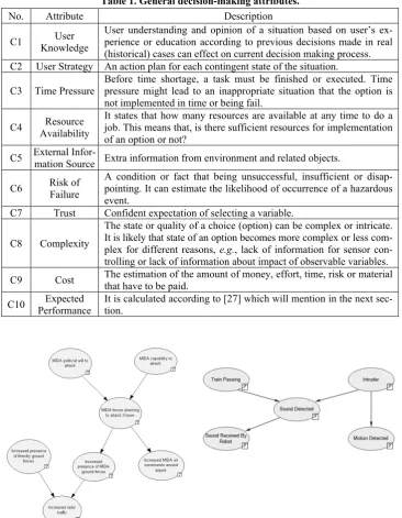
We conducted two experiments using two real scenarios (drawn with the GeNIe tool). We constructed 1st _{scenario of a fusion structure with a Bayesian Network from}

[27]. This BN (Fig. 1) includes a hypothesis variable (corresponding to a knowledge re-quest issued by an intelligence analyst and not directly observable) and information vari-ables. In this BN example, only “will to attack”, “capability to attack”, “increased air movements”, “increased radio”, and “increased presence of friendly” can be observed. The hypothesis variable as “planning to attack X-town” can normally not be observed. The variable “increased presence of MIDA” also has not been considered. In the 2nd

sce-nario (Fig. 2)1_{, there is a mobile robot acting as a night guard on the entrance floor of a}

small business building to find an intruder. In this example, “Motion Detected”, “Sound Received By Robot” (information variables), “Sound Detected”, “Train Passing” (medi-ating variables) can be observed, and the hypothesis variable is “Intruder”.

One method for acquiring information in general Bayesian Networks with uncertain observations has been proposed in [27]. They have enumerated all possible options (al-location of sensing resources to Bayesian Network variables) and evaluated them ac-cording to their expected impact if an option was implemented. The details of expected performance calculation are also described in [27].

Table 1. General decision-making attributes.

No. Attribute Description

C1 _Knowledge User User understanding and opinion of a situation based on user’s ex-perience or education according to previous decisions made in real (historical) cases can effect on current decision making process. C2 User Strategy An action plan for each contingent state of the situation.

C3 Time Pressure Before time shortage, a task must be finished or executed. Time pressure might lead to an inappropriate situation that the option is not implemented in time or being fail.

C4 _Availability Resource It states that how many resources are available at any time to do a job. This means that, is there sufficient resources for implementation of an option or not?

C5 External Infor-_{mation Source} Extra information from environment and related objects.

C6 Risk of Failure

A condition or fact that being unsuccessful, insufficient or disap-pointing. It can estimate the likelihood of occurrence of a hazardous event.

C7 Trust Confident expectation of selecting a variable.

C8 Complexity

The state or quality of a choice (option) can be complex or intricate. It is likely that state of an option becomes more complex or less com-plex for different reasons, e.g., lack of information for sensor con-trolling or lack of information about impact of observable variables. C9 Cost The estimation of the amount of money, effort, time, risk or material _{that have to be paid.}

C10 _Performance Expected It is calculated according to [27] which will mention in the next sec-_tion.

Fig. 1. MIDA scenario [27]. Fig. 2. Mobile robot scenario.

ex-pert users as well as analysis and comparison. The reason of using the expected per-formance is that, it was the only appreciable and available criterion from investigated options. In the first scenario, the structure of every option is, e.g., ((2, 1, 1, 0, 0), 0.9939219115):

 1st Number: 2 sensors/resources were assigned to the attack_will variable,

 2nd Number: 1 sensor to attack_capability,

 3rd Number: 1 sensor to air_movements,

 4th Number: 0 sensor to presence_friendly,

 5th Number: 0 sensor to radio_traffic, and

 6th Number: 0.9939219115 is expected performance.

In the second scenario, the structure of every option is, e.g., ((3, 1, 0, 1), 0.9949520805):

 1st Number: 3 sensors/resources were assigned to the MotionDetected variable,

 2nd Number: 1 sensor to SoundReceivedByRobot,

 3rd Number: 0 sensor to SoundDetected,

 4th Number: 1 sensor to TrainPassing, and

 5th Number: 0.9949520805 is expected performance.

As main problem is re-ranking of these generated options (different combination of sensors allocation), we are going to re-rank these options via Multi Attribute Decision Making (MADM) techniques by user interaction. For filling the decision matrix with 20 options and 10 attributes (criteria), we employ the experiences of three expert users in military sections (meaning with extended experience in the application of information fusion and Bayesian Networks systems) in two scenarios (Figs. 1 and 2).

Analysis of decision matrix should be included quantitative values, but some criteria were qualitative. Hence, Odd Bipolar Scaling is used to convert qualitative variables to quantitative. Since scales of attributes measurement are different, they should be expressed as non-scaling values. To do this, linear non-scaling method used as follow:

For positive attributes: max

ij i ij

r

r and for negative attributes:

1/ max (1/ )

ij i ij

r

r where, rij is the

value of ith row and jth column and maxi is maximum value of ith column.

Table 2. Attributes weight by AHP technique.

Attributes Weight Attributes Weight

(1) User strategy 0.234 (6) Trust 0.066

(2) Cost 0.196 (7) Expected Performance 0.046

(3) Resource Availability 0.128 (8) External Information Sources 0.044

(4) User Knowledge 0.124 (9) Possibility of Failure 0.027

(5) Time Pressure 0.109 (10) Complexity 0.026

To do TOPSIS, after multiplying weights (from AHP) to normalized matrix (Eq. (2)), we should determine the positive and negative ideal alternatives (Eqs. (3) and (4)):

Table 3. Positive and negative ideal alternatives with TOPSIS-AHP.

A+ 0.04838 0.04083 0.00690 0.02084 0.01297 0.01637 0.07700 0.00298 0.00208 0.01609

A- 0.00537 0.00453 0.06211 0.00231 0.00144 0.14736 0.00855 0.00894 0.01875 0.00566

Then, we should calculate Euclidean distance of alternatives (Eq. (5)):

Table 4. Euclidean Distance in TOPSIS-AHP.

Options di+ d_i- Options d_i+ d_i

-O1 0.04568 0.14525 O11 0.07268 0.14783

O2 0.04217 0.14850 O12 0.07095 0.12059

O3 0.08483 0.12064 O13 0.07061 0.11896

O4 0.03237 0.14987 O14 0.04781 0.14424

O5 0.05150 0.15497 O15 0.08032 0.11885

O6 0.05426 0.14488 O16 0.04481 0.15295

O7 0.13919 0.07335 O17 0.03895 0.15750

O8 0.04344 0.15558 O18 0.08343 0.13857

O9 0.03882 0.15292 O19 0.03913 0.15032

O10 0.04740 0.13778 O20 0.08815 0.13851

Finally, calculating the relative closeness to the ideal alternatives and ranking the alter-natives based on cli+ (Eq. (6)):

Table 5. Rank the alternatives with TOPSIS-AHP.

Options cli+ Re-ranking Options cl_i+ Re-ranking

O1 0.76073 8 O11 0.67040 13

O2 0.77885 6 O12 0.62957 14

O3 0.58715 19 O13 0.62753 15

O4 0.82239 1 O14 0.75106 9

O5 0.75055 10 O15 0.59674 18

O6 0.72751 12 O16 0.77339 7

O7 0.34511 20 O17 0.80172 2

O8 0.78173 5 O18 0.62418 16

O9 0.79755 3 O19 0.79347 4

Re-ranking results from applied methods are shown in Figs. 3 and 4. The obtained re-ranking results from five different techniques are very different as compared to rank-ing only based on the expected performance. This means that, by user interaction we could evaluate every twenty options with ten criteria as semi-automatically decision support. For example in Fig. 3, first, second, third, and fourth options in initial ranking have been changed to seventh, eleventh, fifteenth, and sixth ranked in average re-ranking. Hence, the first five best options regarding to user interaction are ninth, nineteenth, sev-enteenth, eighth, and fifth options. In Fig. 4, 1st_{, 2}nd_{, 3}rd_{, and 4}th _{options in first ranking}

have changed to 14th_{, 8}th_{, 15}th_{, and 5}th _{in average re-ranking, respectively. In contrast,}

first four options in average re-ranking have become options of 17th_{, 9}th_{, 19}th_{, and 8}th_,

respectively. In spite of obtained different results from five techniques, we cannot con-clude which one is better and more acceptable than others. Because we need to investi-gate and evaluate these results with some historical real cases. Obviously, previous deci-sions made are helpful to evaluate which techniques are more close to real decideci-sions and which ones are not. In the duration of the evaluation of experimental results, it was diffi-cult to get real cases (either the military is not willing to share or they do not have time). In order to do the evaluation properly, we would have to set up practical experiments with domain experts and show that the joint decision making (fusion system and hu-man-based MADM) is more efficient than either of the two independently. Hence, in the absence of historical decisions made, analysis of the integration (or usage) of MADM with BNs results can improve decision-making performance by incorporating experi-ences and knowledge of decision makers (experts) as a semi-automatically decision- making system. According to Fig. 3, trend of variations in five applied techniques are similar. For instance, fourth option as the highest variation is ranked to 1st_{, 5}th_{, 6}th_{, 9}th_,

and 11th _{from TOPSIS (AHP), SAW (AHP), Mixed, TOPSIS (Entropy), and SAW}

(En-tropy), respectively. In contrast, ninth option as one of the lowest variation is ranked to 3rd _{from TOPSIS (AHP) and 1}st _{from four other techniques. Moreover, in Fig. 4, first}

option as the highest variation is ranked to 11th_{, 7}th_{, 13}th_{, 9}th_{, and 14}th _{from SAW (AHP),}

SAW (Entropy), TOPSIS (AHP), TOPSIS (Entropy), and Mixed, respectively. In con-trast, fourth option as one of the lowest variation is ranked to 11th _{from SAW (AHP), 9}th

from SAW (Entropy), and 5th _{from three other techniques. Comparison of results via}

sta-tistical tests can be helpful in order to define which method can be preferred among oth-ers, when there is no any historical case (decision made). Because statistical tests can be employed for obtaining the strong correlation and relationship between different results in applied techniques.

5.3 Comparison of Results

Fig. 3. Results of the rank from five applied techniques in 1st _scenario.

Fig. 4. Results of the rank from five applied techniques in 2nd _scenario.

Table 6. Results of Pearson, Spearman and Kendall’s TAU-B correlation.

1st _{Scenario 2}nd_Scenario

Pearson and Spearman

Correlation Kendall's TAU-B Correla-tion Pearson and Spearman Correlation Kendall's TAU-B Correla-tion

Paired

Com-parison Correlation Coefficient Comparison Paired Correlation Coefficient Paired Compari-son Correlation Coefficient Paired Com-parison Correlation Coefficient

SAW (AHP)

Mixed 0.950 SAW (AHP) Mixed 0.821 TOPSIS (AHP)Mixed 0.962 TOPSIS (AHP) Mixed 0.889 SAW (Ent.)

Mixed 0.913 SAW (Ent.) Mixed 0.768 SAW (AHP) Mixed 0.933 TOPSIS (Ent.) Mixed 0.818 SAW (AHP)

TOPSIS (AHP) 0.913 TOPSIS (Ent.)Mixed 0.758 TOPSIS (AHP)SAW (AHP) 0.911 SAW (Ent.) Mixed 0.775 TOPSIS (AHP)

Mixed 0.899

TOPSIS (AHP) SAW (AHP) 0.747

SAW (Ent.)

Mixed 0.901

TOPSIS (AHP) SAW (AHP) 0.755 TOPSIS (Ent.)

Mixed 0.893 TOPSIS (AHP)Mixed 0.716 TOPSIS (Ent.) Mixed 0.90 SAW (AHP) Mixed 0.749 SAW (AHP)

SAW (Ent.) 0.851 SAW (AHP) SAW (Ent.) 0.674 TOPSIS (AHP) SAW (Ent.) 0.882 TOPSIS (Ent.) SAW (AHP) 0.711 SAW (Ent.)

TOPSIS (Ent.) 0.851

SAW (Ent.)

TOPSIS (Ent.) 0.674

SAW (Ent.)

TOPSIS (Ent.) 0.861

TOPSIS (AHP) SAW (Ent.) 0.694 SAW (AHP)

TOPSIS (Ent.) 0.737 TOPSIS (Ent.)SAW (AHP) 0.579 TOPSIS (AHP) TOPSIS (Ent.) 0.802 SAW (AHP) SAW (Ent.) 0.621 TOPSIS (AHP)

TOPSIS (Ent.) 0.735 TOPSIS (AHP) TOPSIS (Ent.) 0.537 TOPSIS (Ent.) SAW (AHP) 0.774 TOPSIS (AHP) TOPSIS (Ent.) 0.587 TOPSIS (AHP)

Since there is much data (20 entries), the results of Pearson and Spearman are convergent (Table 6). According to Table 6, the correlation between different applied techniques with 99% of confidence level is strong and positive which is statistically significant (p < 0.01). This very high confidence level comes from statistical tests output in SPSS software as ‘correlation is significant at the 0.01 level (2-tailed)’. In both scenarios, the correlation between TOPSIS and SAW techniques with AHP method (0.913 and 0.911) is stronger than with Entropy method (0.851 and 0.861). Moreover, correlation between TOPSIS, SAW, and Mixed (0.899 and 0.95 in 1st _{scenario, 0.962 and}

0.933 in 2nd _{scenario) with AHP are better than with Entropy (0.893 and 0.913 in 1}st

scenario, 0.9 and 0.901 in 2nd _{scenario). Significant statistical correlation between ranked}

options with five different techniques is because of the close proximity of weights by AHP and Entropy. In the Table 6, the highest relation is Mixed method with SAW and TOPSIS by both AHP and Entropy. Since the Mixed method involves average of methods results, it is expected to have a stronger correlation as compared to others. When there is no historical real case for investigation of correlation between real decisions made and applied techniques, Mixed method can be ideal technique among others. In contrast, the almost lowest relation is TOPSIS (AHP) with SAW (Entropy) and TOPSIS (Entropy) with SAW (AHP). Hence, Mixed method has provided better results with the most correlations among other paired comparisons. The values for concordance coefficient from Kendall’s tau_b results are close to +1; as a result, there is a large agreement between the ranks. Also, concordance coefficient between applied techniques with AHP is better than Entropy.

6. CONCLUSION

REFERENCES

1. H. Boström, S. F. Andler, M. Brohede, R. Johansson, A. Karlsson, J. van Laere, L. Niklasson, M. Nilsson, A. Persson, and T. Ziemke, “On the definition of information fusion as a field of research,” Technical Report, HS-IKI-TR-07-006, School of Hu-manities and Informatics, University of Skövde, Sweden, 2007.

2. T. J. Stevens and M. K. Sundareshan, “Probabilistic neural network-based sensor configuration management in a wireless ad-hoc network,” Department of Electrical and Computer Engineering, University of Arizona, Tucson, 2004.

3. E. Bossé, J. Roy, and S. Wark, Concepts, Models, and Tools for Information Fusion, Artech House Inc., Norwood, MA, 2007.

4. N. Fenton and M. Neil, “Making decisions: using Bayesian nets and MCDA,” Know-

ledge-Based Systems, Vol. 14, 2001, pp. 307-325.

5. E. Besada-Portas, J. A. Lopez-Orozco, and J. M. de la Cruze, “Unified fusion system based on Bayesian networks for autonomous mobile robots,” in Proceedings of the 5th International Conference on Information Fusion, 2002, pp. 873-880. 6. M. Nilsson and T. Ziemke, “Information fusion: A decision support perspective,” in

Proceedings of the International Conference on Information Fusion, 2007, pp. 1-8.

7. M. Pirdashti, A. Ghadi, M. Mohammadi, and G. Shojatalab, “Multi-criteria decision- making selection model with application to chemical engineering management deci-sions,” in Proceedings of World Academy of Science, Engineering and Technology, Vol. 49, 2009, pp. _____.

8. K. Devi, S. P. Yadav, and S. Kumar, “Extension of fuzzy TOPSIS method based on vague sets,” Computational Cognition, Vol. 7, 2009, pp. 58-62.

9. S. K. Cheng, “Development of a fuzzy multi-criteria decision support system for municipal solid waste management,” Master Thesis, Applied Science in Advanced Manufacturing and Production Systems, University of Regina, Canada, 2000. 10. C. Yeh, “A problem-based selection of multi-attribute decision making methods,”

International Transactions in Operational Research, Vol. 9, 2002, pp. 169-181. 11. H. Soltanpanah, H. Farughi, and M. Golabi, “Utilization and comparison of multi at-

tribute decision techniques to rank countries upon human development rate,” Inter-national Research Journal of Finance and Economics, Issue 60, 2010, pp. 175-188. 12. E. Triantaphyllou, Multi-attribute Decision Making Methods: A Comparative Study,

Kluwer Academic Publishers, ____(place), 2000.

13. J. Lezzi, “Multi-criteria decision making in outpatient scheduling,” Master Thesis, Department of __________, University of South Florida, USA, 2006.

14. M. Janic and A. Reggiani, “An application of the multiple criteria decision making (MCDM) analysis to the selection of a new hub airport,” European Journal of Transport and Infrastructure Research, Vol. 2, 2002, pp. 113-142.

15. K. Yoon and C. L. Hwang, Multiple Attribute Decision Making Methods and Appli-cations, Springer Verlag, ____(place), 1981.

16. L. Jorge, A. García, M. G. Ibarra, and P. L. Rico, “Improvement of TOPSIS tech-nique through integration of Malahanobis distance: A case study,” in Proceedings of

the 14th Annual International Conference on Industrial Engineering Theory,

Appli-cations and Practice, 2009, pp. 135-141.

18. G. Coyle, The Analytic Hierarchy Process (AHP), Practical Strategy, Open Access

Material, Pearson Education Limited, 2004.

19. H. Ariff, M. S. Salit, N. Ismail, and Y. Nukman, “Use of analytical hierarchy process (AHP) for selecting the best design concept,” Jurnal Teknologi, Vol. 49(A) Dis., 2008, pp. 1-18.

20. M. E. Andreica, I. Dobre, M. I. Andreica, and C. Resteanu, “A new portfolio selec-tion method based on interval data,” Studies in Informatics and Control, Vol. 19, 2010, pp. 253-262.

21. W. Watthayu and Y. Peng, “A Bayesian network based framework for multi-criteria decision making,” in Proceedings of the 17th International Conference on Multiple Criteria Decision Analysis, 2004, pp. ______.

22. J. Li and J. Jin, “Optimal sensor allocation by integrating causal models and set- covering algorithms,” IIE Transactions, Vol. 42, 2010, pp. 564-576.

23. F. Jensen, Bayesian Networks and Decision Graphs, Springer-Verlag, ____(place), 2002.

24. F. Saidi, O. Stasse, and K. Yokoi, “A visual attention framework for search behavior by a humanoid robot,” in Proceedings of the 6th IEEE-RAS International Confer-ence on Humanoid Robots, 2006, pp. 346-351.

25. W. Premchaiswadi and N. Jongsawat, “Group decision making using Bayesian net-work inference with qualitative expert knowledge,” in Proceedings of the 5th IEEE International Conference on Intelligent Systems, 2010, pp. 126-131.

26. J. Jamieson, “Information systems decision making: factors affecting decision mak-ers and outcomes,” Ph.D. Thesis, Department of Business and Informatics, Central Queensland University Rockhampton, Australia, 2007.

27. R. Johansson and C. Martenson, “Information acquisition strategies for Bayesian net- work-based decision support,” in Proceedings of the 13th International Conference on Information Fusion, 2010, pp. 1-8.

28. G. A. Mendoza, P. Macoun, R. Prabhu, D. Sukadri, H. Purnomo, and H. Hartanto,

Guidelines for Applying Multi-Criteria Analysis to the Assessment of Criteria and Indicators, Center for International Forestry Research, Jakarta.

29. R. Simanaviciene and L. Ustinovichius, “Sensitivity analysis for quantitative deci-sion making methods: TOPSIS and SAW,” in Proceedings of the16th International

Conference on Information and Software Technologies, 2010, pp. ______.

30. E. Stevens-Navarro and V. W. S. Wong, “Comparison between vertical handoff de-cision algorithms for heterogeneous wireless networks,” in Proceedings of the 63rd

IEEE Vehicular Technology Conference, Vol. 2, 2006, pp. 947-951.

31. A. P. Agalgaonkar, S. V. Kulkarni, and S. A. Khaparde, “Multi-attribute decision making approach for strategic planning of DGs,” IEEE Power Engineering Society General Meeting, 2005, pp. 2985-2990.