item and our policy information available from the repository home page for further information.
Author(s): Pedersen, Jacob L.; Dodds, Stephen J.
Title: Forced dynamic control of non-minimum-phase plants via study of the classical inverted pendulum
Year of publication: 2010
FORCED DYNAMIC CONTROL OF NON-MINIMUM-PHASE
PLANTS VIA STUDY OF THE CLASSICAL INVERTED
PENDULUM
Jacob L. Pedersen†, Stephen J. Dodds‡
†Delphi Diesel Systems Ltd, Park Royal, London, United Kingdom ‡CITE, University of East London, United Kingdom
[email protected], [email protected]
Abstract: The general problem of controlling a non-minimum-phase plant is tackled via study of the classical inverted pendulum (IP). A full nonlinear model of the IP is used for simulation and a linearised version is used for the controller design. The trolley position is controlled while keeping the pendulum inverted by use of an input/output feedback linearisation method called Forced Dynamic Control (FDC). This is generally more straightforward to apply than conventional techniques such as linear state feedback with pole assignment but in its basic form yields right half plane zero cancellation which creates an unstable closed loop mode. This is circumvented in this paper by creating an artificial controlled output that is a weighted sum of the state variables such that the right half plane zeros do not exist in the transfer function. Furthermore a non-oscillatory response with a specified settling time is achieved with the aid of the Dodds settling time formula (Dodds, 2008). The computational delay introduced to eliminate the algebraic loop in the nonlinear model is shown to have a negligible effect. Simulations are presented that demonstrate the correct operation of the control system and determine differences between the ideal and actual step responses due to the nonlinearities, parametric errors and external disturbances.
1. Introduction
It is well known that linear state feedback control (LSFC) laws for linear non-minimum phase plants, can be designed by pole assignment, an acceptable transient response being attainable by balancing the right half plane zeros by mirror image poles (Franklin et al., 2002). This is applicable, for example, to the inverted pendulum when its motion is restricted to small perturbations about an operating point. The motivation for applying forced dynamic control (FDC), however, is that it is also applicable to nonlinear plants and is quicker to apply than conventional LSFC. Since FDC is a time domain method, a different approach to deal with non-minimum phase plants is needed. It should be noted here that the term ‗non-minimum phase‘, strictly
applies to linear plants and that the equivalent term covering nonlinear plants in addition is ‗unstable zero dynamics‘ (Stadler, 2008). The direct application of FDC to a plant of rank r n where n is the plant order will leave the zero dynamics of order n r uncontrolled in the closed loop system. The purpose of this paper is to investigate the solution of this problem by appending the plant state space model with an artificial output equation such that the ‗new plant‘ created is of full rank and the application of FDC to this achieves full state control and therefore avoids the closed loop instability. The paper addresses the choice of the closed loop dynamics using the Dodds settling time formula (Dodds, 2008).
performance of this design is assessed for the true nonlinear IP as well as the linearised model by simulation. It is intended that the work presented here should pave the way to generally applicable FDC of plants with unstable zero dynamics.
2. Inverted pendulum modelling
2.1 Nonlinear model
The input force, F, is used for controlling the movement of the IP, as shown in Figure 11.
Trolley
0 X
Y
F
xP
xT
yP
l m , J
P
yT Pivot point
Trolley mass = M
Figure 11 Inverted pendulum system
The coordinates, θ (angle of the pendulum) and xT (position of the trolley), are outputs
from the single input, multiple output (SIMO) plant.
Lagrange‘s method is used to derive the following equations of motion:
2
cos sin
T T
F b x ml ml
x
M m (1)
2
sin Tcos
mgl ml x
m l J (2)
2.2 Linear IP model
Linearising (1) and (2) about the operating point, 0yields:
1
T T
b m l
x x F
M m M m M m (3)
2 2 T
mgl ml
x
J l m J l m (4)
The states of the IP are chosen as x1 ,
2
x , x3 xT and x4 xT. Equations (3) and (4) may then be replaced by the following state differential equation:
x A x B u
1 1
0 1
2 2 0
3 3
2 3
4 4 1
0 1 0 0 0
0 0
0 0 0 1 0
0 0
x x
a a
x x b
F
x x
a a
x x b
(5)
The measurement equation is
y C x
1
2
3
4
1 0 0 0
0 0 1 0
T
x
x
x x
x
(6)
where
0 1
a M m m g l q ,a1 m l b q1,
2
2 2
2
a m g l q , a3 J l2 m b q2,
0 1
b m l q , b1 J l2 m q2 and
2 1
q J M m l M m,
2 2
q J M m l m M
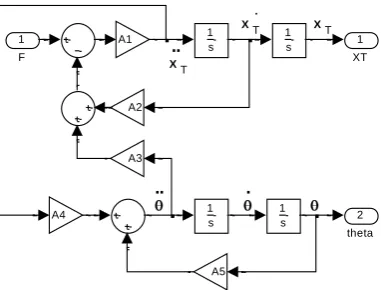
. .. XT X . T X T .. 2 theta 1 XT 1 s 1 s 1 s 1 s A4 A1 A3 A5 A2 1 F
Figure 12: Linear IP Simulink model
3. Forced Dynamic Control (FDC)
The general FDC method is fully described by (Vittek and Dodds, 2003). Here, the goal is to control the trolley position while keeping deviations of the pendulum position about the vertical within acceptable bounds. It is evident by inspection of (1) and (2) that this plant is of order, 4. The rank w.r.t. the controlled output, xT, is 2 due to the direct
dependence of xT on the control force, F.
Direct application of FDC would therefore yield a closed loop system of order 2 and therefore only two of the plant state variables, i.e., xT and xT, would be
controlled. The other two state variables, and , are associated with the zero dynamic subsystem (2). The input of this subsystem is xT but this is not used to control the
pendulum angle, , which will vary as a ‗side effect‘. In the linearised model, the zero dynamics is described by (4) and the natural motion of the unforced system, obtained by setting xT 0, is unstable since the roots of the characteristic equation,
2 2
0
s mgl J l m are s1,2 mgl J l m2 .
To circumvent this problem, the approach taken is to augment the plant model by creating an artificial controlled output
1 T 2 T 3 4
z C x C x C C (7)
where the constant coefficients are chosen such that a) the plant is of full rank, i.e., the rank with respect to z is 4, and b) controlling z to reach a constant demanded value results in xT reaching the same value. Figure 13
shows a block diagram of this augmented plant. For conciseness, the coefficients are defined as A1 1 M m , A2 b, A3 ml,
2 4
A ml J l m and A5 mgl J l m2 .
The standard FDC method will now be applied to the augmented plant of Figure 13. Since the plant has to be of full rank, C1, C2,
C3 and C4 are chosen so that z, z, and zz
are state variables, which is achieved by
[image:4.595.86.277.111.256.2]. .. XT X . T XT .. 1 Z 1 s 1 s 1 s 1 s C4 C3 C2 C1 A4 A1 A3 A5 A2 1 F
Figure 13: Linear IP with artificial output z.
ensuring that none of these variables has direct algebraic dependence on the control variablrale, F. Differentiating (7) yields
1 T 2 T 3 4
z C x C x C C (8)
Substituting for the derivatives of the state variables appearing on the right hand side of (8) using (5) and (6) yields:
1 T 3 2 1 2 T 3 4
z C x C C A F A x A C (9)
From Figure 13,
5 4 1 2 T 3
A A A F A x A
4 1 3 5 4 1 4 1 2
1 A A A A A A F A A A xT
5 4 1 4 1 2 T 1 4 1 3
Substituting for in (9) using (10) yields
1 3 2 1 2 1 2
5 4 1 4 1 2
4 2 1 3
4 1 3
1
T T
T
z C x C C A F C A A x
A A A F A A A x C C A A
A A A
. (11)
The F term in (11) must vanish in order for
zto be a state variable. Hence C4 C A A2 1 3 and C2 0 C4 0 which yields
1 T 3
z C x C z C x1 T C3 . (12)
Repeated substitution for xT and using
the equations implied by Figure 13 yields
1 1 2 3
3 5 4 1 2 3
T
T
z C A F A x A
C A A A F A x A
1 3 4 1 2 T 3 3 5
z C C A A F A x A C A
3 5
2
1 3 4 1 5 4 1 4 1 2 3
4 1 3
1 T
T
z C A
F A x
C C A A A A A F A A A x A
A A A
(13)
For F to vanish, C1 C A3 4, yielding
3 5
z C A and differentiating again yields
3 5
z C A . (14)
3
C has be chosen such that z xT in the steady state assuming closed loop stability. Then, xT const, xT 0, 0 and 0
and therefore the steady state outputs satisfy
1 ss 1 1 3 1 4
ss T
z C x C C A .
Summarising, the required constants are C1 1,
2 0
C , C3 1 A4 and C4 0. Then (7) yields
1 T 3 T 1 4
z C x C x A (15)
4
1
T
z x A (16)
5 4
z A A (17)
5 4
z A A (18)
The output derivative equation for FDC is then obtained by a further differentiation:
3 5
z C A
Substituting for using (10) yields
5 4 1 4 1 2
3 5
4 1 3
1
T
A A A F A A A x
z C A
A A A
5 5 4 1 4 1 2
4 1 4 1 3
T
A A A A F A A A x
z
A A A A
Solving for F then yields the general FDC law in which z has to be chosen to achieve the required closed loop dynamics:
4
4 1 3 4 1 5
5 4 1 2
1
1
T
A
F A A A z
A A A
A A A A x
(19)
The Dodds 5% settling time formula, 1.5 1
s c
T n T (Dodds, 2008), will now be used to obtain the desired non-overshooting closed loop step response, z t . Thus
1.5 1 1
1 1.5 1
n n C S r C S n
z s T T
n
z s s
s
T T
(20)
Where zr is the reference input and Tc is
closed-loop time constant for the n-order system. For n = 4, (18) becomes
4
r
z s a
z s s a where
15 2 S
a T from which
4 3 2 2 3 4 4
4 6 4 r
s as a s a s a z s a z s
so in the time domain:
2 3 4 4
4 6 4 r
z a z a z a z a a z
4 3 2
4 6 4
r
z a z z a z a z a z
Using (13) to (16) and setting
r
r T
4 3
4 4
2 5 5
4 4
1 1
4
6 4
Tr T T
z a x x a x
A A
A A
a a
A A
(21)
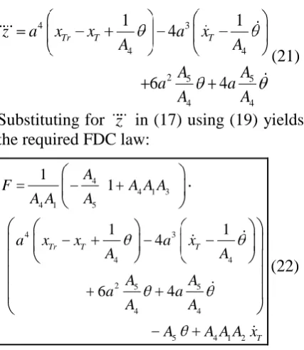
Substituting for z in (17) using (19) yields the required FDC law:
4
4 1 3
4 1 5
4 3
4 4
2 5 5
4 4
5 4 1 2
1
1
1 1
4
6 4
Tr T T
T
A
F A A A
A A A
a x x a x
A A
A A
a a
A A
A A A A x (22)
To summarise, an overall block diagram of the control system is shown in Figure 4.
Forced dynamic control (FDC) F Tr x Reference input:
IP plant / plant model
, ,xT,xT
Trolley 0 X Y F xP xT
yP l m , J P
yT Pivot point Trolley mass = M
States:
Figure 14: FDC and IP plant
Regarding future practical implementation, a rapid prototyping system such as dSPACE could be used. All the plant states are required but in the real world only the trolley position
T
x and the pendulum angle would be
measured. The other states, xT and could be calculated using software differentiation. As formulated above, the control variable is the force F [Nm] but in the real system this would be implemented as a control signal equivalent to the force from the processor. For example, if the actuator is a DC motor, the torque would be m K im a R F r. where
a
i is the armature current, Km is the motor
torque constant, R is the gearbox ratio and r
is the truck wheel radius from which .
a m
i R r K F. This would then be the
current demand of a relatively high bandwidth current control loop as shown in Figure 15.
DC motor F Closed loop current control ia Force equivalent current (from the FDC)
[image:6.595.74.288.105.351.2]Gearbox & wheels m
Figure 15: Control force implementation.
4. Simulations
Parameters:
The parameters used are as follows unless otherwise specified: Gravitational acceleration:
2
9.8 sec
g m ; Trolley mass: M 0.4 kg ;
Pendulum mass: m 0.1 kg ; Pendulum
length: l 0.5 m ; Moment of inertia about
the pendulums pivot point: 2 2
3 kg
J ml m .
Simulations with linear plant model:
In all the simulations presented below, all the state variables start at zero, the 5% settling time is set to Ts 2 s, a positive step
truck position reference,
r
T
x t is applied at
2s
t and an equal and opposite step reference input is applied at t 7 s.
the response to two consecutive oppositely signed steps of 1m magnitude of the FDC applied to the aforementioned model superimposed on the step response of the nominal closed loop system with transfer function (18) for n 4, which is used as a benchmark. These responses are not distinguishable from one another and pass through the 0.95
r
T
x line at t Ts 2 s,
[image:7.595.308.508.175.340.2]confirming their correctness.
Figure 16: Validation of FDC
As no error between the two responses is visible in Figure 16, Figure 17 shows this error on a visible scale, proving that it is negligible. The pseudo random behaviour is due to the numerical integration operating at a finite word-length.
Figure 17: Error between z of simulated FDC without the plant delay and nominal z.
Figure 18 shows the corresponding trolley position, indicating the undershoot following the step changes in
r
T
x that are
typical with non-minimum-phase plants.
Figure 18 Trolley position
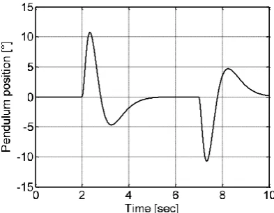
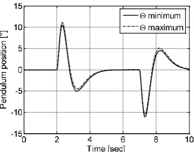
At less than 10%, of the step reference input magnitude, this undershoot is considered to be acceptable. The corresponding pendulum angle plotted in Figure 19 is kept within
11deg. of the vertical position, confirming the effective control of all the plant states.
Figure 19: Pendulum position (Vertical = 0)
Figure 20 shows the error corresponding to Figure 19 when the plant model without the algebraic loop (Figure A1 in the Appendix to this paper) is replaced by the basic one of Figure 12 but with a time delay of h 1ms introduced
between and the gain, A3. Although this has
[image:7.595.74.273.263.418.2] [image:7.595.310.507.442.595.2] [image:7.595.81.273.536.693.2]approximately1011, the peak error is less than
4
[image:8.595.76.274.169.332.2]10 m in magnitude, which can be considered acceptable when compared with the position change of 1 m.
Figure 20 Error between z of simulated FDC with the plant delay and nominal z.
Simulations with nonlinear plant model:
Figure 21 shows a step response error corresponding to Figure 20 but with the nonlinear plant model using the same FDC control law as applied above to the linear plant model.
Figure 21: Error between nominal z and z of FDC with nonlinear plant model and delay.
As can be seen, the error increases further in magnitude by a factor of approximately 100 but it still only peaks at approximately 0.8%
of the 1 m step reference magnitude, which is considered acceptable.
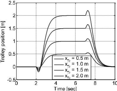
Variation of the step responses with increasing reference input magnitude is shown in Figure 22. Despite the plant nonlinearity, the step response shape does not vary visibly with the reference input magnitude.
Figure 22: Step responses with nonlinear plant model and increasing reference input magnitude.
[image:8.595.309.507.226.379.2] [image:8.595.73.273.478.630.2]Figure 23: Nominal error and worst case error envelope for +/- 10% plant parameter variations.
The peak worst case errors of 0.0166 m is acceptable. Figure 24 shows the corresponding worst case pendulum angle,
t , taken from the complete set of simulations superimposed on the pendulum angle with no parameter mismatching. It is evident that the parameter mismatching has a negligible influence on .
Figure 24: Worst case pendulum angle excursions for +/- 10% plant parameter variations.
5. Conclusions and Recommendations
The investigations show that FDC is very effective in controlling the non-minimum phase plant consisting of a trolley supporting an IP when the technique of creating a fictitious plant
output with full rank is applied. This technique may prove effective for many other non-minimum-phase plants and therefore further investigations in this direction are recommended. Regarding the IP, application of FDC using the full nonlinear plant model is recommended as this would be a useful preliminary study for control of other nonlinear non-minimum-phase plants for which the control system performance may more critically depend on use of the nonlinear model. The main problem to be solved for the IP is the formulation of the full rank fictitious output equation for the nonlinear case. Also, a preliminary study of FDC of the IP with the trolley on an inclined slope has been carried out by the authors and this indicates a steady state trolley position error. A modification of the FDC method to eliminate this error would be a worthwhile further investigation as the general method could be applied to other plants with significant constant or slowly varying external disturbances.
6. References
Dimarogonas A. D., Haddad S., Vibration for Engineers, Prentice Hall, Englewood Cliffs, NJ, 1992.
Dodds S. J., "Settling Time Formulae for the Design of Control Systems with Linear Closed Loop Dynamics, Proceedings of AC&T, University of East London, 2008.
Franklin G. F., Powell D. P. Emami-Naeini
A., Feedback Control of Dynamic Systems
(Fourth Edition), Prentice Hall, Upper Saddle River, NJ, 2002.
[image:9.595.76.273.441.595.2]Vittek J., Dodds, S. J., Forced Dynamic Control of Electric Drives, Zilina University Press, Slovakia, 2003.
Woods R. L., Lawrence, K. L., Modeling
and Simulation of Dynamic Systems,
Prentice Hall, Englewood Cliffs, NJ, 1997.
7. Appendix
Plant model without algebraic loop
Using Masons rule on Figure 12:
3 2 3
1 5
1 2 1 3 4 5 1 2 5
( ) ( )
T A s A
x s
F s s A A s A A A s A s A A A
0
3 2
2 1 0
5 ( )
( )
T b s A
x s
F s s a s a s a (23)
where b0 A1 1 A A A1 3 4 ,
2 1 2 1 1 3 4
a A A A A A , a1 A5 1 A A A1 3 4
and a0 A A A1 2 5 1 A A A1 3 4 .
For the output :
1 4
1 3 4
3 2
2 1 0
1
A A s
s A A A
F s s a s a s a
1
3 2
2 1 0
s b s
F s s a s a s a (24)
where: b1 A A1 4 1 A A A1 3 4 . Figure A1 shows the corresponding Simulink block diagram which is the state variable block diagram in the control canonical form realising transfer functions (23) and (24).
X
4 XT_dot
3 XT
2 theta_dot
1 theta 1 s
1 s 1 s 1 s
b0
b1
b1 A5
a0 a1 a2 1
F