Hydrological model calibration for derived flood frequency analysis using stochastic rainfall and probability distributions of peak flows

(1)

Hydrol. Earth Syst. Sci., 18, 353–365, 2014 www.hydrol-earth-syst-sci.net/18/353/2014/ doi:10.5194/hess-18-353-2014

Hydrology and

Earth System

Sciences

Open Access

Hydrological model calibration for derived flood frequency analysis

using stochastic rainfall and probability distributions of peak flows

U. Haberlandt and I. Radtke

Institute of Water Resources Management, Hydrology and Agricultural Hydraulic Engineering, Leibniz University of Hannover, Hannover, Germany

Correspondence to: U. Haberlandt ([email protected])

Received: 21 July 2013 – Published in Hydrol. Earth Syst. Sci. Discuss.: 14 August 2013 Revised: 20 December 2013 – Accepted: 23 December 2013 – Published: 30 January 2014

Abstract. Derived flood frequency analysis allows the

es-timation of design floods with hydrological modeling for poorly observed basins considering change and taking into account flood protection measures. There are several possi-ble choices regarding precipitation input, discharge output and consequently the calibration of the model. The objec-tive of this study is to compare different calibration strate-gies for a hydrological model considering various types of rainfall input and runoff output data sets and to propose the most suitable approach. Event based and continuous, ob-served hourly rainfall data as well as disaggregated daily rainfall and stochastically generated hourly rainfall data are used as input for the model. As output, short hourly and longer daily continuous flow time series as well as proba-bility distributions of annual maximum peak flow series are employed. The performance of the strategies is evaluated us-ing the obtained different model parameter sets for continu-ous simulation of discharge in an independent validation pe-riod and by comparing the model derived flood frequency distributions with the observed one. The investigations are carried out for three mesoscale catchments in northern Ger-many with the hydrological model HEC-HMS (Hydrologic Engineering Center’s Hydrologic Modeling System). The re-sults show that (I) the same type of precipitation input data should be used for calibration and application of the hydro-logical model, (II) a model calibrated using a small sample of extreme values works quite well for the simulation of con-tinuous time series with moderate length but not vice versa, and (III) the best performance with small uncertainty is ob-tained when stochastic precipitation data and the observed probability distribution of peak flows are used for model cal-ibration. This outcome suggests to calibrate a hydrological

model directly on probability distributions of observed peak flows using stochastic rainfall as input if its purpose is the application for derived flood frequency analysis.

1 Introduction

For reliable flood risk assessment and the development of ef-fective flood protection measures a good knowledge of flood frequencies at different points in a catchment is required. The classical approach to obtain design flows is to carry out local or regional flood frequency analysis using long records of ob-served peak discharge data (e.g., Hosking and Wallis, 1997). An alternative is to apply derived flood frequency analysis, where design floods are estimated based on simulation re-sults from a hydrological model, which is driven by observed or synthetic rainfall data. This approach is indispensable if no historical flood peak records are available for statistical anal-ysis or regionalization. Nevertheless, even if historical flood observations exist, derived flood frequency analysis provides several advantages:

– first, when using hydrological modeling for design it

is possible to consider planned alterations in land use and management, future changes in climate or the in-troduction of new flood protection measures, whose effect is not contained in observed historical flood records;

– second, hydrological modeling allows one to obtain

(2)

354 U. Haberlandt and I. Radtke: Hydrological model calibration for derived flood frequency analysis

– third, the estimation of design flows can be carried out

for completely ungauged basins if the parameters of the hydrological model are regionalized and the rain-fall model can be applied for unobserved regions. Both event based or continuous hydrological modeling is possible. A disadvantage of the event based simulation is the required assumption about equal return periods for the de-sign storm and the resulting dede-sign flood. This is usually not given, considering the required simplifying assumption about initial soil moisture conditions in the catchment, the shape and the critical duration of the design storm (Viglione and Blöschl, 2009; Verhoest et al., 2010; Grimaldi et al., 2012a). Using continuous rainfall–runoff simulation this problem can be avoided and the design flood is derived by flood frequency analysis of long series of simulated flows. However, such kinds of hydrological modeling require long continuous rain-fall series with high temporal and sufficient spatial resolu-tion. Especially for flood modeling in smaller catchments, subdaily time steps are required for simulation. Given the restricted availability of those observed data, synthetic pre-cipitation has recently been used more often for this purpose (Cameron et al., 1999; Blazkova and Beven, 2004; Aronica and Candela, 2007; Moretti and Montanari, 2008; Haberlandt et al., 2008; Boughton and Droop, 2003; Grimaldi et al., 2012b; Viglione et al., 2012).

One challenge using this approach is the optimal calibra-tion of the hydrological model considering the different na-ture of observed and synthetic precipitation data. Often, the former is used for calibration and the latter for application and design flood estimation. This procedure neglects the de-pendence of the model parameterization on the input data. For instance, Bárdossy and Das (2008) show that using dif-ferent rain gauge networks for calibration and validation of a conceptual hydrologic model leads to significantly poorer performance compared to the case when unique networks are employed. Similar problems will occur if precipitation data from different sources are used for calibration and valida-tion, such as rainfall information from point observations and weather radar (Heistermann and Kneis, 2011). In addition, if a hydrological model is calibrated using observed precipita-tion and runoff time series of high temporal resoluprecipita-tion, e.g., hourly data, which are often available only for very short time periods, the outcome might not be optimal for the sim-ulation of floods with large return periods of 50, 100 or more years.

Alternatives to using only continuous hydrographs for model calibration are the utilization of statistical flow data such as flow duration curves (Westerberg et al., 2011) or flow information in the spectral domain (Schaefli and Zehe, 2009). When flood frequency estimation is the main goal, special consideration should be given to the annual or partial peak flow series in addition to the hydrographs in the calibration process (Cameron et al., 1999; Lamb, 1999). The direct use of probability distributions of peak flow for model calibration

is apparent. However, this idea has hardly been explored in research so far.

The first objective of the paper is to compare different calibration strategies for a hydrological model operated on an hourly time step that is to be applied for derived flood frequency analysis. Event based and continuous, observed hourly rainfall data as well as disaggregated daily rainfall and stochastically generated hourly rainfall data are used as input for the model. As output, short hourly and longer daily con-tinuous flow time series as well as probability distributions of annual maximum peak flow series are employed. Second, it is hypothesized that calibrating the hydrological model di-rectly on the observed flood frequency distributions would provide the best results. This approach would have two ad-vantages: statistical peak flow data have usually much longer records of registration than continuous high resolution flow data and they permit the direct use of stochastic rainfall data for calibration of the hydrological model.

The paper is organized as follows. In Sect. 2 the methodol-ogy is presented including the precipitation models, the hy-drological model and the calibration strategies. The data and study region are described in Sect. 3. In Sect. 4 the results of the different calibration strategies for the hydrological model are discussed. Finally, Sect. 5 gives a summary of the find-ings and conclusions.

2 Methods

2.1 Precipitation modeling

A stochastic space–time precipitation model, a statistic rain-fall disaggregation model and a classical statistical design storm approach are employed here to provide precipita-tion data as input for rainfall–runoff modeling. These three rainfall generating methods are briefly introduced in the following.

2.1.1 Stochastic precipitation model

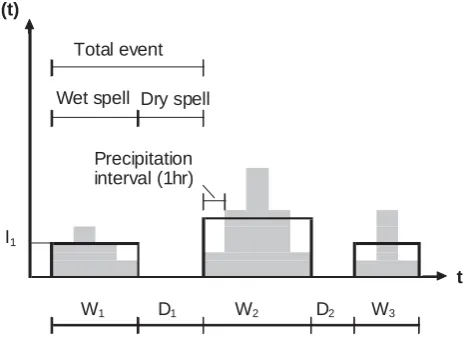
A hybrid stochastic space–time precipitation model, consist-ing of two components is used for the generation of continu-ous hourly rainfall (Haberlandt et al., 2008). The first compo-nent represents a classical alternating renewal approach for the simulation of independent precipitation event series for several locations in the domain (Fig. 1). Wet spell duration (W )and dry spell duration (D)are modeled by general ex-treme value and Weibull distributions, respectively. The wet spell intensity (I )is modeled using a Kappa distribution. The dependence between wet spell intensity and duration is de-scribed by a 2-D Frank copula (De Michele and Salvadori, 2003). For disaggregation of the wet spells into hourly inten-sities a double exponential function with random peak time is used.

(3)

U. Haberlandt and I. Radtke: Hydrological model calibration for derived flood frequency analysis 355

t Total event

Precipitation interval (1hr)

I1

Wet spell

D1

I(t)

W1 W2 D2 W3

[image:3.595.52.284.63.232.2]

Dry spell

Fig. 1. Scheme of precipitation event time series (after Haberlandt

et al., 2008).

time series (Bárdossy, 1998) with the objective to reproduce the spatial dependence structure. The objective function in-cludes three bivariate criteria: (a) the probability of rainfall occurrence, (b) Pearson’s correlation coefficient, and (c) the expected rainfall amount conditioned on rainfall occurrence at a neighboring station. The hybrid precipitation model has 11 parameters in total, which are estimated for summer (May–October) and winter seasons (November–April) sepa-rately (Haberlandt et al., 2008).

2.1.2 Rainfall disaggregation model

Often the network density and record length of daily pre-cipitation data is much better than for hourly data. So, one interesting alternative to stochastic synthesis of rainfall is the disaggregation of observed daily data into smaller time steps. For the disaggregation of daily rainfall a multiplica-tive random cascade model with exact mass conservation is used here (Güntner et al., 2001), which is a refinement of the model proposed by Olsson (1998).

The model divides the observed 24 h precipitation subse-quently into two equal sized non-overlapping boxes, having one of the three possible states with certain transition prob-abilitiesP: wet/wet withP (x/1–x), wet/dry withP(1/0) or dry/wet withP(0/1). Figure 2 shows a scheme of this ap-proach. Here, the divisions are carried out from level zero (24 h) up to level five (45 min). Hourly rainfall is finally es-timated by dividing the 45 min rainfall boxes into three uni-form 15 min blocks and reaggregating four blocks each from the time series back to 60 min. The parameters for the model are each estimated from the nearest hourly neighbor station and running the model backwards. This model does not dis-tinguish between seasons, so only one set of parameters is estimated for each station, which is then assumed valid for the whole year.

100 24 h

Level 0 45 55 1-x x 12 h 1 20

25 20 35 6 h

1-x x 1-x x 2 5 15

25 20 35

0 1 1

0 1 0

3 h 1-x x 3 5 5 10

25 20 35

1 0 1

0 1 0 1 0 1.5 h 1-x x 4 100

100 24 h

Level 0 45 55 1-x x 1-x x 12 h 1 20

25 20 35 6 h

1-x x 1-x x 1-x x 1-x x 2 5 15

25 20 35

0 1 0 1 1

0 1

0 11 00

3 h 1-x x 1-x x 3 5 5 10

25 20 35

1 0 1

0 1 0 1

0

1.5 h

1-x x

4 25 10 5 5 20 35

1 0 1 0 1

0 1 0 11 00 1 0 1 0 1.5 h 1-x x 1-x x 4

Fig. 2. Scheme of a multiplicative random cascade model (modified

after Olsson, 1998).

The main problem with this disaggregation approach is the conservation of the space–time structure of precipitation. In the presented study a simple method is used to create spatial dependence. First, daily precipitation time series were disag-gregated using the random cascade. In the next step for every day the station with the highest daily precipitation amount is selected. Their diurnal variation, obtained from disaggrega-tion, is then applied on all other stations in the catchment. It is accepted here that this results in spatially more homoge-neous than natural precipitation, which may lead to an over-estimation of the observed floods.

2.1.3 Statistical design storm approach

The classical approach for the estimation of design floods based on rainfall–runoff modeling uses statistical storms derived from rainfall intensity-duration-frequency (IDF) curves. In Germany a regionalized version of IDF curves called KOSTRA is available (Bartels et al., 2005). KOSTRA provides statistical design storms on a raster for the whole of Germany with cell sizes of 8.45 km×8.45 km for durations between 5 min and 72 h and for return periods from 0.5 yr up to 100 yr.

For rainfall–runoff modeling areal precipitation data in-stead of point values are necessary. Areal reduction factors are a common method to adjust point extreme rainfall to rainfall for larger areas. Here an areal reduction method es-pecially derived for German conditions depending on catch-ment size and rainfall duration is applied (Verworn, 2008).

[image:3.595.312.547.69.184.2]

(4)

30

Figure 3. HEC-HMS model (adapted from Feldmann, 2000)

infiltration

runoff concentration

baseflow canopy

interception

surface

depression Clark

unit hydrograph surface runoff

linear reservoir 2 linear reservoir 1

runoff formation

interflow

baseflow soil storage precipitation evapotranspiration

surface runoff

upper GW-storage

lower GW-storage upper zone

storage tension zone

storage percolation

percolation

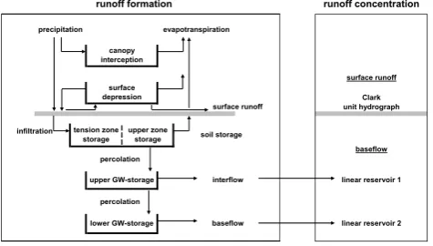
Fig. 3. HEC-HMS model (adapted from Feldmann, 2000).

2.2 Rainfall–runoff modeling

In this section, first the applied rainfall–runoff model is briefly presented and then the different strategies for model calibration and application based on the diverse input and output data sets are discussed.

2.2.1 Rainfall–runoff model

For rainfall–runoff modeling the conceptual semidistributed model HEC-HMS (Hydrologic Engineering Center’s Hydro-logic Modeling System; Feldmann, 2000) has been chosen, which comprises typical concepts used for flood simulations and allows sufficient fast computations with larger data sets. HEC-HMS offers different methods for the simulation of the processes of runoff formation, runoff concentration and flood routing. Additionally, several possibilities exist for the calcu-lation of areal precipitation and potential evaporation. Here, the model is operated continuously at an hourly time step with the structure depicted in Fig. 3.

The soil moisture accounting (SMA) algorithm is used for runoff generation, the Clark unit hydrograph for the trans-formation of direct runoff, two linear reservoirs to consider interflow and base flow transformation, and simple river routing is employed where the flows are only lagged in time. Snowmelt is calculated externally using the tempera-ture index method. Potential evaporation is also computed externally using the method proposed by Turc–Wendling (Wendling et al., 1991), based on observed temperature and global radiation data; and is corrected according to the dif-ferent vegetation types in the subcatchments. Then the mean monthly values over the simulation period are used as input for HEC-HMS scaled according to the simulation time step. This simple approach can be justified here by the compari-son character of the model application. Actual evapotranspi-ration is simulated in HEC-HMS depending on the potential evapotranspiration and the water availability from canopy, surface and soil storages. To account for spatial heterogene-ity of climate data and basin characteristics the catchments are spatially divided into several subcatchments and river

[image:4.595.307.544.62.154.2]

31 Figure 4. Calibration strategies leading to the parameter sets A to E; the temporal resolution of the data is given in brackets

Observed precipitation data

[1h]

Disaggregated daily precipitation data

[1h]

Stochastic precipitation data

[1h]

Single flood events

[1h]

Continuous hydrograph [1h]

Continuous hydrograph [1d]

Flood frequency distribution

[-]

A B C D E

Precipitation input

Parameter sets

Discharge observed

Observed precipitation data

[1h]

Single flood events

[1h]

Continuous hydrograph [1d]

Flood frequency distribution

[-]

A B C D E

Precipitation input

Parameter sets

Discharge observed

Fig. 4. Calibration strategies leading to the parameter sets A–E; the

temporal resolution of the data is given in brackets.

reaches. The input data precipitation and potential evapora-tion are estimated as areal averages for the subcatchments using Thiessen interpolation from station data.

2.2.2 Strategies for model calibration

The calibration of HEC-HMS is done automatically in lumped mode for the catchment under investigation using the PEST (Parameter Estimation) algorithm (Doherty, 2005). Five parameters are selected for calibration comprising the storage coefficients for the upper and lower groundwater reservoirs in the runoff formation module, the storage coef-ficients for the two linear reservoirs describing runoff con-centration for interflow and baseflow, respectively, and the storage coefficient for the Clark unit hydrograph referring to surface runoff concentration (see Fig. 3). These are all conceptual parameters, which are difficult to estimate from physical catchment properties, and they have been tested to be sensitive for calibration.

As objective functions, the squared sum of deviations be-tween observed and simulated flows is used. For performance assessment the Nash–Sutcliffe criterion and the bias are em-ployed. Figure 4 gives an overview of the calibration strate-gies used in this investigation. Five calibration stratestrate-gies are shown, which can be distinguished by their different input and output data. Each calibration strategy leads to a unique parameter set, indicated by the letters A through E.

Parameter set A is obtained with event based calibration using a number of observed rainfall–runoff events simulta-neously. Since the initial conditions are unknown, storage contents for each event are also included in the calibration. Validation for this parameter set is done using continuous modeling based on data sets from strategy B.

Parameter set B is estimated by calibration of the model using continuous hourly observed precipitation and dis-charge data for the short observation period of some years. Validation of the resulting parameter set is done by split sam-pling for another couple of years.

[image:4.595.49.287.64.199.2]

(5)

So, for direct comparison of simulated and observed flows only daily data can be used. Since hourly precipitation results from a statistical disaggregation model, 10 realizations are generated and the median of the 10 simulated flow time se-ries aggregated to daily values is used for calibration against observations. This is a compromise to consider the stochastic character of the precipitation input using one unique param-eter set, which however may lead to a certain loss of variance in flow simulations. Validation of parameter set C is done us-ing split samplus-ing on the longer daily flow time series and using the shorter hourly hydrographs from strategy B. An advantage of this calibration strategy using daily data is the availability of longer observation records comprising often more than 30 yr and denser precipitation networks.

For the calibration of the model to estimate parameter set D, disaggregated precipitation and the observed flood fre-quency distributions of the same time period are utilized. Again, 10 realizations of disaggregated precipitation data are used for hydrological simulations. Independent flood events are selected from the continuously simulated flows using a minimum of 10 d intraevent time considering the catchment sizes in this study (see section 3). Annual series (January– December), summer series (May–October) and winter series (November–April) of peak flows are compiled from observed and simulated data. To mitigate sampling errors, a theoretic probability distribution is fitted to the series of observed and simulated peak flows. Here the generalized extreme value distribution (GEV) with parameter estimation based on L moments is chosen (Hosking and Wallis, 1997). For calibra-tion a number of recurrence intervals are selected for which flow quantiles are estimated from the GEV distributions. Theoretical quantiles obtained from the distributions fitted to observed peak flow series are considered as “observations”. The medians of the theoretical quantiles from the distribu-tions fitted to the 10 simulated series are considered as “simu-lations”. The pairs of recurrence intervals and quantiles build the supporting points in the objective function. For calibra-tion the distribucalibra-tions of annual, winter and summer seasons are considered simultaneously and the supporting points are weighted proportionally to their return periods. Validation of parameter set D is done using 10 different precipitation real-izations and by evaluations of continuous simulation consid-ering the observed periods from strategy B. The advantage of this strategy is the direct use of hourly disaggregated rainfall and of observed flood quantiles in the calibration process.

The last calibration strategy to estimate parameter set E uses continuous stochastic rainfall and observed flood fre-quency distributions. The procedure of parameter estimation is basically the same as for parameter set D. The main dif-ference is the missing time redif-ference of the stochastic rain-fall and the possibility to generate time series of any length. Therefore all observed annual and seasonal maximum floods can be used for fitting the “observed” GEV. Using very long time series may reduce the sampling error but would re-quire more computation time. So, considering that the full

[image:5.595.308.548.62.157.2]

32 Figure 5. Strategies for the estimation of design floods; the temporal resolution of the data is given in brackets

A

B

C

D E

KOSTRA Single storm

[1h]

[1h] Precipitation

input

Parameter sets

Discharge output

Single flood event

[1h]

Design flood Direct estimation Statistical analysis of simulated floods

B B

A

B

C

D E

KOSTRA Single storm

[1h]

[1h] Precipitation

input

Parameter sets

Discharge output

Single flood event

[1h]

Design flood Direct estimation Statistical analysis of simulated floods

B B

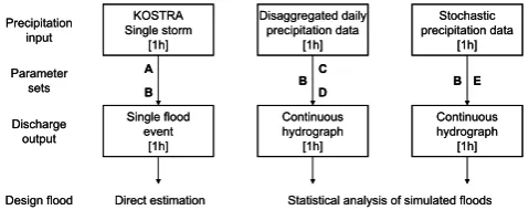
Fig. 5. Strategies for the estimation of design floods; the temporal

resolution of the data is given in brackets.

time series are employed for the automatic calibration pro-cess with many iterations the length has been restricted here to 100 yr. Again, 10 realizations are generated for model cal-ibration in order to consider the uncertainty of the precipita-tion process. The validaprecipita-tion of parameter set E is done us-ing another 10 precipitation realizations and the continuous hourly data from strategy B.

2.2.3 Strategies for estimation of design floods

Considering the five estimated parameter sets A–E and the different precipitation forcings, several alternatives for the application of the hydrological model to estimate design flows are possible. Figure 5 shows the strategies that are used and compared here regarding estimation performance and uncertainty.

For the event based rainfall–runoff modeling the statisti-cal KOSTRA precipitation data are applied (see Sect. 2.1.3) assuming equal return periods for rainfall and resulting peak flow. Considering catchment size, the model is run for differ-ent storm durations around the time of concdiffer-entration, while only that hydrograph is kept, which produces the largest peak. Regarding initial conditions the model starts up with mean storage contents for soil and groundwater reservoirs obtained from the calibration over all events and a base flow that is equal to the long-term mean discharge. Taking aver-age antecedent conditions as initial values for design is of-ten the usual choice and works well in practice (Pilgrim and Cordery, 1993; Viglione et al., 2009). Uncertainty in initial conditions is considered by varying the storage contents by plus/minus 10 and 20 % around the mean. Uncertainty in pre-cipitation is considered here taking into account an error of up to plus/minus 20 % according to Bartels et al. (2005) for the KOSTRA data. So, all together 15 model runs are used for the estimation of the design flow and its uncertainty at each return period. The whole procedure is applied for the two parameter sets A and B.

(6)

[image:6.595.54.286.64.212.2]

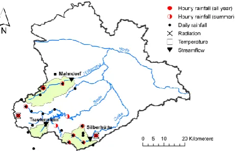
Fig. 6. Study area with the three selected catchments, precipitation

stations, climate stations and stream flow gauges.

and validation together are used to consider uncertainty. Rainfall–runoff modeling with disaggregated precipitation data is done using the parameter sets B, C and D. If the stochastic precipitation data are used as model input, param-eter sets B and E are employed.

3 Study area and data

The investigations are carried out for three mesoscale catch-ments within the Bode River basin in northern Germany: the Silberhütte catchment with a drainage area of 105 km2, the Mahndorf catchment with an area of 168 km2and the Traut-enstein catchment with an area of 39.1 km2(see Fig. 6).

The Bode region has elevations between 1140 m a.s.l. at the top of the Brocken Mountain and about 80 m a.s.l. at the lowest point where the Bode River flows into the Saale River. Mean annual rainfall varies between 1700 and 500 mm yr−1. Floods are generated either by frontal rainfall, frontal rainfall on snow smelt or convective storms.

Observed precipitation data at an hourly time step are available for about 14 yr of the time period from 1993 to 2006 and at a daily time step in the period between 1968 and 2005. Most of the hourly stations are only available for the summer season. The climate data temperature and radiation are available for the same two temporal resolutions and time periods at three and two locations, respectively. Observed discharge is available as daily flows and monthly peak flow series within the period from 1948 to 2005 with lengths be-tween 33 and 56 yr for the three streamflow gauges. In addi-tion, hourly flow time series are available for the period from 1998 to 2004. Table 1 lists the volume of the data, which can be utilized for calibration, validation and application for each calibration strategy.

The strategies A and B, which use hourly data, have to rely on only seven years of observations for both calibra-tion and validacalibra-tion. The network density is increased here by employing daily rainfall from the non-recording network

disaggregated by rescaling the hourly rainfall profile from the nearest recording station. An observation period of 33–35 yr in total is available when daily flow and precipitation data are employed (strategies C and D). If stochastic rainfall is used in strategy E the maximum observed record length of about 50 yr for peak flow series can be utilized. Also in this case the network density is increased to the same degree as in strat-egy A and B by using rescaled hourly stochastic rainfall at the locations of daily stations from the nearest recording sta-tion. Hydrologic modeling is done in strategy E with 100 yr of stochastic rainfall even if the reference time series for cal-ibration and application are shorter. This requires providing climate data for 100 yr at an hourly time step. For calculation of potential evapotranspiration the observed mean monthly values are used (see Sect. 2.2.1); for snowmelt simulations observed time series of temperature over 25 yr are simply re-sampled four times to provide the input. Strategies D and E use for calibration and validation the same observed peak flows but 10 different realizations of stochastic rainfall. In ad-dition, validation is carried out for all strategies on observed hourly flow time series.

For the application and uncertainty assessment of strate-gies D and E all 20 realizations are used. This is not a very large sample size, but the number of realizations had to be restricted considering hourly simulations and the demanding recalibration requirements for each strategy. Since this study focusses on relative comparisons and not on absolute design values this is regarded here as acceptable.

4 Analyses and results

In this section first the performances of the stochastic rainfall model and the statistic disaggregation approach are briefly presented. Then the results of calibration and validation of the hydrological model using the different data and param-eter sets are discussed. The hydrological model is applied for the estimation of flood frequency distributions and de-sign floods to compare the performance and uncertainty of the different alternatives.

4.1 Performance of precipitation modeling

For validation of the stochastic precipitation model 10 real-izations of hourly rainfall, each 100 yr in length are generated for all hourly stations. For validation of the disaggregation model also 10 realizations of hourly rainfall are disaggre-gated using aggredisaggre-gated daily rainfall from the same hourly stations.

(7)

[image:7.595.98.499.94.172.2]

Table 1. Average data volume available for calibration, validation and application for hydrological modeling depending on calibration

strategy (see Fig. 4).

Calibration strategy Data for calibration Data for validation Application

A 13 events No separate events Statistical rainfall

B 4 yr 3 yr see A, D or E

C 15 yr 20 yr see A, D, or E

D 35 yr (10 realizations) 35 yr (10 realizations) 35 yr (20 realizations) E 50/100 yr∗(10 realizations) 50/100 yr∗(10 realizations) 100 yr (20 realizations)

* About 50 yr of discharge data and 10 realizations of 100 yr of precipitation data

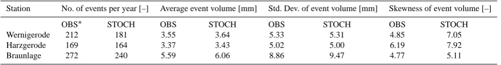
Table 2. Event characteristics for three selected rainfall stations (see Fig. 6) from 14 yr observed rainfall (OBS) and 10×100 yr stochastic generated rainfall (STOCH); OBS statistics estimated from data with missing values as gaps.

Station No. of events per year [–] Average event volume [mm] Std. Dev. of event volume [mm] Skewness of event volume [–] OBS∗ STOCH OBS STOCH OBS STOCH OBS STOCH Wernigerode 212 181 3.55 3.64 5.33 5.31 4.85 7.05 Harzgerode 169 164 3.37 3.43 5.02 5.00 6.19 7.92 Braunlage 272 240 5.59 6.06 8.86 9.47 4.77 5.11

* Adjusted according to relative gap contribution to observation period.

models. For stochastic rainfall good agreement between sim-ulated and observed statistics is reached. Some underestima-tion of the number of events and a small overestimaunderestima-tion of the event volume occurs. While the standard deviation is also reproduced quite well, the skewness is reproduced poorly.

For disaggregated rainfall sufficient agreement between observed and simulated statistics is found. The number of events is overestimated and the event volume is underesti-mated. Higher order moments are only roughly reproduced. Comparing the results between both models shows that the pure stochastic rainfall model has a better performance as the statistics disaggregation approach except for the simula-tion of the skewness. Note that the observed statistics dif-fer between stochastic modeling and the disaggregation ap-proach because for disaggregation the gaps in the data had to be filled prior to the application.

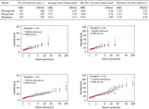
In addition, a frequency analysis is carried out on the an-nual maximum precipitation series for observed and simu-lated rainfall using different durations. Selected results are presented in Fig. 7. For the disaggregation approach rainfall can only be provided for the observed period, which is very short here for precipitation validation. For the stochastic pre-cipitation model rainfall can be generated for longer periods but can only be compared to the short observation statistic. It can be seen that the observed values are plotted mostly within the range of the simulated realizations. For disaggre-gated rainfall the range among the 10 realizations is some-what larger as for the pure synthetic rainfall realizations. For the stochastic model a slight overestimation of the observed extreme values occurs for larger return periods and durations. Considering the short observation periods it is difficult to val-idate the models regarding the synthesis of more extreme

rainfall intensities. This will be further addressed with hy-drological modeling.

More information about application and validation of the precipitation models, especially regarding the conservation of spatial consistence of rainfall, is provided in Haberlandt et al. (2008) and about the disaggregation approach in Ebner von Eschenbach et al. (2008).

4.2 Performance of the hydrological model and

estimation of design floods

[image:7.595.55.545.230.294.2]

(8)

Table 3. Event characteristics for three selected rainfall stations (see Fig. 6) from 14 yr OBS and 10×14 yr DISAG rainfall; OBS statistics estimated from data with missing values replaced by data from neighbor stations.

Station No. of events per year [–] Average event volume [mm] Std. Dev. of event volume [mm] Skewness of event volume [–] OBS DISAG OBS DISAG OBS DISAG OBS DISAG Wernigerode 165 206 3.77 3.07 6.04 4.44 7.29 7.51 Harzgerode 163 202 3.37 2.72 5.04 3.79 6.14 7.07 Braunlage 252 297 5.63 4.77 8.92 6.85 4.79 4.29

34 Figure 7

. Empirical probability distributions of annual maximum precipitation from observed

(OBS), disaggregated (DISAG, top row) and stochastically generated rainfall (STOCH,

bottom row) for the station Harzgerode for 1 hour and 4 hour durations

1 2 5 10 20 50 100

0 20 40 60 80

Return period [yr]

Rainf

all [mm]

Duration = 1 hr

DISAG (10x14 yr) OBS (14 yr)

1 2 5 10 20 50 100

0 20 40 60 80 100 120

Return period [yr]

Rainf

all [mm]

Duration = 4 hr

DISAG (10x14 yr) OBS (14 yr)

1 2 5 10 20 50 100

0 20 40 60 80

Return period [yr]

Rainf

all [mm]

Duration = 1 hr

STOCH (10x100 yr) OBS (14 yr)

1 2 5 10 20 50 100

0 20 40 60 80 100 120

Return period [yr]

Rainf

all [mm]

Duration = 4 hr

STOCH (10x100 yr) OBS (14 yr)

Fig. 7. Empirical probability distributions of annual maximum precipitation from OBS, DISAG (top row) and STOCH rainfall (bottom row)

for the station Harzgerode for 1 and 4 h durations.

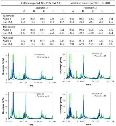
set B obtained directly using those data. Parameter sets A and C obtained from calibration on single events and daily discharge are also suitable to reproduce the hourly flow hy-drographs. Figure 8 shows the simulated hydrographs using observed precipitation for the validation period for four of the five different parameter sets. The visual assessment con-firms the findings in Table 4. The simulated hydrographs for all parameter sets are quite similar. Higher peak flows were simulated when the model is calibrated on the extreme value distributions (parameter sets D and E). This is especially true for parameter set D, which results from disaggregated rain-fall, considering the three highest peaks in the simulation pe-riod. The reason for this might be the forced, spatially con-sistent timing of rainfall peaks for all stations involved in the disaggregation approach (see Sect. 2.1.1). Based on the above validation all parameter sets are considered generally suitable for hydrological modeling.

After this initial validation of the hydrological model, de-sign floods are estimated using all parameter sets succes-sively for the three catchments. First, the results are dis-cussed more in detail for the Silberhütte catchment. Then, a comparison of the 50 yr design flood estimation for all catch-ments and parameter sets is presented.

[image:8.595.56.541.92.445.2]

(9)

[image:9.595.92.503.80.525.2]

Table 4. Validation of the calibrated parameter sets using the Nash–Sutcliffe criterion (NSC) and the bias.

Calibration period: Nov 1997–Oct 2001 Validation period: Nov 2001–Oct 2004

Parameter set Parameter set

A B C D E A B C D E

Silberhütte

NSC [-] 0.86 0.87 0.86 0.85 0.83 0.82 0.83 0.82 0.86 0.81

Bias [%] 13.4 13.5 13.4 13.8 13.5 20.4 20.2 20.4 20.0 20.2

Trautenstein

NSC [-] 0.84 0.86 0.84 0.85 0.81 0.82 0.82 0.78 0.82 0.79

Bias [%] −1.99 −2.28 −1.71 −2.26 −2.39 −22.7 −22.3 −23.0 −22.4 −22.1

Mahndorf

NSC [-] 0.52 0.72 0.77 0.46 0.44 0.63 0.78 0.67 0.53 0.52

Bias [%] −14.6 −16.6 −18.5 −16.1 −14.7 −7.04 −6.90 −5.45 −7.19 −7.20

Figure 8:

Simulated hydrographs using four different parameter sets A, B, D and E based on

observed hourly precipitation for the validation period from November 2001 to October 2004

0 5 10 15 20

01.11.01 01.11.02 01.11.03 01.11.04

Time

Disc

harge [

m

³/

s]

Observed Parameter set A

0 5 10 15 20

01.11.01 01.11.02 01.11.03 01.11.04

Time

Disc

harge [

m

³/

s]

Observed Parameter set B

0 5 10 15 20

01.11.01 01.11.02 01.11.03 01.11.04

Time

Disc

harge [

m

³/

s]

Observed Parameter set D

0 5 10 15 20

01.11.01 01.11.02 01.11.03 01.11.04

Time

Disc

harge [

m

³/

s]

Observed Parameter set E

Fig. 8. Simulated hydrographs using four different parameter sets A, B, D and E based on observed hourly precipitation for the validation

period from November 2001 to October 2004.

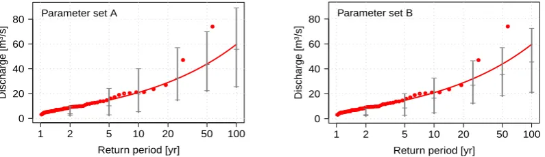
25 and 100 yr. The bars enclose the 90 %-confidence inter-val, which represents the 5 and 95 % empirical quantiles es-timated from the 15 model runs each (i.e., the single highest and lowest value is excluded; see also Sect. 2). From com-paring observations, i.e., the fitted GEV to observed peak flows, with the simulated range of design flows, a good agree-ment can be seen. However the extent of the bars is wide, indicating quite a bit of uncertainty. The range of simula-tions from parameter set A covers better the observasimula-tions but is larger than for parameter set B. Also, with parameter set B smaller design floods are estimated. A possible reason

for that might be the calibration of parameter set B for con-tinuous flow series trying to simulate the total hydrograph reasonably well, not only the flood events as for parameter set A. The main results are consistent also for the other two catchments.

The results from design flood estimation with continuous rainfall–runoff modeling and disaggregated precipitation for the Silberhütte catchment are shown in Fig. 10. The hydro-logical model is run continuously over a period of 36 yr, where daily precipitation for disaggregation was available. GEV distributions are fitted to the observed and simulated

(10)

36 Figure 9. Range and median of simulated design flows based on 15 model runs using KOSTRA

rainfall data representing the 90%-confidence interval against observed peak flows for the

Silberhütte catchment; left: parameter set A, right: parameter set B

1 2 5 10 20 50 100

0 20 40 60 80

Return period [yr]

Discharge [m³/s]

− −

− − −

− −

−

− −

Parameter set A

1 2 5 10 20 50 100

0 20 40 60 80

Return period [yr]

Discharge [m³/s]

− −

− − −

− −

−

− −

[image:10.595.101.499.63.178.2]

Parameter set B

Fig. 9. Range and median of simulated design flows based on 15 model runs using KOSTRA rainfall data representing the 90 %-confidence

interval against observed peak flows for the Silberhütte catchment; left: parameter set A, right: parameter set B.

annual maximum peak flows for this period and extrapolated here only up to the 50 yr recurrence interval considering the restricted data period. The simulated range of peak flows en-closes the 90 %-confidence limits, which represents the 5 and 95 % empirical quantiles estimated for selected return peri-ods from the 20 realizations (i.e., the single highest and low-est value is excluded). Similar ranges of simulated flows can be seen for parameter sets B and C. However, smaller peak flows are obtained for parameter set C, where the model has been calibrated on daily hydrographs, which is a reasonable outcome. The uncertainty band that results from using pa-rameter set D is the smallest, but the range does not cover the observations completely and the slope is somewhat different from the observed distribution. This outcome might be an ar-tifact of the calibration. Again, similar results were obtained for the other two catchments.

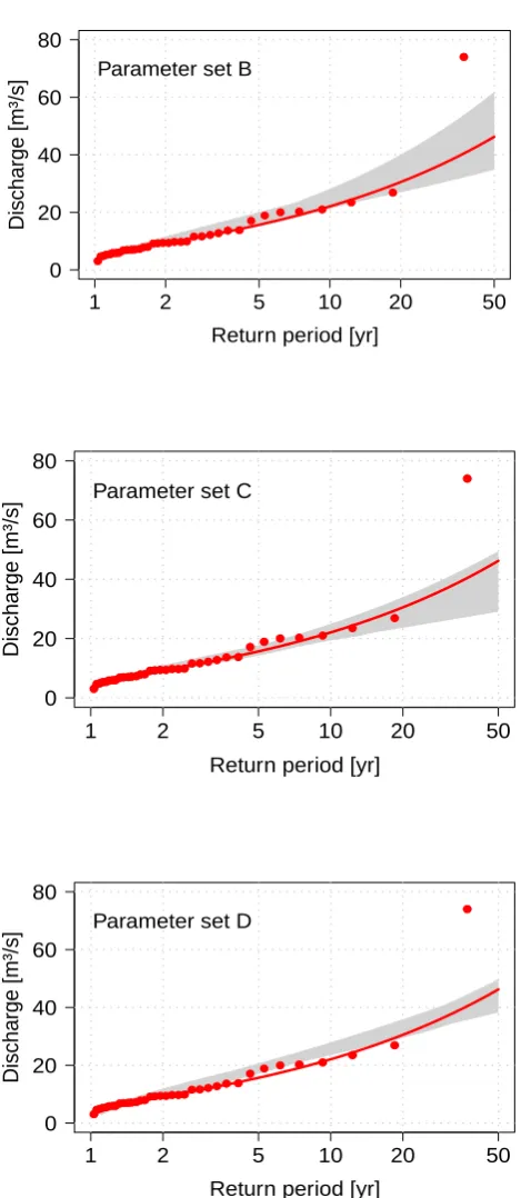
The results from using stochastic precipitation to estimate the design floods are shown in Fig. 11 for the Silberhütte catchment. The hydrological model is run continuously over a period of 100 yr for 20 realizations of stochastic rainfall. GEV distributions are fitted to observed peak flows for the total observation period of 56 yr and to simulated peak flows for each realization of 100 yr length. The 90 %-confidence limits are set up again using 5 and 95 % empirical quantiles for selected return periods from the total number of 20 real-izations (i.e., the single highest and lowest value is excluded). Applying the precalibrated model based on observed precip-itation with parameter set B leads to an overestimation of peak flows with a wide uncertainty range. If instead calibra-tion on the extreme value distribucalibra-tion of observed flows is carried out and parameter set E is applied the uncertainty is reduced, as seen by the smaller confidence band. In addition, the simulated peak flow distributions cover the observed one very well in this case, showing a better model performance compared to the application of parameter set B. Again, simi-lar results were obtained for the other two catchments.

Finally, to sum up the results, a comparison for the es-timation of the 50 yr flood including uncertainty bands for the different calibration strategies and all three catchments is presented in Fig. 12. In order to consider the error from

the restricted length of the observed flow records a paramet-ric bootstrap is applied to estimate the confidence intervals for the estimated 50 yr flood from observations (Davison and Hinkley, 2005). Note that the uncertainty bands of the ob-served floods differ slightly according to the different sam-ple sizes used in calibration and application as reference for the three cases: statistic design rainfall (KOSTRA) with about 50 yr, disaggregated rainfall (DISAG) with about 35 yr and stochastic rainfall (STOCH) again with about 50 yr. The classical calibration using single events with design storms (KOSTRA and parameter set A) provides good estimations for the Silberhütte and Mahndorf catchments, but an overes-timation for the Trautenstein catchment. However, the confi-dence intervals are widest for this parameter set. Using pa-rameter set B obtained from calibration with short hourly hydrographs for KOSTRA rainfall leads to less accurate esti-mations but with somewhat smaller error bands. If parameter set B is applied with disaggregated rainfall or with stochastic rainfall the estimation performance is generally poor. Param-eter set C, which was obtained by calibration on daily flow data performs not much better than parameter set B for dis-aggregated rainfall but with smaller uncertainty. The most suitable calibration strategies for the estimation of the design flood seem to be the ones that use the observed flood peak distributions together with the synthetic rainfall data for cal-ibration. These are the cases based on parameter set D with disaggregated precipitation and parameter set E with stochas-tic rainfall. It is remarkable that for all catchments the uncer-tainty bands can be reduced considerably if parameter sets D and E are applied.

5 Summary and conclusions

(11)

Figure 10

. Range of simulated design flows based on 20 model runs using 35 years of

disaggregated precipitation data representing the 90%-confidence interval against observed

peak flows for the Silberhütte catchment for different parameter sets

1 2 5 10 20 50

0 20 40 60 80

Return period [yr]

Discharge [m³/s]

Parameter set B

1 2 5 10 20 50

0 20 40 60 80

Return period [yr]

Discharge [m³/s]

Parameter set C

1 2 5 10 20 50

0 20 40 60 80

Return period [yr]

Discharge [m³/s]

[image:11.595.50.285.86.626.2]

Parameter set D

Fig. 10. Range of simulated design flows based on 20 model runs

using 35 yr of disaggregated precipitation data representing the 90 %-confidence interval against observed peak flows for the Sil-berhütte catchment for different parameter sets.

peak flow series are employed. The main results can be sum-marized as follows:

– using a different type of rainfall data for model

cali-bration and application usually leads to less accurate results for the application than compared to when the same type of data are used. These results are in line with findings of Bárdossy and Das (2008) regarding network density or of Heistermann and Kneis (2011) with respect to different rainfall data sets and spatial interpolation methods;

– the hydrological model works quite well for general

conditions, i.e., reproducing the hydrograph on the whole, when it is calibrated on extreme conditions, i.e., using the extreme value distribution of peak flows, than vice versa. This confirms that unusual events or small data sets might be sufficient for model calibra-tion (Singh and Bárdossy, 2012; Seibert and Beven, 2009);

– the best performance and a small uncertainty for

de-sign flood estimation over all catchments is obtained if stochastic precipitation data are used for calibra-tion on the observed probability distribucalibra-tion of peak flows. Similar good results can be obtained with disag-gregated daily rainfall data. However, this latter strat-egy has some limitations for the estimation of design floods with larger return periods because of the re-stricted length of the observation period;

– the classical event based design flood estimation works

surprisingly well here for two of the three catch-ments but comes along with a quite high uncertainty. Nonetheless, also in this case it is better to use the same type of precipitation data for calibration and applica-tion, i.e., the single events, compared to using continu-ous rainfall and discharge for calibration but the design storms for application.

The applicability of the calibration strategy based on prob-ability distributions of peak flow depends of course on the quality of the observed peak flow series. If these are too short larger floods may have the wrong plotting position and the calibration will overestimate the floods. Special problems could also arise from different flood generating mechanisms in a catchment, which may lead to step changes in the flood frequency curves (Rogger et al., 2012), which then needs to be considered in distribution fitting and model calibration. The uncertainty of the precipitation model parameters are not considered here and may increase the total error bands. Also, the uncertainty resulting from the hydrological model param-eter sets is not discussed here. Further analyses have shown that this error is larger than the variability that comes from the different rainfall realizations (Radtke, 2012).

One main purpose of this paper was to introduce the idea of calibrating a hydrological model based on flood

(12)

38 Figure 11

. Range of simulated design flows based on 20 model runs using 100 years of

stochastic precipitation data representing the 90%-confidence interval against observed peak

flows for the Silberhütte catchment for different parameter sets

1 2 5 10 20 50 100

0 20 40 60 80 100 120

Return period [yr]

Discharge [m³/s]

Parameter set B

1 2 5 10 20 50 100

0 20 40 60 80 100 120

Return period [yr]

Discharge [m³/s]

Parameter set E

Fig. 11. Range of simulated design flows based on 20 model runs using 100 yr of stochastic precipitation data representing the 90

%-confidence interval against observed peak flows for the Silberhütte catchment for different parameter sets.

0 20 40 60 80

Discharge [m³/s]

Silberhütte

OBS A B C D E

− −

−

− −

− − −

−

− −

−

KOSTRA DISAG STOCH

0 20 40 60 80 100 120

Discharge [m³/s]

Mahndorf

OBS A B C D E

− −

−

− −

− − −

−

− −

− ₋

− −

−

KOSTRA DISAG STOCH

0 10 20 30 40 50 60 70

Discharge [m³/s]

Trautenstein

OBS A B C D E

−

− −

−

− −

−

− −

−

− −

−

[image:12.595.101.499.62.179.2]

KOSTRA DISAG STOCH

Fig. 12. Estimated 50 yr floods with 90 %-confidence bands for the

three catchments and the five data sets (A–E) obtained from the dif-ferent calibration strategies using KOSTRA, DISAG and STOCH precipitation in comparison to flood estimation based on observed annual maximum flows (OBS).

frequency distributions using stochastic rainfall and to eval-uate it against classical strategies in an empirical case study. The results have shown the suitability of this approach. How-ever, more research is required to further test this model cali-bration strategy on stochastic input and output data involv-ing diverse catchments and different hydrological models. Generally, this approach may also be suitable in climate im-pact studies where hydrological models could be calibrated directly using the simulated precipitation from regional cli-mate models against observed flow statistics. Such an appli-cation of the model calibration strategy is currently under investigation.

Acknowledgements. Research leading to this paper was partly

supported by the German Federal Ministry of Education and Research (BMBF) in the framework of the RIMAX program (FKZ: 0330684). The authors thank the water authorities from Saxony-Anhalt (LHW) and the German Weather Service (DWD) for providing the hydrological and meteorological data, respec-tively. We also thank the two anonymous reviewers and the editor for their valuable comments, which helped to improve the paper.

Edited by: J. Freer

References

Aronica, G. T. and Candela, A.: Derivation of flood frequency curves in poorly gauged Mediterranean catchments using a sim-ple stochastic hydrological rainfall-runoff model, J. Hydrol., 347, 132–142, 2007.

Bárdossy, A.: Generating precipitation time series using simulated annealing, Wat. Resour. Res., 34, 1737–1744, 1998.

Bárdossy, A. and Das, T.: Influence of rainfall observation network on model calibration and application, HESS, 12, 77–89, 2008. Bartels, H., Dietzer, B., Malitz, G., Albrecht, F. M., and

[image:12.595.50.285.238.630.2]

(13)

Blazkova, S. and Beven, K.: Flood frequency estimation by continu-ous simulation of subcatchment rainfalls and discharges with the aim of improving dam safety assessment in a large basin in the Czech Republic, J. Hydrol., 292, 153–172, 2004.

Boughton, W. and Droop, O.: Continuous simulation for design flood estimation–a review, Environ. Modell. Softw., 18, 309–318, doi:10.1016/S1364-8152(03)00004-5, 2003.

Cameron, D. S., Beven, K. J., Tawn, J., Blazkova, S., and Naden, P.: Flood frequency estimation by continuous simulation for a gauged upland catchment (with uncertainty), J. Hydrol., 219, 169–187, 1999.

Davison, A. C. and Hinkley, D. V.: Bootstrap methods and their applications, 7 Edn., Cambridge University Press, New York, 582 pp., 2005.

De Michele, C. and Salvadori, G.: A Generalized Pareto intensity-duration model of storm rainfall exploiting 2-Copulas, J. Geo-phys. Res., 108, 4067, doi:4010.1029/2002JD002534, 2003. Doherty, J.: PEST: Model Independent Parameter Estimation, 5th

Edn. of user manual, Watermark Numerical Computing, Bris-bane, Australia, 2005.

Ebner von Eschenbach, A.-D., Haberlandt, U., Buchwald, I., and Belli, A.: Ermittlung von Bemessungsabflüssen mit N-A-Modellierung und synthetischem Niederschlag, Wasser-wirtschaft, 11, 19–23, 2008.

Feldmann, A. D.: Hydrologic Modeling System HEC-HMS, Tech-nical Reference Manual, US Army Corps of Engineers, Hydro-logic Engineering Center, Davis, CA, 2000.

Grimaldi, S., Petroselli, A., and Serinaldi, F.: Design hydrograph estimation in small and ungauged watersheds: continuous sim-ulation method versus event-based approach, Hydrol. Process., 26, 3124–3134, doi:10.1002/hyp.8384, 2012a.

Grimaldi, S., Petroselli, A., and Serinaldi, F.: A continuous simulation model for design-hydrograph estimation in small and ungauged watersheds, Hydrol. Sci. J., 57, 1035–1051, doi:10.1080/02626667.2012.702214, 2012b.

Güntner, A., Olsson, J., Calver, A., and Gannon, B.: Cascade-based disaggregation of continuous rainfall time series: the influence of climate, Hydrol. Earth Syst. Sci., 5, 145–164, doi:10.5194/hess-5-145-2001, 2001.

Haberlandt, U., Ebner von Eschenbach, A.-D., and Buchwald, I.: A space-time hybrid hourly rainfall model for derived flood frequency analysis, Hydrol. Earth Syst. Sci., 12, 1353–1367, doi:10.5194/hess-12-1353-2008, 2008.

Heistermann, M. and Kneis, D.: Benchmarking quantitative precip-itation estimation by conceptual rainfall-runoff modeling, Water Resour. Res., 47, W06514, doi:10.1029/2010wr009153, 2011. Hosking, J. R. M. and Wallis, J. R.: Regional frequency analysis:

an approach based on L-moments, Cambridge University Press, New York, 1997.

Lamb, R.: Calibration of a conceptual rainfall-runoff model for flood frequency estimation by continuous simulation, Water Re-sour. Res., 35, 3103–3114, doi:10.1029/1999wr900119, 1999. LAU: Das Frühjahrshochwasser vom April 1994 in den

Flus-seinzugsgebieten der Saale und Bode in Sachsen-Anhalt, Berichte des Landesamtes für Umweltschutz Sachsen-Anhalt, 1995.

Moretti, G. and Montanari, A.: Inferring the flood frequency dis-tribution for an ungauged basin using a spatially distributed rainfall-runoff model, Hydrol. Earth Syst. Sci., 12, 1141–1152, doi:10.5194/hess-12-1141-2008, 2008.

Olsson, J.: Evaluation of a scaling cascade model for temporal rainfall disaggregation, Hydrol. Earth Syst. Sci., 2, 19–30, doi:10.5194/hess-2-19-1998, 1998.

Pilgrim, D. H. and Cordery, I.: Flood Runoff, in: Handbook of Hy-drology, edited by: Maidment, D. R., McGraw-Hill Companies, New-York, Chapter 10, 1993.

Radtke, I.: Methoden zur abgeleiteten Hochwasserstatistik unter Angabe von Unsicherheiten, Faculty of Civil Engineering and Geodetic Sciences, Leibniz University Hannover, 2012. Rogger, M., Kohl, B., Pirkl, H., Viglione, A., Komma, J.,

Kirn-bauer, R., Merz, R., and Blöschl, G.: Runoff models and flood frequency statistics for design flood estimation in Austria – Do they tell a consistent story?, J. Hydrol., 456–457, 30–43, doi:10.1016/j.jhydrol.2012.05.068, 2012.

Schaefli, B. and Zehe, E.: Hydrological model performance and pa-rameter estimation in the wavelet-domain, Hydrol. Earth Syst. Sci., 13, 1921–1936, doi:10.5194/hess-13-1921-2009, 2009. Seibert, J. and Beven, K. J.: Gauging the ungauged basin: how many

discharge measurements are needed?, Hydrol. Earth Syst. Sci., 13, 883–892, doi:10.5194/hess-13-883-2009, 2009.

Singh, S. K. and Bárdossy, A.: Calibration of hydrological models on hydrologically unusual events, Adv. Water Resour., 38, 81– 91, doi:10.1016/j.advwatres.2011.12.006, 2012.

Verhoest, N. E. C., Vandenberghe, S., Cabus, P., Onof, C., Meca-Figueras, T., and Jameleddine, S.: Are stochastic point rainfall models able to preserve extreme flood statistics?, Hydrol. Pro-cess., 24, 3439–3445, doi:10.1002/hyp.7867, 2010.

Verworn, H.-R.: Die Anwendung von Kanalnetzmodellen in der Stadtentwässerung, Schriftenreihe für Stadtentwässerung und Gewässerschutz, Vol. 18, SuG-Verlagsgesellschaft, Hannover, 1999.

Verworn, H.-R.: Flächenabhängige Abminderung statistischer Re-genwerte, Korrespondenz Wasserwirtschaft, 1, 493–498, 2008. Viglione, A. and Blöschl, G.: On the role of storm duration in the

mapping of rainfall to flood return periods, Hydrol. Earth Syst. Sci., 13, 205–216, doi:10.5194/hess-13-205-2009, 2009. Viglione, A., Merz, R., and Blöschl, G.: On the role of the runoff

coefficient in the mapping of rainfall to flood return periods, Hydrol. Earth Syst. Sci., 13, 577–593, doi:10.5194/hess-13-577-2009, 2009.

Viglione, A., Castellarin, A., Rogger, M., Merz, R., and Blöschl, G.: Extreme rainstorms: Comparing regional envelope curves to stochastically generated events, Water Resour. Res., 48, W01509, doi:10.1029/2011wr010515, 2012.

Wendling, U., Schellin, H.-G., and Thomä, M.: Bereitstellung von täglichen Informationen zum Wasserhaushalt des Bodens für die Zwecke der agrarmeteorologischen Beratung, Z. Meteorologie, 41, 468–474, 1991.