A framework for development and application of hydrological models

A framework for development and application of hydrological models

Thorsten Wagener

_{, Douglas P. Boyle}

_{, Matthew J. Lees}

_{, Howard S. Wheater}

_{, Hoshin V.}

Gupta

_{and Soroosh Sorooshian}

1_{Department of Civil and Environmental Engineering, Imperial College of Science, Technology and Medicine, London, SW7 2BU, UK.} 2_{Department of Hydrology and Water Resources, University of Arizona, Tucson, AZ 85721, USA.}

3_{Now at Desert Research Institute, UCCSN, Reno, NV 89512, USA.}

*email for corresponding author: [email protected], Tel.: 0207 594 6120, Fax.: 0207 594 6124

Abstract

Many existing hydrological modelling procedures do not make best use of available information, resulting in non-minimal uncertainties in model structure and parameters, and a lack of detailed information regarding model behaviour. A framework is required that balances the level of model complexity supported by the available data with the level of performance suitable for the desired application. Tools are needed that make optimal use of the information available in the data to identify model structure and parameters, and that allow a detailed analysis of model behaviour. This should result in appropriate levels of model complexity as a function of available data, hydrological system characteristics and modelling purpose. This paper introduces an analytical framework to achieve this, and tools to use within it, based on a multi-objective approach to model calibration and analysis. The utility of the framework is demonstrated with an example from the field of rainfall-runoff modelling.

Keywords: hydrological modelling, multi-objective calibration, model complexity, parameter identifiability

Introduction

Increasingly, hydrological models are being embedded in modelling systems that represent a broad range of environmental processes at a wide range of time and space scales. This has been associated generally with an increase in model complexity, a lack of appropriate observational data to constrain model states and outputs, and an increasing number of model outputs. On the other hand, there is an increasing awareness that the information content in the data to identify model structure and parameters is limited. An analytical framework is needed to guide model development and application in a way that quantifies the uncertainty associated with model parameters and outputs, maximises the use of prior information, and matches model form and complexity to the data available.

The applicability of ‘physics-based’ approaches to rainfall-runoff modelling, which in theory would enable the parameters to be derived from field measurements, has been

restrained by the heterogeneity of process responses and unknown scale-dependence of parameters (Beven, 1989). Prior information is thus limited and it is generally recognised that models and/or parameters must be identified through inverse modelling. Conceptual model structures, with an a priori specified structure based on the hydrologist’s perception of the relevant processes and with parameters calibrated against observed time-series, are therefore most commonly used (Wheater et al., 1993).

This paper presents a framework to assess an appropriate conceptual model structure, parameters and behaviour, whilst taking into consideration the aforementioned model limitations. Specific tools to perform the different stages of the modelling process within this framework, i.e. model development–calibration–evaluation, are introduced. Their application is demonstrated using a simple example from the field of rainfall-runoff modelling. The proposed framework, however, is readily extendable to a wide variety of hydrological modelling applications including model structures producing multiple-outputs. The paper concludes with a short discussion of the benefits of the proposed framework.

Analytical Framework

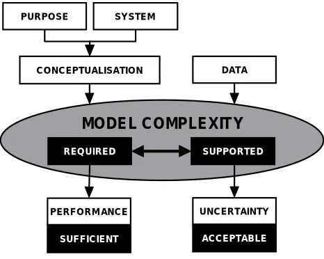
The proposed framework has been developed to investigate the appropriate balance between required levels of complexity in model structures and those which can be supported by the available data (see Fig. 1).

A hydrologist’s perception of a given hydrological system strongly influences the level of conceptualisation that must be translated into the model structure. The importance of different system response modes (i.e. key processes that need to be simulated by the model), however, depends on the modelling purpose intended. Therefore, the level of model structural complexity required must be determined through careful consideration of the key processes included in the model structure and the level of prediction accuracy necessary.

The level of structural complexity actually supported by the information contained within the observations is defined here simply as the number of parameters that can be identified. Other aspects of complexity like the number of model states or interactions between the state variables, or the use of non-linear components instead of linear ones, are not considered (see, e.g. Kleissen et al., 1990). Results from previous research suggest that, in the case of rainfall-runoff modelling, up to five or six parameters only can be identified from time-series of external system variables (i.e. streamflow and rainfall) using traditional single-objective calibration schemes (e.g. Wheater et al., 1986; Beven, 1989; Jakeman and Hornberger, 1993; Ye et al., 1997). Uncertainty in model parameters due to a lack of identifiability may limit significantly the use of models for purposes such as parameter regionalisation or the investigation of land-use or climate

change scenarios. This problem led to the investigation of less complicated, parsimonious model structures (e.g. Wagener et al., 2001) that represent only those response modes that are identifiable from the available data (e.g. Hornberger et al., 1985; Jakeman and Hornberger, 1993; Young et al., 1996). When using these models, careful consideration must be given to ensure that the model does not omit one or more hydrological processes important for a particular problem. A model structure that is too simple in terms of the number of processes reproduced can be unreliable outside the range of catchment conditions (i.e. climate and land use) on which it was calibrated (Kuczera and Mroczkowski, 1998). It is therefore vital to use data with a high information content to ensure that the main response modes can be observed from the data used for calibration (Gupta and Sorooshian, 1985).

Another approach to reducing parameter uncertainty, apart from a decrease in model complexity, is to increase the amount of information available to identify the model parameters. One way to achieve this is through the use of additional output variables. Examples are Kuczera and Mroczkowski (1998), who use time series of stream salinity measurements, and Seibert (1999), who uses groundwater measurements to constrain the parameter space. However, the usefulness of additional data can depend on the adequacy of the model structure investigated. Lamb et al. (1998) found that the use of one or only a few groundwater measurement points as additional output variable(s) helped to reduce the parameter uncertainty of TOPMODEL (Beven and Kirkby, 1979). The use of many (>100) points however, leads to an increase in uncertainty indicating structural problems of the model. A second approach is the improved use of the information already available; thus, Wheater et al. (1986) use different data periods to identify different parameters. The inherent multi-objective nature of this approach led to the development of a multi-objective calibration framework introduced by Gupta et al. (1998b) for estimating model parameter values and evaluating model structural insufficiencies. In this way, different characteristics of an output time series can be used to provide additional information. In certain applications, time-series system identification techniques can also be used to improve the identifiability of model parameters and to guide the model structure identification procedure (Young, 1984; Young et al., 1996).

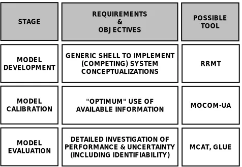
The task is, therefore, to balance the performance of the model and the identifiability of its parameters. The analytical framework proposed here to address this problem can be divided into three major stages: model development, model calibration and model evaluation. Within each stage, tools are developed and applied to meet specific goals aimed at PUR PO SE SY STEM

C O N C EPTU ALISATIO N D ATA

MO D E L C O MP LE X IT Y

R EQ U IR ED SUPPO R TED

PER F O R M AN C E U N C ER TAIN TY

SUF F IC IENT ACC EPTABLE

Fig. 1. The proposed framework for development and application of

achieving an overall balance. The stages and their corresponding requirements, objectives and possible tools are shown in Fig. 2 and described in more detail below.

Model development

The first major stage is the development of a model structure of appropriate complexity with respect to performance and associated uncertainty. This structure should be a function of (Wagener, 1998):

l the modelling purpose,

l the characteristics of the hydrological system, l the data available.

The recognition of the need for flexible model structures has led to the development of generic modelling frameworks (e.g. Woods and Ibbitt, 1993; Overland and Kleeberg, 1993; Leavsley, 1998). These systems allow the user to test the suitability of different model components and to combine them in a modular fashion. This suitability can be measured in terms of model performance (usually the achieved objective function values) and in terms of the uncertainty of the model parameters (resulting from a lack of identifiability) using different techniques as described later. New components can be added easily if none of the available components fulfils the requirements.

A Rainfall-Runoff Modelling Toolbox (RRMT, see Fig. 3) has been developed within the scope of a model regionalisation project to produce parsimonious, lumped

model structures with a high level of parameter identifiability (Wagener et al., 1999, 2001). Such identifiability is crucial if relationships between the model parameters representing the system and catchment characteristics (e.g. dominant soil types, land use, etc.) are to be established. RRMT is a modular framework that allows its user to implement different model structures to find a suitable balance between model performance and parameter identifiability. Model structures that can be implemented are lumped, relatively simple (in terms of number of parameters), and of conceptual or hybrid metric-conceptual type (Wheater et al., 1993). All structures consist of a moisture accounting and a routing module.

Model calibration

Most hydrological model structures currently used can be classified as conceptual (Wheater et al., 1993) as described earlier in the text. The algorithms used in these structures contain parameter values that often do not have a direct physical interpretation and therefore cannot be measured in the field. Instead, they must be estimated using a calibration procedure whereby the model parameters are adjusted until the system output and the model output show an acceptable level of agreement. Typically, the agreement is measured using an objective function (i.e. some aggregation function of the model residuals), usually supported by visual inspection of the calculated time series. The model (a model structure and parameter set combination) producing the best performance is commonly assumed to be representative of the natural system under investigation.

Automatic search algorithms are applied for calibration to overcome the time-consuming procedure of manual M O DEL

DEVELO PM EN T

REQ UIREM EN TS & O B JEC TIVES

PO SSIBLE TO O L

M O DEL CALIBR ATIO N

STAG E

M O DEL EVALU ATIO N

RR M T

M O CO M -UA

M C AT, G LUE DETAILED INVESTIG ATIO N O F

PERF O RM ANC E & UN CER TAIN TY (IN CLU DIN G ID ENTIF IABILITY )

"O PTIM UM " U SE O F AVAILABLE INF O R M ATIO N G ENER IC SHELL TO IM PLEM ENT

(CO M PETING ) SY STEM CO NCEPTU ALIZATIO N S

Fig. 2. The different stages, requirements and objectives for these

stages and proposed tools to use within them are shown. The following tools are suggested: the Rainfall-Runoff Modelling Toolbox (RRMT), the Multi-Objective COMplex evolution (MOCOM) algorithm of the University of Arizona (UA), the Monte-Carlo Analysis Toolbox (MCAT, and the Generalised Likelihood

Uncertainty Estimation (GLUE) method.

HY BR ID M O D EL AR CH ITECTU RE O PTIM IZATIO N

M O DU LE

VISU AL ANALY SIS

M O DU LE

O F F -LIN E DATA PRO C ESSIN G

M O DU LE

M O ISTUR E ACC O UN TING

M O DU LE

RO UTIN G M O DU LE ER

P T PET

AET

M O ISTUR E STATUS

Q

G U I

Fig. 3. The system architecture of the Rainfall-Runoff Modelling

Toolbox (RRMT). The input and output variables shown in the figure are: the precipitation P, the temperature T, the potential

evapotranspiration PET, the actual evapotranspiration AET, the effective rainfall ER, and the simulated streamflow Q. The user can

calibration. However, single-criterion algorithms have the disadvantage that their result is fully dependent on one objective function. This can lead to solutions fitting one aspect of the observed hydrograph at the expense of another. To address this problem, a multi-criteria calibration approach is proposed by Gupta et al. (1998b). In this approach, an automatic search of the feasible parameter space is used to find the set of solutions (the so-called “Pareto optimal” region) which simultaneously optimises several user-selected criteria that measure different aspects of the closeness of model output and data. This results quickly in several viable solutions, reflecting the range of different ways in which the hydrograph can be simulated with different kinds of “minimal” error (Yapo et al., 1998; Gupta et al., 1998b; Boyle et al., 2000). The Multi-Objective COMplex evolution (MOCOM-UA) algorithm (Yapo et al., 1998) is a general-purpose global optimisation algorithm capable of optimising a model population simultaneously with respect to different objective functions in a single optimisation run. It is based on an extension of the SCE-UA population evolution method (Duan et al., 1992, 1993, 1994). A detailed description and explanation of the method are given in Yapo et al. (1998) and so will not be repeated at length here.

In brief, the MOCOM-UA method involves the initial selection of a population of p points distributed randomly throughout the s-dimensional feasible parameter space. In the absence of prior information about the location of the (Pareto) optimum, a uniform sampling distribution is used. For each point the multi-objective vector F is computed, and the population is ranked and sorted using a Pareto-ranking procedure suggested by Goldberg (1989), i.e. within the population of a certain rank it is not possible to find a parameter set which is better than another with respect to all objective functions. Simplexes of s + 1 points are then selected from the population according to a robust rank-based selection method (Whitley, 1989). A multi-objective extension of the downhill simplex method (Nelder and Mead, 1965) is used to evolve each simplex in a multi-objective improvement direction. Iterative application of the ranking and evolution procedures causes the entire population to converge towards the Pareto optimum. The procedure terminates automatically when all points in the population become non-dominated, i.e. of rank one. Experiments conducted using standard synthetic multi-objective test problems have shown that the final population provides a fairly uniform approximation of the Pareto solution space (Yapo et al., 1998; Bastidas, 1998).

Model evaluation

The model evaluation stage requires the detailed investigation

of model performance, parameter identifiability, model structure suitability and prediction uncertainty. A variety of methods is necessary to address the different evaluation aspects. The understanding of model behaviour and performance gained from this stage increases the transparency of the model’s behaviour and helps to assess the reliability of the modelling results.

The Monte-Carlo Analysis Toolbox (MCAT; Wagener et al., 1999, 2001) is a collection of MATLAB (Mathworks, 1996) analysis and visualisation functions integrated through a graphical user interface. The toolbox can be used to analyse the results from Monte-Carlo parameter sampling experiments or from model optimisation methods that are based on population evolution techniques, for example, the SCE-UA or the MOCOM-UA algorithms. Although this toolbox has been developed within the context of ongoing hydrological research, all functions can be used to investigate any dynamic mathematical model.

Functions contained in MCAT include an extension of the Regional Sensitivity Analysis (RSA, Spear and Hornberger, 1980) by Freer et al. (1996), various components of the Generalised Likelihood Uncertainty Estimation (GLUE) method (Beven and Binley, 1992; Freer et al., 1996), options for the use of multiple-objectives for model assessment (Gupta et al., 1998b; Boyle et al., 2000), and plots to analyse parameter identifiability and interaction.

Rainfall-runoff modelling example

An example from the field of rainfall-runoff modelling is used to demonstrate how the proposed framework can be applied. The data and model structure selected for the case study are described briefly and examples of possible applications of the tools for model calibration and evaluation are shown.

DATA AND MODEL STRUCTURE

The Leaf River catchment (1950 km2_{) located north of}

Collins, Mississippi, USA, which has been investigated extensively (e.g. Brazil and Hudlow, 1981; Sorooshian et al., 1983) is selected for this study. Forty consecutive years (WY 1948-88) of data (daily precipitation, streamflow, and potential evapotranspiration estimates) are available for this catchment, representing a wide variety of hydrological conditions. An 11-year period (WY 1952-1962 inclusive) is used here.

identical, for the quick and a single reservoir for the slow response) in parallel as a routing component (Fig. 4). The rainfall excess model is described in detail by Moore (1985, 1999). The model assumes that the soil moisture storage capacity, c, varies across the catchment and, therefore, that the proportion of the catchment with saturated soils varies over time. The spatial variability of soil moisture capacity is described by the following distribution function

F(c) = 1 –(1–c(t)/CMAX)BEXP _{0<c(t)< CMAX (1)}

The structure requires the optimisation of five parameters: the maximum storage capacity in the catchment, CMAX [L], the degree of spatial variability of the soil moisture capacity within the catchment, BEXP [-], the factor distributing the flow between the two series of reservoirs, ALPHA [-], and the residence times of the linear reservoirs, Kq [T] and Ks [T]. The actual evapotranspiration is equal to the potential value if sufficient soil moisture is available; otherwise it is equal to the available soil moisture content.

CALIBRATION SCHEME AND PERFORMANCE CRITERIA

Traditional automatic calibration schemes use single value objective functions such as the Root Mean Square Error (RMSE),

(2)

where q_tsim _{is the simulated streamflow at time step t, q} t

obs _is

the corresponding observed streamflow, and N is the number of flow values available.

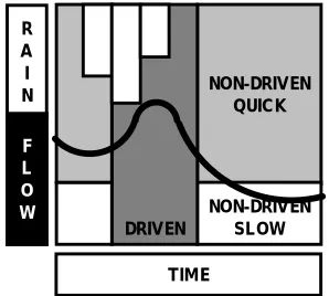
In this example, however, a partitioning scheme suggested by Boyle et al. (2000) to define objective functions based on the different response modes of the hydrological system is utilised. The approach is based on the reasonable assumption that the behaviour of the catchment is inherently different during periods “driven” by rainfall and periods without rain. Further, the periods immediately following the cessation of rainfall and dominated by interflow can be distinguished from the later periods that are dominated by baseflow. The streamflow hydrograph can, therefore, be partitioned into three components (Fig. 5), “driven” (Q_D),

ER 1 (t)

K q K q K q

K s

P(t) AET(t)

st

o

ra

g

e

ca

p

aci

ty

F (c ) S(t) C M AX

ALP HA

ER 2 (t) _{Q (t)}

1 0

c (t)

Fig. 4. The model structure used in the rainfall-runoff modelling example. Effective rainfall (ER1(t) and ER2(t)) is produced

depending on the current catchment moisture state described by the storage capacity distribution function F(c). The parameter CMAX describes the maximum storage capacity in the catchment. The effective rainfall is distributed with respect to parameter ALPHA and either routed through three linear reservoirs with residence time Kq in series, or a single reservoir with residence time Ks. Variable Q(t) is the resulting streamflow at time step t. The remaining variables are the storage S(t), the precipitation input P(t),

and the actual evapotranspiration AET(t).

NON-DRIV EN QUIC K

NON-DRIV EN SL OW DRIV EN

T IM E R

A I N

F L O W

Fig. 5. Hydrograph segmentation into three components based on

different response modes of the catchment system, i.e. “driven” (Q_D - dark grey), “non-driven quick” (QQ - light grey) and “non-driven

“non-driven quick” (Q_Q), and “non-driven slow” (Q_S). The time steps corresponding to each of these components are identified through an analysis of the precipitation data and the time of concentration for the catchment. The time steps with non-zero rainfalls, lagged by the time of concentration for the catchment, are classified as driven. Of the remaining (non-driven) time steps, those with streamflow lower than a certain threshold value (e.g., mean of the logarithms of the flows) are classified as non-driven-slow, and the rest are classified as non-driven-quick. The model performance during these three periods (Q_D, Q_Q, and Q_S) is estimated by calculating the RMSE (FD, FQ, FS) separately over each period.

The primary motivation for partitioning the non-driven flows into a quick and a slow component is to identify the periods of hydrograph recession or “baseflow” behaviour from the rest of the non-driven flow. For the purposes of this study, a simple systematic approach (threshold flow value) is chosen to identify these periods. The sensitivity of the threshold values to the identification of the recession periods is investigated prior to the multi-criteria optimisation. Several different threshold values are tested (median of flows, mean of flows, mean of log of flows, etc.) to determine which value provided the best representation of the recession flows as determined through visual inspection of the observed hydrograph (results not shown here). The mean of the log of the flows provided the “best” estimate of the recession periods for this data set. There are certainly other, possibly more accurate, methods (e.g., visual inspection, water balance and ground water recharge methods) to identify these recession periods; however, these have to be the subject of future studies. Presumably, the more accurately the characteristic features of the catchment are identified, the more informative the analysis.

Two calibration methods, Uniform Random Search (URS) and MOCOM-UA, are used to explore the parameter space of the model. The URS method consists of 5000 parameter sets randomly sampled from the feasible parameter ranges based on a uniform distribution. The Pareto optimal solution space for the three criteria is estimated with 500 solutions using the MOCOM-UA multi-criteria optimisation algorithm (Yapo et al., 1998).

SENSITIVITY AND IDENTIFIABILITY ANALYSIS

A modification of the RSA approach introduced by Freer et al. (1996) is used to inspect visually the sensitivity of the different parameters with respect to the response mode of the system. This methodology was introduced originally to identify insensitive parameters which subsequently would be fixed or eliminated. However, it can also be used to visualise the link between parameter sensitivity and system

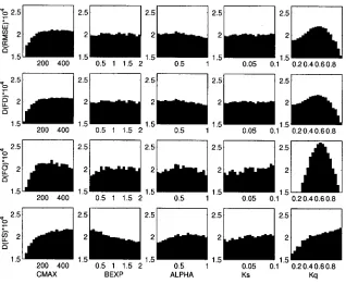
response modes (Dunne, 1999; Wagener et al., 1999). Freer et al. (1996) split the parameter population, derived from a URS procedure and ranked with respect to their objective function values, into ten groups of equal size and plotted the cumulative distribution of the parameters in each group with respect to the transformed measure of performance. The measures are transformed so that higher values indicate better models and they are divided by their sum so that they add up to unity. An insensitive parameter would produce a straight line, while differences in form and separation of the resulting curves indicate parameter sensitivity. Splitting the population into ten groups, instead of just two as in the original method, avoids the selection of a threshold value between behavioural and non-behavioural parameter sets, and increases the information gained by the analysis. Figure 6 visualises the results derived for this study with the shading ranging from light grey (best performing group) to black (worst performing group). The figure shows the sensitivity of the model parameters based on the RMSE, first used as an overall measure for the whole calibration period (first row), and subsequently for the three measures of the different response modes (FD, FQ, FS).

The overall RMSE and the FD measures show very similar behaviour, indicating that they retrieve similar information from the observed data. The curves produced using these two measures are markedly different from those resulting from the FS measure. The sensitivity of the BEXP parameter is considerably higher during periods of non-driven slow response, i.e. FS. The sensitivity of Kq is relatively high for all measures. However, the shape of the cumulative curves of this parameter for the FS measure is different. This indicates that the parameter population conditioned on this measure results in a different distribution than when the other measures are used. The sensitivity plots for the parameter ALPHA are similar for all objective functions, suggesting that this parameter is equally important for the correct reproduction of the system behaviour during all response modes. The same is observed for parameter CMAX.

Fig. 6. Regional Sensitivity Analysis plots showing the varying sensitivity of the model

parameters depending on the response mode of the hydrological system: (1st _{row) Single} overall measure (RMSE), (2nd _{row) measure for “driven” period (FD), (3}rd _{row) measure} for “non-driven quick” period (FQ), and (4th _{row) measure for “non-driven slow” period} (FS). Lighter colours indicate groups of better performing parameters, while darker

colours indicate less well performing parameters.

Fig. 7. The objective functions are rescaled so that the best performing parameter assumes the highest

value and the sum of all values equals one. Splitting each parameter range subsequently into 20 bins of equal width and calculating the sum of all measures in each bin leads to the parameter

this case initially uniform, parameter populations conditioned on the different objective functions.

Some variation in the distributions derived through the use of the different measures can be seen. The parameter BEXP shows relatively uniform distributions except when being conditioned on FS, where small values show better performance. The parameter population of Kq on the other hand shows a very distinct peak for the FQ objective function. However, higher values of this parameter are favoured when the FS objective function is used to obtain a better fit at the beginning of the recession periods of the hydrograph. ALPHA shows relatively similar distributions for all measures, which is in line with the result of the sensitivity analysis (Fig. 6) in which the parameter is sensitive for all objective functions.

Figure 7 shows that the use of different measures can lead to an improvement in judging the performance of a parameter over its range. A parameter showing little variation using

one measure may reveal a distinct peak in its distribution when using an objective function based on residuals from a different response period. This is caused by the often varying importance of model components, and therefore parameters, to reproduce the system behaviour during different response modes.

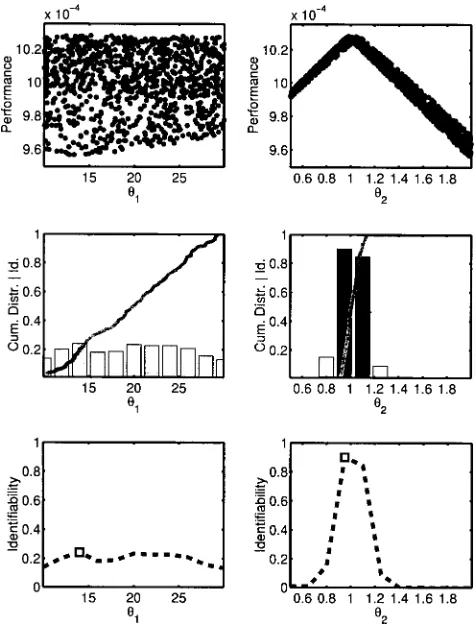
A different measure of the identifiability of a parameter, and therefore the uncertainty related to this parameter, is defined in Fig. 8. A synthetic example is used whose parameters are not related to the model structures used here. The top row of this figure shows two scatter plots of two different parameter populations derived from a URS procedure. Parameter q

1 is unidentifiable, i.e. good

performing parameters appear at very different locations in the feasible parameter space. Parameter q

2 on the other hand

is very identifiable with a distinct peak. Plotting the cumulative distribution of the 100 best performing parameter sets used in the example application (since only the top of

Fig. 8. The top row shows scatter plots of two parameter populations derived from a uniform random search.

The performance is measured by the root mean square error, transformed so that better performing models are indicated by higher values and the measures sum to unity. Parameter q₁ is unidentifiable, while parameter q₂ is very identifiable. The top population (e.g. best performing 100 models) can be used to derive a cumulative distribution with respect to their performance. Splitting the parameter range into ten bins and calculating the gradient of the cumulative distribution within each results in the (rescaled) gradient distribution shown as bars in the middle row. The bottom row shows the (rescaled) gradient distribution as a line with the marker

the population is interesting for an analysis of the identifiability), leads to the plots shown in the middle row of Fig. 8. The unidentifiable parameter q

1 produces a straight

line between the bottom left and the top right corner of the plot. The other parameter produces a much steeper line over only part of the parameter space. Splitting each parameter range into a number of equally spaced bins (e.g. 10) and calculating the gradient of the cumulative distribution within each bin gives a measure of identifiability of the parameter. The gradients are plotted as bars. Additionally, a colour coding is used, with darker colours indicating higher gradients. The middle left plot shows that the resulting gradients of parameter q

1 are low and almost equal over the

whole parameter range. The gradients of parameter q₂ are much larger and indicate where a peak is occurring on the response surface and how pronounced it is. The gradient of the cumulative distribution of each parameter can therefore be used as a measure of its identifiability. The bottom row of Fig. 8 shows the gradient distributions of the two parameters as lines, with the top value indicated by a marker.

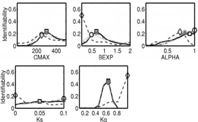
This measure is used to analyse the identifiability of the model parameters. The results are given in Fig. 9. The first plot shows that the level of identifiability of CMAX is relatively similar for all objective functions. Parameter BEXP is more identifiable when using FS. The identifiability values, i.e. the gradients, are higher during the non-driven slow periods and small values of this parameter perform better. Parameter ALPHA shows a reasonable consistency in the level of identifiability through all measures. The identifiability of Ks is slightly higher during the non-driven

slow periods (FS). Parameter Kq shows very high levels of identifiability for all objective functions. The locations of the peaks are almost identical apart from the conditioning on FS, which favours higher values of the parameter.

Figure 9 shows again that the main difference can be found between FS and the remaining measures. The measures FD, FQ, and RMSE seem to contain similar information for this data set. However, the use of different measures can be beneficial for the identifiability of parameters as is demonstrated in the cases of BEXP and Ks.

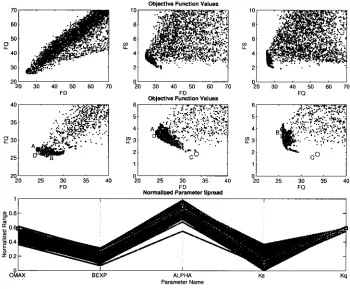
A two-dimensional projection of the three-dimensional objective function space (FD, FQ, FS) gives further insights (Fig. 10, 1st _{and 2}nd _{row). The light grey dots indicate the}

500 Pareto solutions determined with the MOCOM-UA algorithm whereas the black dots show the 5000 URS results. The 2nd _{row shows the region of the Pareto solution in greater}

detail with the best solutions highlighted (A for FD, B for FQ, C for FS, D for overall RMSE). These plots illustrate clearly the inability of the model to match all three aspects of the hydrograph simultaneously, and reveal that the trade-offs in fitting the three hydrograph components are quite significant. However, the trade-off between FD (A) and FQ (B) is relatively small, which is also indicated by the relatively high degree of correlation of the Monte-Carlo results (top left plot). In addition the best FD and overall RMSE solutions are very similar with respect to the three criteria indicating that these two measures contain very similar information about the parameters of this model. The normalised (over the initial parameter uncertainty range) parameter plot, presented in the bottom row of Fig. 10, shows the variability

Fig. 9. The distribution of gradients for the different parameters and the different

objective functions is shown. The markers indicate the highest gradient values for FD (rectangle), FQ (circle), FS (diamond) and RMSE (star), also ranging from dark (FD)

in the parameter values for the 500 Pareto optimal solutions (indicated by the light grey lines). Each line on the graph represents one of the parameter sets. Notice that the parameter uncertainty has been reduced significantly by the multi-criteria optimisation compared to the initial feasible range, particularly for Kq. Also notice that the parameter values for the best FD, FQ, and RMSE solutions are, in general, in a different region of the parameter space than the best solution for the FS criteria (indicated by the dashed line).

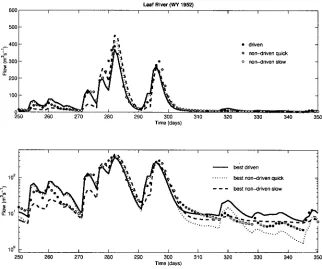
Figure 11 presents the model output results for a 100-day portion of the calibration period derived using the results of the calibration with the MOCOM-UA algorithm. The minimal FD and FQ solutions tend to fit the peaks better at the expense of over- and underestimating the recessions respectively. The minimal FQ solution also captures the shape of the falling limb, corresponding with time steps classified as “non-driven quick”, better than the other two solutions. The minimal FS solution on the other hand fits the long recession limbs of the hydrograph better (see log-scale plot at bottom), while it often seriously over- or underestimates

the peaks. The model does generally have some trouble matching the flows for days 250 through 270. This could be due to model structural error, i.e. the model’s inability to track the soil moisture in the long dry period preceding these rainfall events. Another possibility is that the precipitation data during this time period is erroneous, i.e. it may not be representative of the precipitation rates throughout the catchment.

This simple example demonstrates how the aggregation of the residuals over the whole calibration period results in a loss of information relating to parameter sensitivity and identifiability, model performance, and model structural insufficiencies. Additional insight is gained from the hydrograph split performed here.

The advantages of a multi-objective framework based on system response modes make it especially suitable for comparison studies since it allows us to attribute the model performance during different system response modes to different model components, i.e. in this case the moisture accounting and the routing components. A certain model

Fig. 10. Two-dimensional projections of the three dimensional objective function space (1st _{and 2}nd _row show 500 Pareto solutions and 5000 parameter sets randomly sampled from a uniform distribution). The markers correspond to the best points with respect to FD (A), FQ (B), FS (C), and overall RMSE (D). The 3rd _{row shows the normalised parameter space. The grey lines show the 500 Pareto solutions, the} three black lines are solutions A (FD, solid), B (FQ, dotted), and C (FS, dashed). The squares indicate

structure might perform better during “driven” periods because of a superior moisture accounting component, while another model structure containing a more appropriate slow flow routing component could result in higher performance during “non-driven slow” periods. A single-objective framework does not allow the comparison of model components and consequently important information relevant to identifying the most suitable model structure is lost. Boyle et al. (2001) use this advantage of multi-objective comparison studies in their research evaluating the benefit of “spatial distribution” of model input (precipitation), structural components (soil moisture and streamflow routing computations) and surface characteristics (parameters) with respect to the reproduction of different response modes of the catchment system.

MODEL STRUCTURE COMPARISON

A second model structure is introduced to demonstrate the advantages of multi-objective comparisons. This structure is a simplified version of the model described before. A single store with a rainfall excess mechanism is used as moisture accounting component, instead of a distribution of stores as in the first structure. The store is described by its size, CMAX [L]. The evapotranspiration losses of the store are again equal to the potential rate as long as soil moisture is available. The

remaining structural components are identical to the ones of the earlier model structure shown in Fig. 4 and are defined by three parameters, ALPHA [-], Kq [T], and Ks [T]. This structure is referred to as the simple model, while the initial structure is referred to as the complex model in the remaining text.

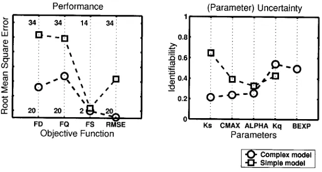
The results of the comparison are shown in Fig. 12. The left graph shows a comparison in performance between the two structures as derived from the calibration with the MOCOM-UA algorithm. The objective functions used are identical to the ones applied when analysing the individual model structure earlier in the text. The traditional, overall measure of performance RMSE, indicates that the complex model structure is superior to the simple one. However, when analysing the performance in more detail, one can see that both structures are almost equally good during the non-driven slow periods (FS). The complex model structure is able to fit the driven and non-driven quick periods better, with the largest difference occurring during the driven period. This result shows the initial insight gained by a more detailed analysis. The model structures have identical components to fit the slow catchment drainage (Q_S) and therefore produce similar results. The fact that this is not the case during the quick catchment drainage (Q_Q) can be attributed to the larger importance of the moisture accounting component in fitting

Fig. 11. Hydrograph range produced by the 500 Pareto solutions (grey region), and the

this part of the hydrograph, and that it is easier to separate out the slow recession periods.

The evaluation of the model performance should, if possible, also include objective functions tailored to fit the specific purpose of the model. An example is the use of the model to investigate available water quantities for abstraction purposes. Assuming that abstraction can only take place during periods when the water level is above minimum environmentally acceptable flow and below a maximum water supply abstraction rate allows the definition of a specific objective function (Lees and Wagener, 2001). This measure would only aggregate the residuals of the selected period and can give important information about how a model performs with respect to the anticipated task. However, it is important to mention that this should never be the only evaluation criterion.

The right-hand graph of Fig. 12 shows the uncertainty in estimating the parameters of the two models, i.e. in terms of their identifiability. The highest identifiability values for each of the parameters of the complex model are taken from Fig. 9. The identifiability values for the simple model parameters are derived in an identical way. It can be seen that the simple model structure shows overall a higher degree of parameter identifiability. Introducing an additional parameter, BEXP, generally reduces the identifiability through its interaction with the other parameters. The increase in model performance is therefore obtained at the cost of decreasing identifiability, and therefore increasing parameter uncertainty.

The trade-off between improvement in performance and

reduction in identifiability should be considered, amongst other things, when selecting a model structure for a specific purpose. A simpler model structure, representing a smaller number of processes, might for example be more suitable for regionalisation purposes. The type of analysis shown supports the model selection process.

Conclusions

A rigorous approach to the development and evaluation of hydrological models is required, balancing prior information, model complexity, and parameter and output uncertainty. The framework presented here incorporates those aspects.

The simple example shows that accepting the multi-objective nature of model calibration and integrating it into the modelling process increases the amount of information retrieved from the model residuals to (1) find the parameter population necessary to fit all aspects of the observed output time-series (albeit separately), (2) increase the identifiability of the model parameters, and (3) assess the suitability of the model structure to represent the natural system (i.e. identify model structural insufficiencies). The methodology has general applicability. The global and multi-objective optimisation algorithm MOCOM-UA, in this respect, has already been applied successfully to rainfall-runoff (Gupta et al., 1998b; Yapo et al., 1998; Boyle et al., 2000), to more complex, coupled Soil-Vegetation-Atmosphere-Transport (SVAT, Bastidas et al., 1998; Gupta et al., 1998a), and to water-quality (Meixner et al., 2000) models.

Fig. 12. The two model structures compared in terms of performance and uncertainty in

(identifiability of) their parameters. The left plot shows the root mean square error values of the two structures with respect to the different objective functions used. A smaller value therefore indicates a higher performance. The plot on the right shows the identifiability of the parameters of the two structures. A higher value indicates a higher degree of identifiability and therefore reduced uncertainty. The identifiability value for each parameter is the highest derived from the different objective functions as shown in Fig. 9

The methods and tools described here complement each other allowing for improved development and application of hydrological models in a multi-objective framework, which makes optimal use of available information. This framework is easily extendable to more complex hydrological models including coupled models with multiple outputs.

The two Matlab toolboxes, RRMT and MCAT, are available from the Imperial College web-site at http:// ewre.cv.ic.ac.uk/, while the code for the MOCOM-UA algorithm is available from Hoshin V. Gupta (via [email protected]).

Acknowledgements

Work described in this paper was partially funded by NERC grant GR3/11653. The authors appreciate the critical comments of N. McIntyre and the reviewers which led to improvements in the paper.

References

Bastidas, L.A., 1998. Parameter estimation for hydrometeorological

models using multicriteria methods, Ph.D. Dissertation, Dep.

Hydrol. Water Resour., The University of Arizona.

Bastidas, L.A., Gupta, H.V., Sorooshian, S., Shuttleworth, W.J. and Yang, Z.L., 1998. Sensitivity analysis of a land surface scheme using multicriteria methods, J. Geophys. Res., 104, 19481-19490. Beven, K.J., 1989. Changing ideas in hydrology – The case of

physically-based models, J. Hydrol., 105, 157-172.

Beven, K.J. and Binley, A.M., 1992. The future of distributed models: Model calibration and uncertainty prediction, Hydrol.

Process., 6, 279-298.

Beven, K.J. and Kirkby, M.J., 1979. A physically based, variable contributing area model of basin hydrology, Hydrol. Sci. Bull., 24, 43-69.

Boyle, D.P., Gupta, H.V. and Sorooshian, S., 2000. Towards improved calibration of hydrologic models: Combining the strengths of manual and automatic methods, Water Resour. Res., 36, 3663-3674.

Boyle, D.P., Gupta, H.V., Sorooshian, S., Koren, V., Zhang, Z. and Smith, M., 2001. Towards improved streamflow forecasts: The value of semi-distributed modelling, Submitted to Water Resour.

Res.

Brazil, L.E. and Hudlow, M.D., 1981. Calibration procedures used with the National Weather Service Forecast System. In: Water

and related land resources systems (Eds. Y.Y. Haimes and J.

Kindler), Pergamon, New York, 457-466.

Duan, Q., Gupta, V.K. and Sorooshian, S., 1992. Effective and efficient global optimisation for conceptual rainfall-runoff models, Water Resour. Res., 28, 1015-1031.

Duan, Q., Gupta, V.K. and Sorooshian, S., 1993. A shuffled complex evolution approach for effective and efficient global minimization, J. Optimiz. Theor. Appl., 76, 501-521.

Duan, Q., Sorooshian, S. and Gupta, V.K., 1994. Optimal use of the SCE-UA global optimization method for calibrating catchment models, J. Hydrol., 158, 265-284.

Dunne, S.M., 1999. Imposing constraints on parameter values of a conceptual hydrological model using baseflow response, Hydrol.

Earth System. Sci., 3, 271-284.

Freer, J., Beven, K.J. and Ambroise, B., 1996. Bayesian estimation of uncertainty in runoff prediction and the value of data: An application of the GLUE approach, Water Resour. Res., 32, 2161-2173.

Goldberg, D.E., 1989. Genetic algorithms in search, optimization

and machine learning, Addison-Wesley, Reading, Mass.

Gupta, V.K. and Sorooshian, S., 1985. The relationship between data and the precision of parameter estimates of hydrologic models, J. Hydrol., 81, 57-77.

Gupta, H.V., Bastidas, L.A., Sorooshian, S., Shuttleworth, W.J. and Yang Z.L., 1998a. Parameter estimation of a land surface scheme using multicriteria methods, J. Geophys. Res., 104, 19491-19503. Gupta, H.V., Sorooshian, S. and Yapo, P.O., 1998b. Towards improved calibration of hydrologic models: Multiple and noncommensurable measures of information, Water Resour. Res., 34, 751-763.

Hornberger, G.M., Beven, K.J., Cosby, B.J. and Sappington, D.E., 1985. Shenandoah watershed study: Calibration of the topography-based, variable contributing area hydrological model to a small forested catchment, Water Resour. Res., 21, 1841-1850. Jakeman, A.J. and Hornberger, G.M., 1993. How much complexity is warranted in a rainfall-runoff model? Water Resour. Res., 29, 2637-2649.

Kleissen, F.M., Beck, M.B. and Wheater, H.S. 1990. The identifiability of conceptual hydro-chemical models. Water

Resour. Res., 26, 2979-2992.

Kuczera, G. and Mroczkowski, M., 1998. Assessment of hydrologic parameter uncertainty and the worth of multiresponse data, Water

Resour. Res., 34, 1481-1489.

Lamb, R., Beven, K.J. and Myrabo, S., 1998. Use of spatially distributed water table observations to constrain uncertainty in a rainfall-runoff model. Adv. Water Resour., 22, 305-317. Leavsley, G., 1998. The modular modelling system (MMS) – A

modelling framework for multidisciplinary research and operational applications, http: //wwwbrr.cr.usgs.gov/ projects/

SW_precip_runoff/mms/.

Lees, M.J. and Wagener, T., 2000. HYCOM rainfall-runoff

modelling of Bewl-Darwell reservoir source rivers. Unpublished

report to Southern Water, UK.

Mathworks, 1996. Matlab – Reference guide, The Mathworks Inc., Natick, MA.

Meixner, T., Bastidas, L.A., Gupta, H.V. and Bales, R.C., 2000. Multi-Criteria Parameter Estimation for Models of Stream Chemical Composition, Submitted to Water Resour. Res. Moore, R.J., 1985. The probability-distributed principle and runoff

production at point and basin scales, Hydrol. Sci. J., 30, 273-297.

Moore, R.J., 1999. Real-time flood forecasting systems: Perspectives and prospects. In: Floods and landslides: Integrated

risk assessment (Eds. R. Casale and C. Margottini), Springer,

Berlin, 147-189.

Nelder, J.A. and Mead, R., 1965. A simplex method for function minimization, Comp. J., 7, 308-313.

Overland, H. and Kleeberg, H.-B., 1993. Moeglichkeiten der Abflussmodellierung unter Nutzung von Geoinformations systemen, Mitteilungen des Instituts fuer Wasserwesen, 45, Neubiberg.

Seibert, J., 1999. Conceptual runoff models - fiction or representation of reality? Acta Univ. Ups., Comprehensive

Summaries of Uppsala Dissertations from the Faculty of Science and Technology 436. 52 pp. Uppsala.

Spear, R.C. and Hornberger, G.M., 1980. Eutrophication in Peel Inlet, II, Identification of critical uncertainties via generalized sensitivity analysis, Water Resour. Res., 14, 43-49.

Wagener, T., 1998. Developing a knowledge-based system to support

rainfall-runoff modelling, MSc. Thesis, Dep. Civil Eng., Delft

University of Technology, NL.

Wagener, T., Lees, M.J. and Wheater, H.S., 1999. A generic rainfall-runoff modelling toolbox, EOS Trans. AGU, 80, Fall Meet. Suppl., F203.

Wagener, T., Lees, M.J. and Wheater, H.S., 2001. A toolkit for the development and application of parsimonious hydrological models, To appear in: Mathematical models of small watershed

hydrology – Volume 2 (Eds. Singh, Frevert and Meyer), Water

Resources Publications LLC, USA.

Wheater, H.S., Bishop, K.H. and Beck, M.B., 1986. The identification of conceptual hydrological models for surface water acidification, Hydrol. Process., 1, 89-109.

Wheater, H.S., Jakeman, A.J. and Beven, K.J., 1993. Chapter 5 – Progress and directions in rainfall-runoff modelling, In: Modelling

change in environmental systems (Eds. A.J. Jakeman, M.B. Beck

and M.J. McAleer), Wiley, Chichester, UK, 101-132.

Whitley, D., 1989. The genitor algorithm and selection pressure:

Why rank-based allocation of reproductive trials is best, Paper

presented at Third International Conference on Genetic Algorithms.

Woods, R.A. and Ibbitt, R.P., 1993. Building a rainfall-runoff modelling system: Ideas and practice, In: International congress

on modelling and simulation – Proceedings – Volume I. (Eds.

M.J. McAleer and A.J. Jakeman) Uniprint, University of Western Australia, 25-30.

Yapo, P.O., Gupta, H.V. and Sorooshian, S., 1998. Multi-objective global optimization for hydrologic models, J. Hydrol., 204, 83-97.

Ye, W., Bates, B.C., Viney, N.R., Sivapalan, M. and Jakeman, A.J., 1997. Performance of conceptual rainfall-runoff models in low-yielding ephemeral catchments, Water Resour. Res., 33, 153-166. Young, P.C., 1984. Recursive estimation and time-series analysis,

Springer-Verlag, Berlin.

Young, P.C., Parkinson, S. and Lees, M.J., 1996. Simplicity out of complexity in environmental modelling: Occam’s razor revisited,