https://doi.org/10.5194/hess-23-3843-2019 © Author(s) 2019. This work is distributed under the Creative Commons Attribution 4.0 License.
Using the maximum entropy production approach to integrate
energy budget modelling in a hydrological model
Audrey Maheu1, Islem Hajji2, François Anctil2, Daniel F. Nadeau2, and René Therrien3 1Département des sciences naturelles, Université du Québec en Outaouais, Ripon, J0V 1V0, Canada 2Département de génie civil et de génie des eaux, Université Laval, Québec, G1V 0A6, Canada 3Département de géologie et de génie géologique, Université Laval, Québec, G1V 0A6, Canada Correspondence:Audrey Maheu ([email protected])
Received: 21 December 2018 – Discussion started: 31 January 2019
Revised: 18 June 2019 – Accepted: 17 August 2019 – Published: 20 September 2019
Abstract. Total terrestrial evaporation, also referred to as evapotranspiration, is a key process for understanding the hydrological impacts of climate change given that warmer surface temperatures translate into an increase in the atmo-spheric evaporative demand. To simulate this flux, many hy-drological models rely on the concept of potential evapora-tion (PET), although large differences have been observed in the response of PET models to climate change. The maxi-mum entropy production (MEP) model of land surface fluxes offers an alternative approach for simulating terrestrial evap-oration in a simple way while fulfilling the physical con-straint of energy budget closure and providing a distinct es-timation of evaporation and transpiration. The objective of this work is to use the MEP model to integrate energy bud-get modelling within a hydrological model. We coupled the MEP model with HydroGeoSphere (HGS), an integrated sur-face and subsursur-face hydrologic model. As a proof of con-cept, we performed one-dimensional soil column simula-tions at three sites of the AmeriFlux network. The cou-pled model (HGS-MEP) produced realistic simulations of soil water content (root-mean-square error – RMSE – be-tween 0.03 and 0.05 m3m−3; NSE – Nash–Sutcliffe effi-ciency – between 0.30 and 0.92) and terrestrial evaporation (RMSE between 0.31 and 0.71 mm d−1; NSE between 0.65 and 0.88) under semi-arid, Mediterranean and temperate cli-mates. At the daily timescale, HGS-MEP outperformed the stand-alone HGS model where total terrestrial evaporation is derived from potential evaporation, which we computed using the Penman–Monteith equation, although both mod-els had comparable performance at the half-hourly timescale. This research demonstrated the potential of the MEP model
to improve the simulation of total terrestrial evaporation in hydrological models, including for hydrological projections under climate change.
1 Introduction
to model (McKenney and Rosenberg, 1993; Kingston et al., 2009; Donohue et al., 2010; Lofgren et al., 2011; McAfee, 2013; Hosseinzadehtalaei et al., 2016). These differences of-ten translate into large uncertainty in stream discharge pro-jections (Kay and Davies, 2008; Bae et al., 2011; Milly and Dunne, 2011; Prudhomme and Williamson, 2013; Seiller and Anctil, 2016), although some studies have demonstrated op-posite results with a relatively low sensitivity of discharge projection to PET model selection (Thompson et al., 2014; Koedyk and Kingston, 2016).
Among PET models, those that are based on temperature tend to mainly reflect changes in mean air temperature, even though temperature is not necessarily the strongest control on PET (Donohue et al., 2010; Shaw and Riha, 2011). For example, the oversensitivity of temperature-based models to surface warming has been linked to an exaggerated assess-ment of drought severity under climate change (Hoerling et al., 2012). As a result, recent studies have recommended the use of physically based PET models, such as the Pen-man model, for simulating terrestrial evaporation in climate change assessments (Hobbins et al., 2008; Sheffield et al., 2012; McAfee, 2013). However, additional data inputs (e.g. radiation, humidity and wind speed) are required to imple-ment such models, and, as opposed to the high confidence placed on temperature estimates from global climate mod-els (McMahon et al., 2015), these variables usually suffer from a lower reliability. For example, large differences per-sist between observations, reanalysis products and global cli-mate model projections of wind speed (McVicar et al., 2008; Pryor et al., 2009). Overall, a dilemma emerges for the simu-lation of PET under climate change, which involves choosing between a reliable physically based model with greater in-put data uncertainty versus an overly simplified temperature-based model with reliable input data (Ekström et al., 2007; Kay and Davies, 2008; Kingston et al., 2009).
Given these current limitations with PET models, alterna-tive approaches are needed for the simulation of terrestrial evaporation in climate change assessments. Energy budget modelling offers a physically based approach for simulating terrestrial evaporation (along with other components of the surface energy budget), with the added benefit of conserva-tion of energy that ensures a balance between incoming and outgoing energy. Land surface models provide a means to simulate both water and energy budgets, and they have been used for hydrological modelling, either by (i) coupling hy-drological and land surface models (Pietroniro et al., 2001; Maxwell and Miller, 2005; Kunstmann et al., 2008; Zabel and Mauser, 2013) or by (ii) coupling a land surface model to a routing scheme (Gaborit et al., 2017). In land surface models, terrestrial evaporation is generally estimated with a bulk aerodynamic approach (Noilhan and Planton, 1989) that relies on semi-empirical equations and requires information on vertical gradients of air temperature and humidity that can introduce substantial errors. The use of land surface models can yield small gains in hydrological modelling performance
(Livneh et al., 2011; Shi et al., 2014), but they remain com-putationally heavy.
Optimality principles, which are derived from the idea that nature organizes itself to ensure optimal functioning, provide an alternative avenue for modelling terrestrial evaporation. Maximum entropy production (MEP) is one of the optimal-ity principles put forward, and although it has yet to become an established principle, it offers a promising method to im-prove hydrological modelling (Ehret et al., 2014; Westhoff and Zehe, 2013). The MEP principle has been applied in two ways in hydrology. In the first approach, MEP is de-fined as a physical principle, which hypothesizes that an open thermodynamic system far from equilibrium can achieve a steady state at which, through self-organization, entropy is produced at the maximum possible rate. Such a dynamic equilibrium can be achieved because, as demonstrated by Paltridge (1975), a gradient drives a flux that, in turn, de-pletes the initial gradient and further reinforces it. Using this approach, MEP has been used to constrain parameters of hy-drological models (Kleidon and Schymanski, 2008; Porada et al., 2011; Westhoff and Zehe, 2013). In the second ap-proach, MEP is defined as a statistical principle and con-stitutes the most probable state of an open system (Dewar, 2005, 2009). Using the MaxEnt statistical inference algo-rithm (Jaynes, 1957), the state of MEP can be predicted by maximizing Shannon information entropy while considering constraints imposed by the available information. Both con-cepts of entropy are linked: the maximization of Shannon in-formation entropy can be used to assess the probability of a given state for any kind of system, and as such, thermo-dynamic entropy can be considered a special case of Shan-non information theory. In hydrology, Wang and Bras (2009, 2011) have used the Shannon information entropy approach to develop the MEP model of land surface fluxes, which is the topic of the present article.
oversensitiv-Table 1.Description of study sites.
US-Wkg US-Ton US-WBW
Climate Semiarid Mediterranean Temperate Köppen climate class Bsk: steppe, warm winter Csa: Mediterranean, mild with
dry, hot summer
Cfa: humid subtropical, mild with no dry season, hot summer Vegetation class Grassland Woody savanna Deciduous broadleaf forest Mean annual precipitation (mm) 407 559 1372
Mean annual temperature (◦C) 15.6 15.8 13.7
Data source Scott (2016) Baldocchi (2016) Meyers (2016)
ity to temperature and suggests that this approach should be robust in climate change assessments. Recent studies also re-ported improved performance of the MEP approach for the simulation of terrestrial evaporation when compared against the Penman–Monteith model (Hajji et al., 2018) or a mod-ified Penman–Monteith approach driven by remote sensing and reanalysis data (Xu et al., 2019). The MEP model also had a performance comparable to a complex land surface model (Canadian Land Surface Scheme – CLASS) at snow-free sites at low latitudes (Alves et al., 2019). Overall, the MEP model offers an attractive approach to improve the sim-ulation of terrestrial evaporation in hydrological modelling and to increase the robustness of streamflow projections un-der climate change. The objective of this study is thus to couple the MEP model of land surface fluxes with a hydro-logical model and perform proof-of-concept simulations at AmeriFlux sites spanning a range of climatic and vegetation conditions.
2 Study area
We selected three sites of the AmeriFlux network (Baldoc-chi et al., 2001) where the eddy covariance method is used to measure vertical water and energy fluxes (Table 1; Fig. 1). We selected sites using the following criteria: (i) measure-ments of volumetric soil water content available at different depths and for an extended period, (ii) absence of snow cover, and (iii) diversity in climates (semi-arid, Mediterranean and temperate) and types of vegetation (grassland, woody sa-vanna and deciduous broadleaf forest).
[image:3.612.54.539.85.186.2]The first site, US-Wkg, is characterized by a semi-arid cli-mate where 60 % of precipitation is concentrated in July, Au-gust and September. In 2006, a sharp transition occurred in the vegetation and the native grassland species (assemblage of grama grasses, genus Bouteloua) have been supplanted by Lehman lovegrass (Eragrostis lehmanniana), an exotic species spreading throughout the southwestern United States (Moran et al., 2009; Scott et al., 2010). The second site, US-Ton, is characterized by a Mediterranean climate, with dry summers and most precipitation occurring from October to May. The woody savanna is made up of two layers of veg-etation, each reaching peak activity at different times of the
Figure 1.Location of study sites across the conterminous United States.
year (Baldocchi et al., 2004). Trees, mainly blue oaks ( Quer-cus douglasii), are dormant during winter months, reach peak activity in the spring and then carefully regulate their water use during the dry summer period. In contrast, the under-story vegetation composed of grasses and forbs is mainly active during the rainy winter period, when water is plenti-ful. Finally, the US-WBW site is characterized by a temper-ate climtemper-ate, with precipitation relatively evenly distributed throughout the year. The mixed deciduous forest is domi-nated by oak and hickory, and vegetation is active from the spring to early autumn (April to October), with peak activity during the summer (Wilson and Baldocchi, 2000).
3 Methodology
[image:3.612.311.544.144.375.2]from the principle of maximum entropy (MaxEnt) developed by Jaynes (1957) as a general inference tool for assigning probability distributions in statistical mechanics. Wang and Bras (2009) used this statistical approach to develop the MEP model of land surface fluxes. Within the MEP model, land surface fluxes are each expressed in terms of a dissipation or entropy function, and under the constraint of conservation of energy, a unique extremum solution is found.
Dissipation functions have been postulated for land sur-face fluxes over a dry soil (Wang and Bras, 2009) and over wet soil and vegetation surfaces (Wang and Bras, 2011). For non-vegetated surfaces, bare soil evaporation (Es) is esti-mated by solving Eqs. (1) and (2) with the constraint of en-ergy conservation at the surface (Rn=G+Es+H; Wang and Bras, 2011):
Es=B(σ )H, (1)
G=B (σ ) σ
Is I0
H|H|−16, (2)
whereRn,Es,HandGare the net radiation and latent, sen-sible and ground heat fluxes at the soil surface (W m−2; pos-itive values indicate a heat flux away from surface); B(σ ) is the inverse of the Bowen ratio (see Eq. 7); andσ is a di-mensionless parameter (see Eq. 8).Is is the soil thermal in-ertia (J m−2K−1s−1/2), calculated with the empirically de-rived equation from Huang and Wang (2016):
Is= q
Ids2+θ I2
w, (3)
whereIdsis the dry soil thermal inertia (J m−2K−1s−1/2),θ is the volumetric soil moisture (m3m−3) andI
w is the ther-mal inertia of liquid water (1557 J m−2K−1s−1/2).I0is the “apparent thermal inertia of air” (J m−2K−1s−1/2) and was calculated as
I0=ρacp p
C1kz
C2 kzg ρacpT0
1/6
, (4)
whereρa is the air density (1.22 kg m−3),cpis specific heat of air under constant pressure (1004 J kg−1K−1),C1andC2 are two constants in the empirical functions representing the effects of stability on the mean profiles of wind speed and temperature within the surface layer (Wang and Bras, 2009), k is the von Kármán constant (0.4), z is the height above ground based on vegetation conditions (m),gis the gravita-tional acceleration (9.81 m s−2), andT
0 is a reference tem-perature (300 K).
For vegetated surfaces, the MEP model of transpiration considers the energy balance at the vegetation surface. As such, the term Gcorresponds to the canopy heat flux (not to be confused with the ground heat flux G in the MEP model for non-vegetated surfaces; Eqs. 1–2) and is consid-ered negligible compared with the sensible and latent heat fluxes (Wang and Bras, 2011). Accordingly, the energy
bal-ance is simplified, and transpiration (Et) is estimated by solv-ing Eqs. (5) and (6) under the constraint of energy conserva-tion at the surface (Rn=Et+H):
Et= Rn
1+B−1(σ ), (5)
H= Rn
1+B(σ ). (6)
The same definition ofB(σ) andσapplies for non-vegetated (Eqs. 1–2) and vegetated (Eqs. 5–6) surfaces, and the Bowen reciprocal ratio is calculated as
B(σ )=6 r
1+11
36σ−1 !
, (7)
whereσcorresponds to a dimensionless parameter that char-acterizes the phase change at the evaporating or transpiring surface:
σ= √
αλ2 cpRv
qs T2
s
, (8)
whereαis the ratio of the eddy diffusivities for water vapour and heat (assumed to be unity; Wang et al., 2014),λis the latent heat of vaporization of liquid water (J kg−1),Cpis the specific heat of air under constant pressure (J kg−1K−1),Rv is the gas constant of water vapour (461 J kg−1K−1),qs is the surface specific humidity (kg kg−1), andTsis the surface temperature (K).
In the MEP model of evaporation (MEP-Es; Eqs. 1–2), the surface specific humidity (qs) corresponds to the specific humidity at the soil surface (qss), and the surface temperature (Ts) corresponds to skin temperature at the soil surface (Tss). Equation (8) can be modified accordingly:
σ= λ 2 cpRv
qss T2 ss
. (9)
The specific humidity at the soil surface can be computed as (Huang and Wang, 2016)
qss=
θ θs
β
qsat, (10)
whereqsatis the specific humidity at saturation (kg kg−1) at Tss, which is calculated using the Clausius–Clapeyron equa-tion,θis the soil water content (m3m−3),θ
sis the soil poros-ity (m3m−3), andβis an empirical parameter that was set to β=2 based on Huang and Wang (2016).
describe the reduction in plant transpiration under soil water stress (Hajji et al., 2018). For MEP-Et, Eq. (8) thus translates into
σ =ηs λ2 cpRv
qls
Tls2. (11)
Various parameterizations ofηs exist in the literature based on soil water potential (Verhoef and Egea, 2014; Ferguson et al., 2016), volumetric soil water content (Feddes et al., 1978; Porporato et al., 2001) or leaf water potential (Tuzet et al., 2003). We used the Wang and Leuning (1998) parameteriza-tion ofηsbased on soil water content that Hajji et al. (2018) successfully used to apply the MEP model of transpiration under water-limiting conditions:
ηs=min "
1,10 θroot−θwp
3 θfc−θwp #
, (12)
whereθroot is the weighted average soil water content over the root zone, with weights set according to the vertical root distribution (m3m−3),θ
wp is the soil water content at the wilting point (m3m−3) and θfc is the soil water content at field capacity (m3m−3).
The MEP models have been formulated for the two lim-iting cases of bare soil evaporation and transpiration from a fully vegetated surface. In order to continuously simulate ter-restrial evaporation, Hajji et al. (2018) proposed a method to combine the MEP models of evaporation and transpiration using a vegetation index (fveg) that corresponds to the frac-tion of the soil covered by vegetafrac-tion. Assuming that evapo-ration from intercepted rainfall is negligible, as is the case in this study, the MEP model of terrestrial evaporation (MEP-E) is then defined as
E= 1−fvegEs+fvegEt. (13)
The vegetation index (fveg) can be derived from the normal-ized difference vegetation index (NDVI; Gutman and Igna-tov, 1998):
fveg=
NDVIt−NDVImin NDVImax−NDVImin
, (14)
where NDVIt is the NDVI on dayt, NDVIminis the NDVI signal from bare soil and NDVImaxis the NDVI signal from a full vegetation cover.
3.2 Hydrological model
HydroGeoSphere (HGS) is an integrated surface and sub-surface hydrologic model that has been used to simulate soil water content at various AmeriFlux sites (Maheu et al., 2018) as well as in a forested headwater catchment (Koch et al., 2016). Maxwell et al. (2014) performed a formal ver-ification of seven integrated surface and subsurface models, and HGS showed good agreement with other models when
simulating soil moisture in an idealized test case. HGS is a control-volume finite-element model that simultaneously solves the 2-D diffusion-wave approximation of the Saint-Venant equations and the 3-D form of the Richards equation (Aquanty, 2013). The surface and subsurface are coupled via a first-order exchange coefficient. The commonly used van Genuchten (1980) model is incorporated in HGS to describe the water retention curve. HGS has an adaptive time-stepping procedure where the time step length is controlled by the maximum change allowed in a state variable during any time step. In the present study, we allowed for a maximum change of 0.05 in soil saturation. In the current version of HGS, tran-spiration and evaporation are simulated as a function of po-tential evaporation (Kristensen and Jensen, 1975):
Et(z)=f1(LAI)f2(θ ) Ep−Ecr(z), (15) whereEt(z) is the transpiration rate (m s−1) at depthz,Ep is the potential evaporation rate (m s−1) andEc is the wet canopy evaporation rate (m s−1). f1(LAI)is a function of the leaf area index (LAI), representing changes in vegetation over time (dimensionless):
f1(LAI)=max{0,min [1, C2+C1LAI]}, (16) whereC1andC2are dimensionless fitting parameters.f2(θ ) is a function describing the water stress on vegetation (di-mensionless), which is equivalent toηs (Eq. 12).r(z)is the root distribution function, which follows a cubic decay dis-tribution between the surface and the maximum root depth. Soil evaporation is described as
Es(z)=α∗1−f1(LAI) Ep−Ece(z), (17) whereEs(z)is the soil evaporation rate (m s−1) at depthz, ande(z)is the evaporation depth function which follows a cubic decay distribution between the surface and the maxi-mum evaporation depth.α∗is a soil wetness factor (dimen-sionless):
α∗=
θ−θe2
θe1−θe2 forθe2≤θ≤θe1,
1 forθ > θe1, 0 forθ < θe2,
(18)
whereθe1is the soil water content above which full evapo-ration occurs andθe2 is the soil water content below which evaporation is zero.
3.3 Coupling the HGS and MEP-Emodels
In the HGS model, the following modified form of Richards equation is used to describe the temporal evolution of soil moisture:
−∇ ·q+X0ex±Q= ∂
∂t(θsSw) , (19)
Figure 2.Coupling of the HydroGeoSphere (HGS) hydrological model and the maximum entropy production (MEP) model of land surface fluxes. HGS supplies the MEP model with soil water saturations (Sw; in blue), which are used by the MEP model to compute the transpiration (Et) and evaporation (Es) rates. These rates are then passed on to HGS to compute the sink terms with the surface (0ex; in red), and HGS removes water from the soil reservoir based on the root and evaporation depth profiles.
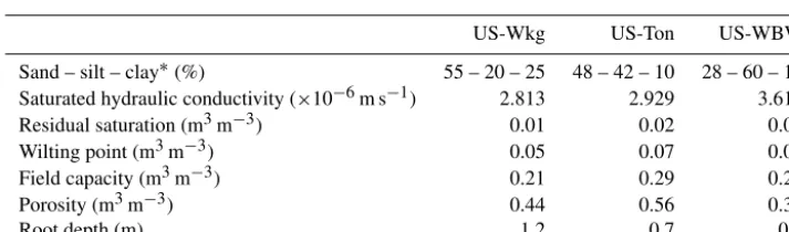
Table 2.Soil and vegetation properties at each study site.
US-Wkg US-Ton US-WBW
Sand – silt – clay∗(%) 55 – 20 – 25 48 – 42 – 10 28 – 60 – 12 Saturated hydraulic conductivity (×10−6m s−1) 2.813 2.929 3.615 Residual saturation (m3m−3) 0.01 0.02 0.05 Wilting point (m3m−3) 0.05 0.07 0.07 Field capacity (m3m−3) 0.21 0.29 0.26 Porosity (m3m−3) 0.44 0.56 0.38
Root depth (m) 1.2 0.7 0.6
∗US-Wkg: Nearing et al. (2005). US-Ton: BADM from the AmeriFlux database. US-WBW: Miller et al. (2007).
the porous medium such as pumping or injection (m3s−1), and Sw is the subsurface water saturation (m3m−3). The MEP-Es model requires soil moisture information to com-pute three parameters: the soil thermal inertia (Is; Eq. 3) and the surface specific humidity of the soil (qss; Eq. 9) and leaf (qls; Eq. 11) surfaces. At the beginning of a given time step, HGS supplies the soil moisture information from the previ-ous time step to the MEP-Emodel, which then computes the evaporation and transpiration rates (Fig. 2). The transpiration and evaporation rates computed with the MEP-Emodel are then transferred to HGS and taken as sinks for the porous medium (0exin Eq. 19). HGS removes water from the soil reservoir based on the root and evaporation depth profiles, which both follow a cubic decay distribution between the sur-face and the maximum root or evaporation depth. At the end of the given time step, HGS calculates the saturation through-out the soil column. Given that the MEP-Es model was not very sensitive to changes in soil thermal inertia, this parame-ter was set as a constant equal to the dry soil thermal inertia (as detailed in the next section) and was not involved in the coupling procedure.
4 Model implementation 4.1 HGS-MEP
The coupled HGS-MEP model was not calibrated in the present study. The soil and vegetation properties were
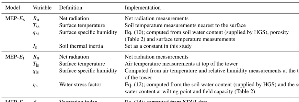
[image:6.612.120.477.237.342.2]rela-Table 3.Implementation of the MEP model of total terrestrial evaporation in this study.
Model Variable Definition Implementation
MEP-Es Rn Net radiation Net radiation measurements
Tss Surface temperature Soil temperature measurements nearest to the surface
qss Surface specific humidity Eq. (10); computed from soil water content (supplied by HGS), porosity (Table 2) and surface temperature measurements
Is Soil thermal inertia Set as a constant in this study
MEP-Et Rn Net radiation Net radiation measurements
Tls Surface temperature Air temperature measurements at top of the tower
qls Surface specific humidity Computed from air temperature and relative humidity measurements at the top of the tower
ηs Water stress factor Eq. (12); computed from the soil water content (supplied by HGS) and the soil water content at wilting point and field capacity (Table 2)
MEP-E fveg Vegetation index Eq. (14); computed from NDVI data
tively robust to variations in saturated hydraulic conductivity and vertical root distribution (Maheu et al., 2018).
Table 3 provides a summary of the implementation of the MEP model of terrestrial evaporation in HGS. In the MEP model of evaporation, skin temperature measurements would ideally be used to set the soil surface temperature (Tss), but since those measurements were not available, we instead used soil temperature measurements nearest to the surface, which is at a depth of 5 cm at US-Wkg, 2 cm at US-Ton and 2 cm at US-WBW. The height above ground (zin Eq. 4) was set to the flux tower height, which was 6.4 m at US-Wkg, 23 m at US-Ton and 36.9 m at US-WBW. At US-Wkg, the dry soil thermal inertia (Idsin Eq. 3) was computed according to Wang et al. (2010) as the regression coefficient between diurnal variations in the ground heat flux and surface tem-perature (830 J m−2K−1s−1/2). Because these data were un-available at US-Ton and US-WBW and given that the model showed little sensitivity to the soil thermal inertia, the dry soil thermal inertia was set equal to 800 J m−2K−1s−1/2for these two sites. In the MEP model of transpiration, the leaf surface temperature was assumed to be equal to the air tem-perature measured above the canopy. Since no measurements of the leaf surface specific humidity were available, we used the specific humidity of the air as a proxy and calculated it from air temperature and relative humidity measurements us-ing the Clausius–Clapeyron equation. To combine the MEP models of evaporation and transpiration (Eq. 13), we com-puted the vegetation index (Eq. 14) using the AVHRR 7 d composite NDVI (https://lta.cr.usgs.gov/NDVI, last access: 4 November 2016). NDVI time series are notoriously noisy because of varying atmospheric conditions and sensor view-ing angles (Hird and McDermid, 2009), and we therefore smoothed the time series by applying a 60 d moving average. Based on Montandon and Small (2008), the NDVI signal for bare soil (NDVI0) was set to 0.2, and the NDVI signal for full vegetation cover varied according to the land cover, with
NDVI∞=0.61 for grassland, NDVI∞=0.69 for woody sa-vanna and NDVI∞=0.85 for deciduous broadleaf forest. 4.1.1 HGS with Penman–Monteith (HGS-PM)
We compared HGS-MEP to simulations of terrestrial evap-oration and soil water content performed with the stand-alone HGS model, in which the Kristensen and Jensen (1975) model is implemented, as described in Sect. 3.2. We used the same soil and root properties defined for the HGS-MEP simulations (Table 2), and the only difference was the terres-trial evaporation model. In HGS, transpiration and evapora-tion are set to occur simultaneously. However, this approach led to a large overestimation of terrestrial evaporation. In the present study, we modified the implementation of the model, and evaporation took place only whenf1(LAI)=0. As for the HGS-MEP model implementation, interception was not considered andEcwas set to zero. The maximum and mini-mum evaporation limiting saturation (Eq. 18) were set to 0.1 (θe1=0.1θs) and 0.5 (θe2=0.5θs; Verbist et al., 2012). Po-tential evaporation (Ep), which is terrestrial evaporation from a saturated land surface, was computed with the Penman– Monteith equation, a physically based model where, simi-lar to the MEP model, the predicted terrestrial evaporation is constrained by available energy at the surface:
Ep= 1 λ
1 (Rn−G)+
ρacp(es−ea)
ra
1+γ1+rs
ra
, (20)
[image:7.612.55.540.84.250.2]US-WBW=100 s m−1 in Kumar et al., 2011), and the canopy aerodynamic resistance (rac) was computed as (Thom, 1975) rac=
1 κ2u
ln
z−d0
z0m
ln
z−d0
z0v
, (21)
where u is the wind speed (m s−1), z is the wind speed measurement height (m), d0 is the zero-plane displacement height (m),z0mis the roughness height for momentum
trans-fer (m) and z0v is the roughness height for water vapour
transfer (m). Equation (21) was derived for neutral atmo-spheric conditions but has also been successfully used to model terrestrial evaporation over a wide range of conditions (Ershadi et al., 2014). Roughness heights were estimated as a fraction of the vegetation height,h(m; Brutsaert, 1982):
d0=0.66h, (22)
z0m=0.1h, (23)
z0v=0.1z0m. (24)
When f1(LAI)=0, the surface resistance (rs) was set to 999 s m−1, the value associated with a barren or sparsely veg-etated land cover in the Noah lookup table (Kumar et al., 2011), and the substrate aerodynamic resistance (ras) was computed as (Shuttleworth and Wallace, 1985)
ras= 1 κ2u
ln
z
z0 0
ln
d 0+z0m
z0 0
, (25)
wherez00is the roughness length of the soil (m), which was set to 0.01 m (Shuttleworth and Wallace, 1985).
Thef1(LAI)function used to describe temporal changes in vegetation (Eq. 16) was computed by rescaling, between 0 and 1, the vegetation indexfveg, an input to the HGS-MEP model.
4.2 Model setup
As a proof of concept, we set up the coupled HGS-MEP and HGS-PM models to perform one-dimensional soil col-umn simulations to evaluate the capability of both models to simulate water fluxes (terrestrial evaporation) and storage (soil moisture). We represented the soil column with a fine (1 cm) vertical resolution and set the soil column depth to ei-ther 1 or 1.5 m in order to capture the entire root zone at each site. We assigned uniform soil properties throughout the soil column, since there were no available data to describe the vertical distribution of soil material with depth. Simulations spanned 5 years at Wkg and Ton and 2.5 years at US-WBW given that data were not available for a longer period. We used soil water content measurement available at differ-ent depths to set initial subsurface conditions, and we used linear interpolation to assign initial conditions at depths with-out measurements. As for initial surface water conditions, we assumed an initial surface water depth of zero given that the soil was not fully saturated. For boundary conditions, we
supplied the model with gap-filled (REddyProc; Reichstein et al., 2005) measurements of precipitation, net radiation, air temperature, relative humidity and soil temperature at a 30 min time step. At the surface, we applied a critical depth boundary condition that allows water to leave the model do-main via overland flow. At the bottom of the soil column, we applied a free drainage boundary condition.
4.3 Model performance
We evaluated the performance of models using a series of metrics comparing observed and simulated values of terres-trial evaporation and soil water content at the three sites. First, we computed the root-mean-square error (RMSE) to assess the mean difference between observed and simulated values. Second, we computed the Nash–Sutcliffe efficiency (NSE), where a value of 1 indicates a perfect agreement be-tween the model and observations and a negative value in-dicates that the average value of observations offers a better predictor than the model. The RMSE and NSE are not inde-pendent metrics of performance given that the NSE is a stan-dardized measure of the mean square error. Still, we chose to report the two commonly used metrics, as they provide an assessment of performance in absolute (RMSE) and rela-tive (NSE) terms. Third, we computed the normalized bench-mark efficiency (BE), which is analogue to the NSE but com-pares the model output to a simple benchmark model, in this case being the interannual mean value for every calendar day (Schaefli and Gupta, 2007). Fourth, we computed the coeffi-cient of determination (R2) that describes the proportion of the total variance in observations explained by the model. Fi-nally, we computed the percent bias (PBIAS) to assess the average tendency of simulated values to be larger (positive bias) or smaller (negative bias) than observations. Equations of performance metrics are listed in Table S1 in the Supple-ment.
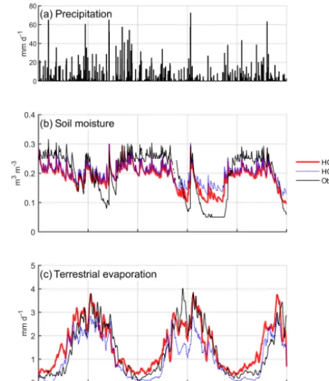
Figure 3. (a)Precipitation as well as observed and modelled(b)daily mean soil water content at a depth of 15 cm, and(c)10 d moving average of terrestrial evaporation at US-Wkg (climate: semi-arid; vegetation: grassland).
5 Results
5.1 Model performance under a semi-arid climate (US-Wkg)
During the study period (2010–2014), the mean annual pre-cipitation at US-Wkg varied between 264 and 415 mm, with 2013 and 2014 being the driest and wettest years, respec-tively (Fig. 3a). Between January and June, pre-monsoon precipitation was relatively low (≤35 mm), with the ex-ception of 2010, which saw 110 mm of rain in the first 6 months of the year. Precipitation was concentrated dur-ing the monsoon periods, and, with the exception of 2010, nearly 80 % occurred between July and September. Figure 3b shows that the HGS-MEP model provided a realistic simula-tion of soil moisture at 15 cm depth (RMSE=0.04 m3m−3; NSE=0.30; Table 4) and was able to capture the sharp rise in soil moisture at the start of the monsoon period in July – note that soil moisture observations were missing between 5 May 2010 and 31 December 2011. Overall, soil moisture at 15 cm depth was generally overestimated (PBIAS=19 %; Table 4) with HGS-MEP, particularly for the lower values outside the monsoon period. For example, the observed an-nual minimum in soil water content was 0.06 m3m−3
be-tween 2012 and 2014, while modelled soil moisture did not fall below 0.12 m3m−3. A similar overestimation was also observed for the upper (z=5 cm) and lower (z=30 cm) soil layers (Fig. S1 in the Supplement).
[image:9.612.104.494.67.384.2]dur-Table 4.Performance of the HGS-MEP and HGS with Penman–Monteith (HGS-PM) models when simulating(a)daily mean soil water content (SWC) at a 15 or 20 cm depth and(b) daily mean total terrestrial evaporation (E) as represented by the root-mean-square error (RMSE), Nash–Sutcliffe efficiency (NSE), benchmark efficiency (BE), coefficient of determination (R2) and percentage bias (PBIAS).
RMSE NSE BE R2 PBIAS
HGS-MEP HGS-PM HGS-MEP HGS-PM HGS-MEP HGS-PM HGS-MEP HGS-PM HGS-MEP HGS-PM
(a)SWC (m3m−3) (%)
US-Wkg 0.04 0.05 0.30 −0.10 −0.35 −1.13 0.62 0.54 19 27
US-Ton 0.03 0.04 0.92 0.88 0.60 0.46 0.94 0.89 −5 0
US-WBW 0.05 0.05 0.61 0.51 −0.22 −0.54 0.74 0.66 −6 −1
(b)E (mm d−1) (%)
US-Wkg 0.31 0.58 0.88 0.57 0.48 −0.86 0.89 0.65 −10 −14
US-Ton 0.43 0.55 0.73 0.56 0.11 −0.45 0.77 0.70 −14 −25
[image:10.612.50.546.106.239.2]US-WBW 0.71 0.74 0.65 0.62 −1.70 −1.93 0.68 0.69 11 −23
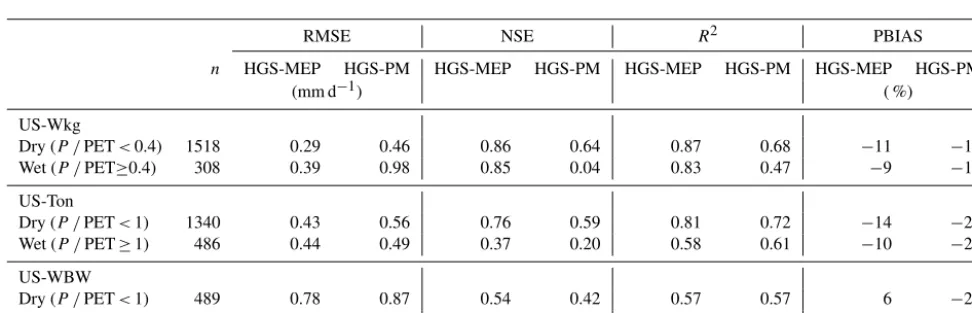
Table 5.Performance of the HGS-MEP and HGS with Penman–Monteith (HGS-PM) models when simulating daily mean total terrestrial evaporation (E) during dry and wet periods, as represented by the root-mean-square error (RMSE), Nash–Sutcliffe efficiency (NSE), coeffi-cient of determination (R2) and percentage bias (PBIAS).nrepresents the number of days.
RMSE NSE R2 PBIAS
n HGS-MEP HGS-PM HGS-MEP HGS-PM HGS-MEP HGS-PM HGS-MEP HGS-PM
(mm d−1) ( %)
US-Wkg
Dry (P /PET<0.4) 1518 0.29 0.46 0.86 0.64 0.87 0.68 −11 −15
Wet (P /PET≥0.4) 308 0.39 0.98 0.85 0.04 0.83 0.47 −9 −12
US-Ton
Dry (P /PET<1) 1340 0.43 0.56 0.76 0.59 0.81 0.72 −14 −24
Wet (P /PET≥1) 486 0.44 0.49 0.37 0.20 0.58 0.61 −10 −27
US-WBW
Dry (P /PET<1) 489 0.78 0.87 0.54 0.42 0.57 0.57 6 −23
Wet (P /PET≥1) 425 0.61 0.54 0.57 0.66 0.65 0.71 26 −24
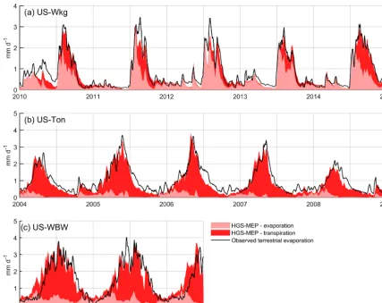
ing which it represented 69 % of the terrestrial evaporation simulated by HGS-MEP (Fig. 4a). During the monsoon pe-riod when vegetation activity is concentrated (July–October), evaporation decreased in importance and, on average, ac-counted for 60 % of the total terrestrial evaporation simulated by HGS-MEP, while transpiration represented 40 % of total terrestrial evaporation. These proportions varied from year to year. For example, 2014 was the wettest year during the study period, and modelled transpiration represented 46 % of total terrestrial evaporation during the monsoon period.
In contrast, modelled transpiration represented 28 % of total terrestrial evaporation during the monsoon period in 2012, although terrestrial evaporation was overall under-estimated by the HGS-MEP model that year. Overall, the HGS-MEP model outperformed the HGS-PM model for the simulation of daily terrestrial evaporation and soil moisture (Fig. 3b). Indeed, performance metrics at the daily timescale show a large decline in the performance of HGS-PM dur-ing wet periods (NSE=0.04) compared with dry periods (NSE=0.64; Table 5). In contrast, the performance of
[image:10.612.55.541.296.452.2]terres-Figure 4. 10 d moving average of observed terrestrial evaporation and modelled terrestrial evaporation partitioned as transpiration and evaporation at(a)US-Wkg (climate: semi-arid; vegetation: grassland),(b)US-Ton (climate: Mediterranean; vegetation: woody savanna) and
[image:11.612.84.511.84.423.2](c)US-WBW (climate: temperate; vegetation: deciduous broadleaf forest).
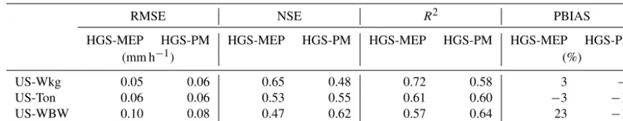
[image:11.612.77.524.514.669.2]Table 6.Performance of the HGS-MEP and HGS with Penman–Monteith (HGS-PM) models when simulating half-hourly mean total terres-trial evaporation, as represented by the root-mean-square error (RMSE), Nash–Sutcliffe efficiency (NSE), coefficient of determination (R2) and percentage bias (PBIAS).
RMSE NSE R2 PBIAS
HGS-MEP HGS-PM HGS-MEP HGS-PM HGS-MEP HGS-PM HGS-MEP HGS-PM
(mm h−1) (%)
US-Wkg 0.05 0.06 0.65 0.48 0.72 0.58 3 −9 US-Ton 0.06 0.06 0.53 0.55 0.61 0.60 −3 −18 US-WBW 0.10 0.08 0.47 0.62 0.57 0.64 23 −18
trial evaporation, as shown by the four performance metrics (RMSE, NSE,R2and PBIAS; Table 6).
5.2 Model performance under a Mediterranean climate (US-Ton)
During the study period (2004–2008), mean annual precip-itation at US-Ton ranged between 371 and 782 mm, with most precipitation concentrated during winter months, from October to May (Fig. 6a). The first two winters (2004– 2005 and 2005–2006) of the study period were particularly wet (precipitation is 717 and 882 mm), while the follow-ing years experienced near-normal precipitation (385 and 392 mm). As shown in Fig. 6b, the HGS-MEP model sim-ulated soil moisture exceptionally well at a 20 cm depth (RMSE=0.03 m3m−3; NSE=0.92; Table 4) and was able to reproduce the decrease in soil moisture as precipitation stops in summer (Fig. 6b). During the wet winter months, the HGS-MEP model slightly underestimated soil mois-ture (PBIAS= −5 %) but still captured the increase in soil moisture during this period. Near the surface (z=0 cm; Fig. S2a), soil moisture was generally underestimated by HGS-MEP during the dry summer months: observed soil water content slowly decreased until it generally reached a minimum of 0.04–0.05 m3m−3at the end of the season, while modelled soil moisture dropped rapidly to reach a minimum value (0.03 m3m−3) close to the residual water content (0.02 m3m−3; Table 2). For the deeper soil layers (z=50 cm), the HGS-MEP model generally overestimated soil moisture during dry summer months, with a modelled minimum of 0.17 m3m−3 compared to an observed mini-mum of 0.14 m3m−3(Fig. S2c).
When simulating terrestrial evaporation, the HGS-MEP model performed well (RMSE=0.43 mm d−1; NSE=0.73), although terrestrial evaporation was underes-timated (PBIAS= −14 %; Table 4). The HGS-MEP model performed particularly well for winter months and was able to capture the increase in terrestrial evaporation from about 0.4 mm d−1(modelled average terrestrial evaporation in September) to 3.3 mm d−1 (modelled average annual maximum terrestrial evaporation) as water became more available. However, following those winter months, as
Figure 6. (a)Precipitation as well as observed and modelled(b)daily mean soil water content at a depth of 20 cm, and(c)10 d moving average of terrestrial evaporation at US-Ton (climate: Mediterranean; vegetation: woody savanna).
5.3 Model performance under a temperate climate (US-WBW)
In the simulation period, 2004 was a relatively wet year (annual precipitation=1600 mm), while 2005 was relatively dry (annual precipitation=995 mm; Fig. 7a). In Fig. 7b, the HGS-MEP model provided a realistic simulation of soil moisture (RMSE=0.05 m3m−3; NSE=0.61; Table 4) and captured the decrease in soil moisture associated with in-creased vegetation activity during the summer. However, soil moisture at a 20 cm depth was generally overestimated by HGS-MEP during the summer, and modelled soil water content did not fall below 0.1 m3m−3, while the observed soil water content reached an annual minimum of 0.08 and 0.05 m3m−3in 2004 and 2005. In contrast, soil moisture dur-ing the winter was generally underestimated by HGS-MEP, with a modelled average soil water content of 0.21 m3m−3 between January and April in comparison with an observed average of 0.26 m3m−3. Overall, a similar pattern (overes-timation of soil moisture in the summer and underestima-tion in the winter) was observed in soil moisture simulaunderestima-tions near the surface (z=5 cm; Fig. S3a). As for deeper soil lay-ers (z=60 cm), soil moisture was systematically
underesti-mated, although this could be due to changes in soil proper-ties given that there is an upper shift in observed soil moisture values compared with upper soil layers (Fig. S3c).
[image:13.612.102.492.68.383.2]mod-elled evaporation dropped to less than 0.1 mm d−1. Tran-spiration simulated by HGS-MEP accounted on average for 57 % of total terrestrial evaporation between October and April, but this proportion increased considerably dur-ing the summer. Indeed, between May and September, mod-elled transpiration represented on average 87 % of total ter-restrial evaporation. Overall, the HGS-MEP model outper-formed HGS-PM, although, as shown by negative BE val-ues, both models had less explanatory power than a sim-ple benchmark model that captures seasonality. The two models performed similarly during dry and wet periods, with only a slight decline in performance at HGS-PM dur-ing dry periods in the summer (NSE=0.42) compared with wet periods in the winter (NSE=0.66; Table 5). Dur-ing summer months, the HGS-PM largely underestimated terrestrial evaporation (PBIAS= −23 %), particularly dur-ing the dry 2005 year (Fig. 7c). As a result, soil mois-ture was overestimated by HGS-PM much more so than with HGS-MEP (Fig. 7b). During winter months, soil mois-ture was generally underestimated, although a similar pat-tern was observed for HGS-MEP. At the diurnal scale, the HGS-PM (NSE=0.62) performed better than HGS-MEP (NSE=0.47) when simulating half-hourly terrestrial evapo-ration, although both models had an important bias, which was positive for HGS-MEP (PBIAS=23 %) and negative for HGS-PM (PBIAS= −18 %; Table 6). This bias is par-ticularly reflected in the simulation of the daily maximum, which was overestimated by HGS-MEP and largely under-estimated by HGS-PM (Fig. 5c). Indeed, the daily maxi-mum observed mid-day at US-WBW is 0.18 mm h−1, while it reached 0.22 mm h−1 with HGS-MEP and 0.13 mm h−1 with HGS-PM.
6 Discussion
6.1 Performance of the HGS-MEP model 6.1.1 HGS-MEP vs. HGS-PM
At the daily timescale, the HGS-MEP model outperformed HGS-PM when simulating terrestrial evaporation at the three study sites, which translated into improved performance for soil moisture modelling as well (Table 4). Notably, we ob-served a weak performance of HGS-PM during wet periods at US-Wkg (P /PET≥0.4) and US-Ton (P /PET≥1; Ta-ble 5). At US-Wkg, this meant that HGS-PM failed to cap-ture the annual maximum terrestrial evaporation, which has important implications for the water budget. In contrast, the weaker performance at US-Ton by HGS-PM, and to a lesser degree by HGS-MEP, meant that the two models struggle to describe the minimum rates of terrestrial evaporation. At US-WBW, both models had a comparable performance, with consistent results for HGS-MEP for wet (P /PET≥1) and
Figure 7. (a) Precipitation as well as observed and modelled
(b)daily mean soil water content at a depth of 20 cm, and(c)10 d moving average of terrestrial evaporation at US-WBW (climate: temperate; vegetation: deciduous broadleaf forest).
dry periods, while HGS-PM performed better during wet pe-riods than dry pepe-riods (Table 5).
[image:14.612.308.545.66.340.2](NSE=0.30, BE= −0.35; Table 4). However, in the absence of parameter calibration, we consider this performance to be more than acceptable given the challenges of modelling wa-ter fluxes under arid climates. Soil moisture was generally overestimated by HGS-MEP during dry periods (Fig. 3), and further work on the definition of the wilting point in arid cli-mates could help improve the performance of the model. In-deed, wilting can occur at a lower threshold than−1.5 MPa (−4 to−2 MPa; Baldocchi et al., 2004) for vegetation having evolved under an arid climate.
At the Mediterranean site US-Ton, daily terrestrial evapo-ration was underestimated by HGS-MEP (PBIAS= −14 %; Table 4), particularly during the second half of the year, as re-duced water supply led to a decline in terrestrial evaporation (Fig. 5). While the HGS-MEP model simulates soil moisture very well at a depth of 20 cm (Fig. 6), it tended to underesti-mate soil moisture close to the surface (Fig. S2a), where the largest proportion of roots is found according to the vertical root distribution defined by HGS (cubic decay distribution between the surface and the maximum root depth). Given that the water stress factor (ηs) is computed from the weighted av-erage soil water content over the root zone (Eq. 12), this un-derestimation of soil moisture near the surface translated into an overestimation of the reduction in transpiration resulting from water stress. We also investigated if the issue of water stress overestimation could be due to a mis-definition of the maximum rooting depth, as trees under a Mediterranean cli-mate have been found to access water from deep soil layers or groundwater (Miller et al., 2010). However, we also simu-lated terrestrial evaporation with the stand-alone MEP model using soil moisture observations, thus avoiding the overesti-mation of water stress near the surface, and instead found a large overestimation of terrestrial evaporation (Fig. S4). These results suggest that increasing the rooting depth to in-crease access to water resources would likely not improve the simulation of terrestrial evaporation. Instead, uncertainty relative to the definition of the vertical root distribution (as opposed to the maximum rooting depth) or, as previously discussed, with the definition of water stress points (wilting point and field capacity) may explain the challenge of simu-lating terrestrial evaporation under water-limited conditions at US-Ton.
At the half-hourly timescale, both MEP and HGS-PM showed lower performance than at a daily timescale when simulating terrestrial evaporation. For example, the NSE varied between 0.56 and 0.88 at a daily timescale (Ta-ble 4), while it varied between 0.47 and 0.65 at a half-hourly timescale (Table 6). At a half-hourly timescale, no model is distinctly superior to another: HGS-MEP performed better at US-Wkg, HGS-PM performed better at US-WBW and both models performed similarly at US-Ton (Table 6). Still, we observed a distinct pattern where peak terrestrial evaporation during the day was generally overestimated by HGS-MEP and underestimated by HGS-PM (Fig. 5). A known issue of energy imbalance, particularly at subdaily timescales, is
as-sociated with eddy covariance measurements (Leuning et al., 2012). This issue typically leads to an underestimation in ob-servations of terrestrial evaporation and could in part explain the apparent issue of overestimation of peak values by HGS-MEP. On the other hand, the negative bias of HGS-PM at the half-hourly timescale (−18 %≤PBIAS≤ −9 %; Table 6) may actually be even more important when taking the energy imbalance issue into account.
Overall, the predictive ability of the MEP model is partic-ularly noteworthy given that we did not rely on calibration and instead used a priori estimation of parameters describ-ing the soil and vegetation. The MEP model thus offers a promising alternative to model hydrologic fluxes without re-lying on calibration (Wagener, 2007). We chose the Penman– Monteith model as a benchmark against which to compare the MEP model, as it is a physically based model that al-lows for a detailed parameterization of vegetation. How-ever, studies have shown that the Penman–Monteith model leads to an underestimation of terrestrial evaporation under a contemporary climate (Ershadi et al., 2014) and an over-estimation under climate change (Milly and Dunne, 2016). Other models could have been considered, although Hajji et al. (2018) demonstrated the superior performance of the MEP model compared with other models such as the modi-fied Priestley–Taylor Jet Propulsion Laboratory (PT-JPL) and the air-relative-humidity-based two-source model (ARTS). 6.1.2 HGS-MEP vs. HGS using observed terrestrial
evaporation as a forcing
overesti-mation bias (19 %; Table 4) than the HGS simulation (10 %; Table 4 in Maheu et al., 2018), which could be due to the underestimation of peak (2011 and 2012) or pre-monsoon (2010, 2012 and 2013) terrestrial evaporation (Fig. 3). At the temperate site (US-WBW), simulations with HGS-MEP and HGS in Maheu et al. (2018) both showed the same pattern of underestimation of soil moisture in the winter and overes-timation in the summer. This suggests that these biases are in good part associated with the definition of soil (hydraulic parameters) or vegetation (root distribution) properties rather than with the MEP model itself.
6.1.3 Partitioning of total terrestrial evaporation by HGS-MEP
In the present study, evaporation simulated by HGS-MEP represented on average 60 % of total terrestrial evaporation at the semi-arid site (US-Wkg) during the monsoon period (Fig. 4a). These results are in line with experimental results from Moran et al. (2009), who estimated that, following the Lehmann lovegrass invasion, evaporation accounted for 55 % of the total terrestrial evaporation during the growing season of a year with average precipitation. Results from the present study are also concordant with those of Scott and Bieder-man (2017), who found that, on average, evaporation rep-resented 54 % of growing-season total terrestrial evaporation at US-Wkg between 2004 and 2015. Using overstory and un-derstory flux tower measurements at the Mediterranean site US-Ton, Miller et al. (2010) found that transpiration from trees dominate during the dry summer months and that un-derstory evaporation (i.e. bare soil evaporation and transpi-ration from grasses and forbs) is close to zero. Our results are consistent with these observations, and according to the HGS-MEP simulation, transpiration accounted on average for 94 % of total terrestrial evaporation (Fig. 4b). At the tem-perate site (US-WBW), soil evaporation, as measured by an understory flux tower, accounted for 16 % of total terrestrial evaporation on an annual basis and for generally less than 8 % of total terrestrial evaporation during the growing sea-son (Wilsea-son et al., 2001). In the present study, soil evapora-tion simulated by HGS-MEP amounted to 13 % of total ter-restrial evaporation during the growing season between May and September (Fig. 4c), which agrees with these experimen-tal estimates. Overall, the HGS-MEP model showed a good capability for the partitioning of total terrestrial evaporation under various climates (semi-arid, Mediterranean and tem-perate); this is a conclusion that was also reached for a hu-mid, energy-limited environment (Wang et al., 2017). 6.2 Using the MEP model to integrate the energy
budget in hydrological modelling: strengths and limitations
The MEP model of land surface fluxes offers an effective means to implement coupled water and energy budget
mod-elling for hydrological applications. First, the MEP model of terrestrial evaporation requires six input variables: net ra-diation, soil surface temperature, leaf surface temperature and specific humidity, vegetation index and soil water con-tent, the last of which can be supplied by a hydrological model. Thus, the MEP model eliminates the need for wind speed and surface roughness (input to the Penman model) or for vertical gradients of temperature and humidity (inputs to the aerodynamic method often implemented in land sur-face models). Second, the MEP model ensures, by design, the closure of the energy balance. As such, terrestrial evapo-ration simulated by the MEP model is constrained by avail-able energy, which avoids issues of overestimation associated with the use of temperature-based PET models for hydrolog-ical projection. Third, the MEP model relies on a small set of equations, making it straightforward to implement, with minimal computational needs. Land surface models also of-fer a means of implementing coupled water and energy bud-get modelling, but contrary to the MEP model, these models are generally complex and computationally heavy. Last, the explicit partitioning of total terrestrial evaporation into evap-oration and transpiration is also a strength of the MEP model given that the water feeding these two fluxes is drawn from different pools. Partitioning has particularly important im-plications for terrestrial evaporation modelling under water-limiting conditions (e.g. arid environments; Kurc and Small, 2004) or under changing land cover conditions (Huxman et al., 2005), and the MEP model thus offers a tool for better representing these conditions in hydrological modelling.
the specific humidity at the soil surface (qss) as well as the water stress factor (ηs) from the subsurface storage compo-nent of the conceptual model. Third, in its current form, the HGS-MEP model is still driven by dependent variables. For example, both net radiation and surface temperature are in-puts to the model, although incoming long-wave radiation, a component of net radiation, is largely dependent on air temperature (used as a proxy for surface temperature Tls). Moreover, soil surface temperature (Tss) is an input to the model even though it is a function of the heat fluxes pre-dicted by the model. In the present project, we have focused on the coupling of water fluxes between HGS and MEP, al-though in the future, the two models could also be more closely coupled, since thermal transport modelling is imple-mented within HGS (Brookfield et al., 2009). In addition to soil moisture information, the HGS model could supply in-formation on soil surface temperature to the MEP model and thus eliminate its need as an input variable. For example, Huang and Wang (2016) simulated surface soil temperature and moisture using a force–restore model that relies on the MEP model to simulate the heat budget.
7 Conclusion
Using the MEP model of land surface fluxes, we proposed a simple approach to integrate energy budget modelling in hydrological models in order to improve the simulation of terrestrial evaporation. The MEP model requires six input variables (net radiation, soil surface temperature and specific humidity, leaf surface temperature and specific humidity and vegetation index) and ensures energy budget closure, which imparts a strong physical basis and avoids issues of oversen-sitivity to air temperature associated with certain PET mod-els. We coupled the MEP model to HGS, an integrated sur-face and subsursur-face hydrologic model. Without calibration, the coupled HGS-MEP model performed well in simulating soil water content and terrestrial evaporation at three Amer-iFlux sites with varying climates (semi-arid, Mediterranean and temperate). For both the simulation of daily soil mois-ture and terrestrial evaporation, HGS-MEP outperformed the stand-alone HGS model where, as defined by the Kristensen and Jensen (1975) model, terrestrial evaporation is derived from potential evaporation, which we computed using the Penman–Monteith equation. Overall, results indicate that, through a simple coupling procedure, the MEP model of-fers a physically constrained approach to simulate terrestrial evaporation in hydrological models. This approach may offer a tool for better assessing climate change impacts on water resources, although the predictive ability of the MEP model under environmental change, may it be natural (e.g. wild-fires) or anthropogenic (e.g. land cover change and climate change), still needs to be assessed. This study focused on the simulation of vertical water fluxes, but to use HGS-MEP for flow simulation and projection, lateral fluxes will need
to be considered in further work. Various routing models are available and could be used in conjunction with HGS-MEP to simulate lateral fluxes in a computationally efficient way. Finally, the present study focused on the application of the HGS-MEP model at snow-free sites, and the MEP model has undergone little testing in cold regions, with tests limited to the snow-free period (Wang et al., 2017). An MEP model for snow surfaces (Wang et al., 2014) is available and could also be integrated to hydrological models to allow energy budget modelling throughout the year in northern environments.
Data availability. Data are available upon request from the corre-sponding author. For AmeriFlux data, see Baldocchi (2016), Mey-ers (2016) and Scott (2016).
Supplement. The supplement related to this article is available on-line at: https://doi.org/10.5194/hess-23-3843-2019-supplement.
Author contributions. AM, FA and DN designed the study. AM im-plemented the methodology and wrote the paper. IH provided help with the implementation of the MEP model. RT provided help with the implementation of the HGS model. All authors contributed to the writing and interpretation of results.
Competing interests. The authors declare that they have no conflict of interest.
Acknowledgements. This research was supported by Natural Sci-ences and Engineering Research Council of Canada, Hydro-Québec, Ouranos, and Environment and Climate Change Canada. We thank Jingfeng Wang (Georgia Tech) for his help with the im-plementation of the MEP model. Funding for AmeriFlux data re-sources was provided by the US Department of Energy’s Office of Science. We thank the primary investigators of the AmeriFlux sites that made this research possible by making their data available: Rus-sel Scott (US-Wkg), Dennis Baldocchi (US-Ton) and Tilden Meyers (US-WBW). All data used in this paper are listed in the tables and references.
Financial support. This research has been supported by the Natural Sciences and Engineering Research Council of Canada (grant nos. RDC/477125-14 and RGPIN/04892-2015).
References
Alves, M., Music, B., Nadeau, D. F., and Anctil, F.: Com-paring the Performance of the Maximum Entropy Produc-tion Model With a Land Surface Scheme in Simulating Sur-face Energy Fluxes, J. Geophys. Res.-Atmos., 124, 3279–3300, https://doi.org/10.1029/2018JD029282, 2019.
Andréassian, V., Perrin, C., and Michel, C.: Impact of imper-fect potential evapotranspiration knowledge on the efficiency and parameters of watershed models, J. Hydrol., 286, 19–35, https://doi.org/10.1016/j.jhydrol.2003.09.030, 2004.
Aquanty.: HydroGeoSphere User Manual – release 1.0, Aquanty Inc, Waterloo, Canada, 2013.
Bae, D. H., Jung, I. W., and Lettenmaier, D. P.: Hydrologic un-certainties in climate change from IPCC AR4 GCM simula-tions of the Chungju Basin, Korea, J. Hydrol., 401, 90–105, https://doi.org/10.1016/j.jhydrol.2011.02.012, 2011.
Baldocchi, D.: AmeriFlux US-Ton Tonzi Ranch, AmeriFlux, https://doi.org/10.17190/AMF/1245971, 2016.
Baldocchi, D. D., Falge, E., Gu, L., Olson, R., Hollinger, D., Running, S., Anthoni, P., Bernhofer, Ch., Davis, K., Evans, R., Fuentes, J., Goldstein, A., Katul, G., Law, B., Lee, X., Malhi, Y., Meyers, T., Munger, W., Oechel, W., Paw U, K. T., Pilegaard, K., Schmid, H. P., Valentini, R., Verma, S., Vesala, T., Wilson, K., and Wofsy, S.: FLUXNET?: A new tool to study the tem-poral and spatial variability of ecosystem-scale carbon dioxide, water vapor, and energy flux densities, B. Am. Meteorol. Soc., 82, 2415–2434, 2001.
Baldocchi, D. D., Xu, L., and Kiang, N.: How plant functional-type, weather, seasonal drought, and soil physical proper-ties alter water and energy fluxes of an oak-grass savanna and an annual grassland, Agr. Forest Meteorol., 123, 13–39, https://doi.org/10.1016/j.agrformet.2003.11.006, 2004.
Breshears, D. D., Adams, H. D., Eamus, D., McDowell, N. G., Law, D. J., Will, R. E., Park Williams, A., and Zou, C. B.: The critical amplifying role of increasing atmospheric moisture demand on tree mortality and associated regional die-off, Front. Plant Sci., 4, 266, https://doi.org/10.3389/fpls.2013.00266, 2013.
Brookfield, A. E., Sudicky, E. A., Park, Y.-J., and Conant Jr., B.: Thermal transport modeling in a fully integrated sur-face/subsurface framework, Hydrol. Process., 23, 2150–2164, https://doi.org/10.1002/hyp.7282, 2009.
Brutsaert, W.: Evaporation into the atmosphere: Theory, history and applications, Springer, Dordrecht, 1982.
Dewar, R. C.: Maximum entropy production and the fluc-tuation theorem, J. Phys. A-Math. Gen., 38, L371–L381, https://doi.org/10.1088/0305-4470/38/21/L01, 2005.
Dewar, R. C.: Maximum entropy production as an inference al-gorithm that translates physical assumptions into macroscopic predictions: Don’t shoot the messenger, Entropy, 11, 931–944, https://doi.org/10.3390/e11040931, 2009.
Donohue, R. J., Mcvicar, T. R., and Roderick, M. L.: As-sessing the ability of potential evaporation formula-tions to capture the dynamics in evaporative demand within a changing climate, J. Hydrol., 386, 186–197, https://doi.org/10.1016/j.jhydrol.2010.03.020, 2010.
Ehret, U., Gupta, H. V., Sivapalan, M., Weijs, S. V., Schyman-ski, S. J., Blöschl, G., Gelfan, A. N., Harman, C., Kleidon, A., Bogaard, T. A., Wang, D., Wagener, T., Scherer, U., Zehe, E., Bierkens, M. F. P., Di Baldassarre, G., Parajka, J., van
Beek, L. P. H., van Griensven, A., Westhoff, M. C., and Win-semius, H. C.: Advancing catchment hydrology to deal with pre-dictions under change, Hydrol. Earth Syst. Sci., 18, 649–671, https://doi.org/10.5194/hess-18-649-2014, 2014.
Ekström, M., Jones, P. D., Fowler, H. J., Lenderink, G., Buishand, T. A., and Conway, D.: Regional climate model data used within the SWURVE project – 1: projected changes in seasonal patterns and estimation of PET, Hydrol. Earth Syst. Sci., 11, 1069–1083, https://doi.org/10.5194/hess-11-1069-2007, 2007.
Ershadi, A., McCabe, M. F., Evan, J. P., Chaney, N. W., and Wood, E. F.: Multi-site evaluation of terrestrial evaporation mod-els using FLUXNET data, Agr. Forest Meteorol., 187, 46–61, https://doi.org/10.1016/j.agrformet.2013.11.008, 2014.
Feddes, R. A., Kowalik, P. J., and Zaradny, H.: Simulation of field water use and crop yield, John Wiley and Sons, New York, 1978. Ferguson, I. M., Jefferson, J. L., Maxwell, R. M., and Kollet, S. J.: Effects of root water uptake formulation on simulated water and energy budgets at local and basin scales, Environ. Earth Sci., 75, 316, https://doi.org/10.1007/s12665-015-5041-z, 2016. Ficklin, D. L. and Novick, K. A.: Historic and projected changes in
vapor pressure deficit suggest a continental-scale drying of the United States atmosphere, J. Geophys. Res., 122, 2061–2079, https://doi.org/10.1002/2016JD025855, 2017.
Gaborit, É., Fortin, V., Xu, X., Seglenieks, F., Tolson, B., Fry, L. M., Hunter, T., Anctil, F., and Gronewold, A. D.: A hydrological prediction system based on the SVS land-surface scheme: effi-cient calibration of GEM-Hydro for streamflow simulation over the Lake Ontario basin, Hydrol. Earth Syst. Sci., 21, 4825–4839, https://doi.org/10.5194/hess-21-4825-2017, 2017.
Gibbens, R. and Lenz, J.: Root system of some Chihuhuan Desert plants, J. Arid Environ., 49, 221–263, 2001.
Gutman, G. and Ignatov, A.: The derivation of the green vege-tation fraction from NOAA/AVHRR data for use in numerical weather prediction models, Int. J. Remote Sens., 19, 1533–1543, https://doi.org/10.1080/014311698215333, 1998.
Hajji, I., Nadeau, D. F., Music, B., Anctil, F., and Wang, J.: Appli-cation of the maximum entropy production model of evapotran-spiration over partially vegetated water-limited land surfaces, J. Hydrometeorol., 19, 989–1005, 2018.
Hamon, W.: Computation of direct runoff amounts from storm rain-fall, Int. Assoc. Sci. Hydrol., 63, 52–62, 1963.
Hird, J. N. and McDermid, G. J.: Noise reduction of NDVI time series: An empirical comparison of se-lected techniques, Remote Sens. Environ., 113, 248–258, https://doi.org/10.1016/j.rse.2008.09.003, 2009.
Hobbins, M. T., Dai, A., Roderick, M. L., and Farquhar, G. D.: Re-visiting the parameterization of potential evaporation as a driver of long-term water balance trends, Geophys. Res. Lett., 35, 1–6, https://doi.org/10.1029/2008GL033840, 2008.
Hoerling, M. P., Eischeid, J. K., Quan, X.-W., Diaz, H. F., Webb, R. S., Dole, R. M., and Easterling, D. R.: Is a transition to semiper-manent drought conditions imminent in the U.S. Great Plains?, J. Climate, 25, 8380–8386, https://doi.org/10.1175/JCLI-D-12-00449.1, 2012.
Huang, S.-Y. and Wang, J.: A coupled force-restore model of sur-face temperature and soil moisture using the maximum entropy production model of heat fluxes, J. Geophys. Res.-Atmos., 121, 7528–7547, https://doi.org/10.1002/2015JD024586, 2016. Huxman, T. E., Wilcox, B. P., Breshears, D. D., Scott, R. L., Snyder,
K. A., Small, E. E., Hultine, K., Pockman, W. T., and Jackson, R. B.: Ecohydrological implications of woody plant encroachment, Ecology, 86, 308–319, 2005.
Ichii, K., Wang, W., Hashimoto, H., Yang, F., Votava, P., Michaelis, A. R., and Nemani, R. R.: Refinement of rooting depths us-ing satellite-based evapotranspiration seasonality for ecosystem modeling in California, Agr. Forest Meteorol., 149, 1907–1918, https://doi.org/10.1016/j.agrformet.2009.06.019, 2009.
Isabelle, P.-E., Nadeau, D., Rousseau, A., and Anctil, F.: Wa-ter budget, performance of evapotranspiration formulations, and their impact on hydrological modeling of a small boreal peatland-dominated watershed, Can. J. Earth Sci., 55, 206–220, https://doi.org/10.1139/cjes-2017-0046, 2018.
Jaynes, E. T.: Information theory and statistical mechanics, Phys. Rev., 106, 620–630, https://doi.org/10.1103/PhysRev.106.620, 1957.
Kay, A. L. and Davies, H. N.: Calculating potential evapora-tion from climate model data: A source of uncertainty for hy-drological climate change impacts, J. Hydrol., 358, 221–239, https://doi.org/10.1016/j.jhydrol.2008.06.005, 2008.
Kingston, D. G., Todd, M. C., Taylor, R. G., Thompson, J. R., and Arnell, N. W.: Uncertainty in the estimation of potential evapo-transpiration under climate change, Geophys. Res. Lett., 36, 3–8, https://doi.org/10.1029/2009GL040267, 2009.
Kleidon, A. and Schymanski, S.: Thermodynamics and optimality of the water budget on land: A review, Geophys. Res. Lett., 35, L20404, https://doi.org/10.1029/2008GL035393, 2008. Koch, J., Cornelissen, T., Fang, Z., Bogena, H., Diekkrüger, B.,
Kollet, S., and Stisen, S.: Inter-comparison of three distributed hydrological models with respect to seasonal variability of soil moisture patterns at a small forested catchment, J. Hydrol., 533, 234–249, https://doi.org/10.1016/j.jhydrol.2015.12.002, 2016. Koedyk, L. P. and Kingston, D. G.: Potential
evapotranspira-tion method influence on climate change impacts on river flow: a mid-latitude case study, Hydrol. Res., 951–963, https://doi.org/10.2166/nh.2016.152, 2016.
Kristensen, K. J. and Jensen, S. E.: A model for estimating actual evapotranspiration from potential evapotranspiration, Nord. Hy-drol., 6, 170–188, https://doi.org/10.2166/nh.1975.012, 1957. Kumar, A., Chen, F., Niyogi, D., Alfieri, J. G., Ek, M., and Mitchell,
K.: Evaluation of a photosynthesis-based canopy resistance for-mulation in the Noah land-surface model, Bound.-Lay. Meteo-rol., 138, 263–284, https://doi.org/10.1007/s10546-010-9559-z, 2011.
Kunstmann, H., Jung, G., Wagner, S., and Clottey, H.: In-tegration of atmospheric sciences and hydrology for the development of decision support systems in sustainable water management, Phys. Chem. Earth, 33, 165–174, https://doi.org/10.1016/j.pce.2007.04.010, 2008.
Kurc, S. A. and Small, E. E.: Dynamics of evapotranspiration in semiarid grassland and shrubland ecosystems during the summer monsoon season, central New Mexico, Water Resour. Res., 40, 1–15, https://doi.org/10.1029/2004WR003068, 2004.
Leuning, R., van Gorsel, E., Massman, W. J., and Isaac, P. R.: Reflections on the surface energy im-balance problem, Agr. Forest Meteorol., 156, 65–74, https://doi.org/10.1016/j.agrformet.2011.12.002, 2012.
Livneh, B., Restrepo, P. J., and Lettenmaier, D. P.: Development of a unified land model for prediction of surface hydrology and land–atmosphere interactions, J. Hydrometeorol., 12, 1299– 1320, https://doi.org/10.1175/2011JHM1361.1, 2011.
Lofgren, B. M., Hunter, T. S., and Wilbarger, J.: Effects of using air temperature as a proxy for potential evapotranspiration in climate change scenarios of Great Lakes basin hydrology, J. Great Lakes Res., 37, 744–752, https://doi.org/10.1016/j.jglr.2011.09.006, 2011.
Maheu, A., Anctil, F., Gaborit, E., Fortin, V., Nadeau, D. F., and Therrien, R.: A field evaluation of soil moisture modeling with the Soil, Vegetation, and Snow (SVS) land surface model using evapotranspiration observations as forcing data, J. Hydrol., 558, 532–545, https://doi.org/10.1016/j.jhydrol.2018.01.065, 2018. Maxwell, R. and Miller, N.: Development of a coupled land
sur-face and groundwater model, J. Hydrometeorol., 6, 233–247, https://doi.org/10.1175/JHM422.1, 2005.
Maxwell, R. M., Putti, M., Meyerhoff, S., Delfs, J.-O., Ferguson, I. M., Ivanov, V., Kim, J., Kolditz, O., Kollet, S. J., Kumar, M., Lopez, S., Niu, J., Paniconi, C., Park, Y.-J., Phanikumar, M. S., Shen, C., Sudicky, E. A., and Sulis, M.: Surface-subsurface model intercomparison: a first set of benchmark results to diag-nose integrated hydrology and feedbacks, Water Resour. Res., 50, 1531–1549, https://doi.org/10.1002/2013WR013725, 2014. McAfee, S. A.: Methodological differences in projected
po-tential evapotranspiration, Clim. Change, 120, 915–930, https://doi.org/10.1007/s10584-013-0864-7, 2013.
McKenney, M. S. and Rosenberg, N. J.: Sensitivity of some po-tential evapotranspiration estimation methods to climate change, Agr. Forest Meteorol., 64, 81–110, https://doi.org/10.1016/0168-1923(95)02239-T, 1993.
McMahon, T. A., Peel, M. C., and Karoly, D. J.: Assessment of precipitation and temperature data from CMIP3 global climate models for hydrologic simulation, Hydrol. Earth Syst. Sci., 19, 361–377, https://doi.org/10.5194/hess-19-361-2015, 2015. McVicar, T. R., Van Niel, T. G., Li, L. T., Roderick, M. L.,
Rayner, D. P., Ricciardulli, L., and Donohue, R. J.: Wind speed climatology and trends for Australia, 1975–2006: Cap-turing the stilling phenomenon and comparison with near-surface reanalysis output, Geophys. Res. Lett., 35, 1–6, https://doi.org/10.1029/2008GL035627, 2008.
Meyers, T.: AmeriFlux US-WBW Walker Branch Watershed, AmeriFlux, https://doi.org/10.17190/AMF/1246109, 2016. Miller, G. R., Chen, X., Rubin, Y., Ma, S., and
Baldoc-chi, D. D.: Groundwater uptake by woody vegetation in a semiarid oak savanna, Water Resour. Res., 46, W10503, https://doi.org/10.1029/2009WR008902, 2010.
Miller, G. R., Baldocchi, D. D., Law, B. E., and Mey-ers, T.: An analysis of soil moisture dynamics using multi-year data from a network of micrometeorologi-cal observation sites, Adv. Water Res., 30, 1065–1081, https://doi.org/10.1016/j.advwatres.2006.10.002, 2007. Milly, P. C. D. and Dunne, K. A.: On the hydrologic