https://doi.org/10.5194/hess-21-2881-2017 © Author(s) 2017. This work is distributed under the Creative Commons Attribution 3.0 License.
Global evaluation of runoff from 10 state-of-the-art
hydrological models
Hylke E. Beck1,3, Albert I. J. M. van Dijk2, Ad de Roo3, Emanuel Dutra4,5, Gabriel Fink6, Rene Orth7, and Jaap Schellekens8
1Civil and Environmental Engineering, Princeton University, Princeton, NJ, USA
2Fenner School of Environment & Society, Australian National University (ANU), Canberra, Australia 3European Commission, Joint Research Centre (JRC), Via Enrico Fermi 2749, 21027 Ispra (VA), Italy 4European Centre for Medium-Range Weather Forecasts (ECMWF), Redding, UK
5Instituto Dom Luiz, Faculdade de Ciências, Universidade de Lisboa, 1749-016 Lisbon, Portugal 6Center for Environmental Systems Research (CESR), University of Kassel, Kassel, Germany 7Institute for Atmospheric and Climate Science, ETH Zurich, Zurich, Switzerland
8Inland Water Systems Unit, Deltares, Delft, the Netherlands
Correspondence to:Hylke E. Beck ([email protected])
Received: 13 March 2016 – Discussion started: 20 May 2016
Revised: 6 April 2017 – Accepted: 29 April 2017 – Published: 12 June 2017
Abstract.Observed streamflow data from 966 medium sized catchments (1000–5000 km2) around the globe were used to comprehensively evaluate the daily runoff estimates (1979– 2012) of six global hydrological models (GHMs) and four land surface models (LSMs) produced as part of tier-1 of the eartH2Observe project. The models were all driven by the WATCH Forcing Data ERA-Interim (WFDEI) meteorologi-cal dataset, but used different datasets for non-meteorologic inputs and were run at various spatial and temporal resolu-tions, although all data were re-sampled to a common 0.5◦ spatial and daily temporal resolution. For the evaluation, we used a broad range of performance metrics related to impor-tant aspects of the hydrograph. We found pronounced inter-model performance differences, underscoring the importance of hydrological model uncertainty in addition to climate in-put uncertainty, for example in studies assessing the hydro-logical impacts of climate change. The uncalibrated GHMs were found to perform, on average, better than the uncali-brated LSMs in snow-dominated regions, while the ensemble mean was found to perform only slightly worse than the best (calibrated) model. The inclusion of less-accurate models did not appreciably degrade the ensemble performance. Overall, we argue that more effort should be devoted on calibrating and regionalizing the parameters of macro-scale models. We further found that, despite adjustments using gauge
obser-vations, the WFDEI precipitation data still contain substan-tial biases that propagate into the simulated runoff. The early bias in the spring snowmelt peak exhibited by most models is probably primarily due to the widespread precipitation un-derestimation at high northern latitudes.
1 Introduction
real-ity, they produce highly uncertain estimates even if we would have access to perfect meteorological data (Beven, 1989).
The quantification of these uncertainties using indepen-dent data sources is of critical importance to advance model development, reject deficient model structures and parame-terizations, quantify model credibility, and ultimately bring some order to the plethora of models (Klemeš, 1986; Wa-gener, 2003; Döll et al., 2015; Clark et al., 2015). There have been several collaborative research efforts focusing on the intercomparison and verification of hydrological models. The earliest were coordinated by the World Meteorological Organization (WMO, 1975, 1986, 1992). Other noteworthy initiatives include the Model Parameter Estimation Experi-ment (MOPEX; Duan et al., 2006), the Global Soil Wetness Project (GSWP; Dirmeyer, 2011), the Water Model Inter-comparison Project (WaterMIP; Haddeland et al., 2011), and the Global Energy and Water Exchanges (GEWEX) Land-Flux project (McCabe et al., 2016). These initiatives have led to numerous multi-model evaluation studies focusing on such hydrological variables as runoff (e.g., Gudmundsson et al., 2012a; Zhou et al., 2012), evaporation (e.g., Schlosser and Gao, 2010; Jiménez et al., 2011; Miralles et al., 2015), soil moisture (e.g., Guo et al., 2007; Xia et al., 2014), snow cover (e.g., Slater et al., 2001), and total water storage (Güntner, 2008), among others.
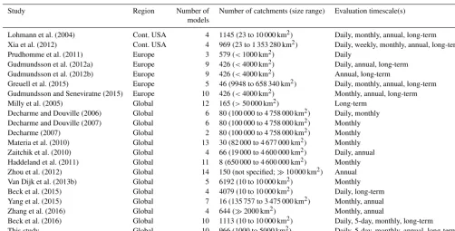
One of the most useful variables for hydrological model evaluation is runoff, since it reflects the integrated response of a host of hydrological processes occurring in a catch-ment (Fekete et al., 2012) and because observations are read-ily available for many catchments across the globe (Hannah et al., 2011). Table 1 lists, to our knowledge, all macro-scale (i.e., continental to global scale) studies evaluating the runoff estimates of multiple models that have been published so far. Out of these 20 studies, two focused on the contermi-nous USA, five focused on Europe, while 13 had a global scope. However, many of these studies used observations from a relatively small number (<100) of large catchments (10 000 km2). The use of a small number of basins limits confidence in the results and precludes a spatially detailed assessment, while the large size of the catchments makes it more difficult to distinguish between deficiencies in the forc-ing, the (sub-)surface component, or the river routing com-ponent of the modeling chain. Moreover, a large number of the studies only evaluated monthly mean runoff, precluding analysis of the shape of individual flow events, or used the Nash and Sutcliffe (1970) efficiency (NSE), which has been criticized in several previous studies for being overly sensi-tive to the timing and magnitude of peak flows (Schaefli and Gupta, 2007; Jain and Sudheer, 2008). Furthermore, many studies considered only a few hydrological models (≤5) or performance metrics (≤2), limiting the insights that can be gained.
As part of tier-1 of the eartH2Observe project, 10 state-of-the-art hydrological models were run globally at a daily time step for the period 1979–2012 using the same forcing dataset,
in an effort to develop a global reanalysis of water resources that supports efficient water management and decision mak-ing (Schellekens et al., 2016). Six of the models are global hydrological models (GHMs) while four of the models are land surface models (LSMs). GHMs have traditionally been designed to simulate (sub-)surface water fluxes and storages, while LSMs have traditionally been designed to simulate the soil–vegetation–atmosphere interactions within climate models (Haddeland et al., 2011; Bierkens, 2015). GHMs gen-erally represent hydrological processes in a more conceptual way, solve only the water balance, commonly operate at daily time steps, and typically have a small number of soil lay-ers (≤3 in the current study) and a single snow layer. Con-versely, LSMs generally represent hydrological processes in a more physically based way, solve both the water and en-ergy balances, typically operate at (sub-)hourly time steps, and tend to have many soil and snow layers (4–11 and 1– 12, respectively, in the current study; for more details on the models, see Table 1 of Schellekens et al., 2016). The present study aims to comprehensively evaluate the runoff estimates of these 10 models across the globe in an effort to answer the following pertinent research questions:
1. How well do the different models simulate runoff? 2. How well do the models perform in terms of long-term
runoff trends?
3. How do the results of the GHMs differ, if at all, from those of the LSMs?
4. Are calibration and regionalization important or even essential?
5. What is the impact of the forcing data on the simulated runoff?
6. How valuable are multi-model ensembles for improving runoff estimates?
Table 1.Overview of, to the best of our knowledge, all macro-scale (continental to global) studies evaluating the runoff estimates of multiple models, sorted by region and then publication date. The present study has been added for the sake of completeness.
Study Region Number of Number of catchments (size range) Evaluation timescale(s) models
Lohmann et al. (2004) Cont. USA 4 1145 (23 to 10 000 km2) Daily, monthly, annual, long-term Xia et al. (2012) Cont. USA 4 969 (23 to 1 353 280 km2) Daily, weekly, monthly, annual, long-term
Prudhomme et al. (2011) Europe 3 579 (<1000 km2) Daily
Gudmundsson et al. (2012a) Europe 9 426 (<4000 km2) Daily, annual, long-term Gudmundsson et al. (2012b) Europe 9 426 (<4000 km2) Annual, long-term
Greuell et al. (2015) Europe 5 46 (9948 to 658 340 km2) Daily, monthly, annual, long-term Gudmundsson and Seneviratne (2015) Europe 10 426 (<4000 km2) Monthly, annual, long-term
Milly et al. (2005) Global 12 165 (>50 000 km2) Long-term
Decharme and Douville (2006) Global 6 80 (100 000 to 4 758 000 km2) Daily, monthly Decharme and Douville (2007) Global 6 80 (100 000 to 4 758 000 km2) Monthly
Decharme (2007) Global 2 80 (100 000 to 4 758 000 km2) Monthly
Materia et al. (2010) Global 13 30 (82 000 to 4 677 000 km2) Monthly Zaitchik et al. (2010) Global 4 66 (19 000 to 4 600 000 km2) Daily, annual Haddeland et al. (2011) Global 11 8 (650 000 to 4 600 000 km2) Monthly Zhou et al. (2012) Global 14 150 (not specified;10 000 km2) Annual Van Dijk et al. (2013b) Global 5 6192 (10 to 10 000 km2) Monthly
Beck et al. (2015) Global 4 4079 (10 to 10 000 km2) Daily, long-term
Yang et al. (2015) Global 7 16 (135 757 to 3 475 000 km2) Monthly, annual
Zhang et al. (2016) Global 4 644 (2000 km2) Monthly, annual
Beck et al. (2016) Global 10 1113 (10 to 10 000 km2) Daily, 5-day, monthly, long-term This study Global 10 966 (1000 to 5000 km2) Daily, 5-day, monthly, annual, long-term
2 Data 2.1 Forcing
The models were all driven by the daily 0.5◦ WATCH Forcing Data ERA-Interim (WFDEI) meteorological dataset (1979–2012; Weedon et al., 2014) with the precipitation (P) data adjusted using the monthly 0.5◦ gauge-based Climate Research Unit (CRU) TS3.1 dataset (Harris et al., 2013). Although the models all used the same P data, they used potential evaporation (PET) derived using diverse formu-lations, ranging from the temperature-based Hamon equa-tion (PCR-GLOBWB) to various radiaequa-tion-based approaches (WaterGAP3, SWBM, and HBV-SIMREG), the Penman– Monteith combination equation (HTESSEL, JULES, LIS-FLOOD, SURFEX, and W3RA), and a surface-energy bal-ance approach (ORCHIDEE). The models also used differ-ent datasets for non-meteorologic inputs. For more details, see Schellekens et al. (2016).
2.2 Simulated runoff
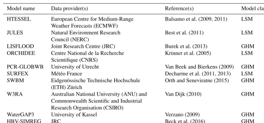
Table 2 lists the 10 state-of-the-art macro-scale hydrologi-cal models of which we evaluated the simulated daily un-routed runoff depths (mm d−1). The data used in this study have been named tier-1 and represent an initial run by all participating modeling groups (Schellekens et al., 2016). All data were acquired through the eartH2Observe Water Cycle Integrator (WCI; http://wci.earth2observe.eu), and for each model the sum of the subsurface and surface runoff
com-ponents was calculated. Six of the models are GHMs (LIS-FLOOD, PCR-GLOBWB, SWBM, W3RA, WaterGAP3, and HBV-SIMREG) and four are LSMs (HTESSEL, JULES, ORCHIDEE, and SURFEX). The GHMs were all run at daily time steps and the LSMs at hourly and 15 min time steps. The models were run at a 0.5◦ spatial resolution, with the exception of LISFLOOD and WaterGAP3, which were run at 0.1◦and 0.08◦, respectively. For the analysis, however, all model output was re-sampled to a common 0.5◦spatial and daily temporal resolution. Four of the models were subjected to varying degrees of calibration to improve their parameters (LISFLOOD, SWBM, WaterGAP3, and HBV-SIMREG; see Sect. 4.4 for specifics). More details concerning the models can be found in Table 1 of Schellekens et al. (2016). 2.3 Observed streamflow
Table 2.Overview of the hydrological models considered in this study. For definitions of the model name acronyms, see Schellekens et al. (2016). Definitions of model-class acronyms: GHM, global hydrological model; and LSM, land surface model.
Model name Data provider(s) Reference(s) Model class
HTESSEL European Centre for Medium-Range Weather Forecasts (ECMWF)
Balsamo et al. (2009, 2011) LSM
JULES Natural Environment Research Council (NERC)
Best et al. (2011) LSM
LISFLOOD Joint Research Centre (JRC) Burek et al. (2013) GHM
ORCHIDEE Centre National de la Recherche Scientifique (CNRS)
Krinner et al. (2005) LSM
PCR-GLOBWB University of Utrecht Van Beek and Bierkens (2009) GHM
SURFEX Météo France Decharme et al. (2011, 2013) LSM
SWBM Eidgenössische Technische Hochschule (ETH) Zürich
Orth and Seneviratne (2015) GHM
W3RA Australian National University (ANU) and Commonwealth Scientific and Industrial Research Organisation (CSIRO)
Van Dijk (2010) GHM
WaterGAP3 University of Kassel Verzano (2009) GHM
HBV-SIMREG JRC Beck et al. (2016) GHM
Table 3.The long-term runoff behavioral signatures considered for evaluating the model performance. The signatures were computed, for
each catchment, from the entire record of simultaneous observed and simulated runoff. Theσvalues represent the spatial variability in the runoff signatures across the landscape.
Runoff Units Description Evaluated flow aspect Standard
signature deviation (σ)
RC − Square-root-transformed runoff coefficient, ratio of long-term runoff toP
Water balance 0.33
MAR pmm yr−1 Square-root-transformed long-term mean annual runoff Water balance 11.21
T50 d The day of the water year marking the timing of the center of mass of flow (Stewart et al., 2005). A water year is defined as the 12-month period from October to September in the Northern Hemisphere and April to March in the Southern Hemisphere
Seasonal flow distribution 34.36
BFI − Base flow index, the ratio of long-term baseflow to total runoff; the baseflow portion of the total runoff was computed following the procedure of Gustard et al. (1992), which takes the minima at 5-day non-overlapping intervals and subsequently connects the valleys in this series of minima to generate baseflow
Partitioning between quickflow and baseflow, flow peakiness
0.18
Q1
√
mm d−1 Square-root-transformed 1st percentile exceedance flow Peak-flow magnitude 1.27
Q99
√
mm d−1 Square-root-transformed 99th percentile exceedance flow Low-flow magnitude 0.21
1. The streamflow record length was required to be ≥ 5 years (not necessarily consecutive) during 1979–2012 (the temporal span of the simulated runoff data). 2. The catchment area had to be <5000 km2, to
mini-mize the effects of channel routing delays and to re-duce the likelihood of significant anthropogenic water use. We could not use larger catchments and evaluate routed streamflow estimates since three of the mod-els did not simulate river routing (JULES, SWBM, and HBV-SIMREG).
3. The catchment area had to be >1000 km2, to pre-vent catchments unrepresentative of the 0.5◦grid cells (2182 km2at 45◦latitude) from confounding the results. 4. To reduce human influences, catchments were required to have<2 % classified as urban (using the “artificial areas” class of the GlobCover version 2.3 map; 300 m resolution; Bontemps et al., 2011) and subject to irri-gation (using version 5 of the Global Map of Irriirri-gation Areas GMIA; 5 min resolution; Siebert et al., 2005). 5. We used the Global Reservoir and Dam (GRanD)
[image:4.612.61.541.353.533.2]reservoir capacity>10 % of the observed mean annual streamflow).
6. Catchments with forest gain or loss>20 % of the catch-ment area (the threshold at which changes in runoff can generally be detected; Bosch and Hewlett, 1982) were excluded using version 1.1 of the Landsat-based forest change dataset (30 m resolution; Hansen et al., 2013). 7. To further reduce the number of disinformative
catch-ments, all streamflow records were visually screened for artifacts and anthropogenic influences (caused by, for example, diversions and impoundments). Further-more, USA catchments flagged as “non-reference” in the GAGES-II database were discarded, and GRDC catchments for which the catchment boundaries could not be reliably determined were discarded (Lehner, 2012).
In total 966 catchments (median size 1970 km2; median record length 19 years during 1979–2012) were found to be suitable for the analysis, of which 641 catchments have daily streamflow data and 325 catchments (mainly located in Russia) have only monthly streamflow data. The locations of the selected catchments will be shown in the Results sec-tion. All observed streamflow data were converted to runoff in mm d−1using the provided catchment areas.
3 Methodology 3.1 Model evaluation
The simulated runoff of the models were evaluated in five ways. First, for each catchment, we calculated the differ-encesD(−) between simulated and observed values of sev-eral runoff signatures. Table 3 lists the six runoff signa-tures selected including their computation from the period with simultaneous simulated and observed runoff. The base-flow index (BFI), square-root-transformed 1st percentile ex-ceedance flow (Q1), and square-root-transformed 99th per-centile exceedance flow (Q99) require daily (rather than monthly) flow data. To compute the flow timing (T50) from monthly data, we first computed daily time series from monthly time series using linear interpolation. Some of the signature values were square-root transformed to give more weight to small values.Dwas computed according to
Dq=
Yqsim−Yqobs
σq
, (1)
where Y represent the values of the runoff signatures (−), the q subscript denotes the runoff signature, and the “sim” and “obs” subscripts refer to simulated and observed, respec-tively. Theσvalues (−) are constants that represent the spa-tial variability in the runoff signatures across the landscape and are used to normalize theDvalues (i.e., to make theD
values of the different signatures intercomparable; see Ta-ble 3). Theσ values were computed by taking the standard deviation of the observed values. Next, the mean D value over all catchments was computed (expressed byD).Dand
Dvalues closer to zero correspond to better model perfor-mance (see Table 4). It should be noted that, althoughD pro-vides a valuable estimate of the overall performance, a good
Dvalue may reflect an overestimation in one region that is compensated by an underestimation in another region.
Second, to evaluate the temporal variability of the simu-lated runoff time series, we computed Pearson linear corre-lation coefficients (r) between daily, log-transformed daily, 5-day, monthly, monthly climatic, and annual time series of simulated and observed runoff (termed rdly, rdly log, r5 day, rmon, rmon clim, andryr, respectively). Therdly, rdly log, and r5 day values were only computed for catchments with daily observations. If monthly data were not supplied by the data providers, monthly values were computed by simple averag-ing of the daily data only if>25 non-missing values were available. Annual values were computed by simple averag-ing of the monthly data (either supplied or computed) only if>10 non-missing values were available. We subsequently computed for each model and metric the meanr value over all catchments, expressed byr. Therandrvalues range from −1 to 1, with higher values corresponding to better model performance (see Table 4).
Third, to summarize the overall performance of each model, we computed for each catchment a summary per-formance statistic (termed OS) incorporating the previously mentioned metrics, and computed the mean value over all catchments (OS). The OS consists of two parts, of which the first (OSsig) considers the performance in terms of runoff sig-natures and is defined as
OSsig= 1−mean
h
|DRC|,|DMAR|,|DT50|,|DBFI|,|DQ1|,|DQ99|
i
. (2)
The second part (OSvar) evaluates the performance in terms of temporal variability, and is defined as
OSvar=mean h
rdly, rdly log, r5 day, rmon, rmon clim, ryr i
. (3)
The summary score is subsequently computed following: OS=OSsig+OSvar
2 . (4)
The BFI, Q1, and Q99 components of Eq. (2) and therdlyand rdly logcomponents of Eq. (3) were omitted if daily observa-tions were unavailable for a particular catchment. Higher OS values correspond to better model performance; the maxi-mum attainable value is 1 (see Table 4).
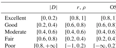
Table 4. Qualitative descriptions of intervals of the performance metrics to aid in interpreting the results.
|D| r,ρ OS
Excellent [0,0.2) [0.8,1] [0.8,1] Good [0.2,0.4) [0.6,0.8) [0.6,0.8) Moderate [0.4,0.6) [0.4,0.6) [0.4,0.6) Fair [0.6,0.8) [0.2,0.4) [0.2,0.4) Poor [0.8,+∞] [−1,0.2) [−∞,0.2)
observed values of the runoff signatures. Spearman rank cor-relation coefficients rather than Pearson linear corcor-relation co-efficients were used to minimize the influence of outliers. The ρ values range from−1 to 1, with higher values cor-responding to better model performance (see Table 4).
Fifth, we computed trends in simulated and observed mean annual runoff time series (termed MAR trend) using the simple non-parametric approach of Sen (1968). We subse-quently calculated the ρ between simulated and observed MAR trends (ρMAR trend), reflecting the agreement in spatial trend patterns.
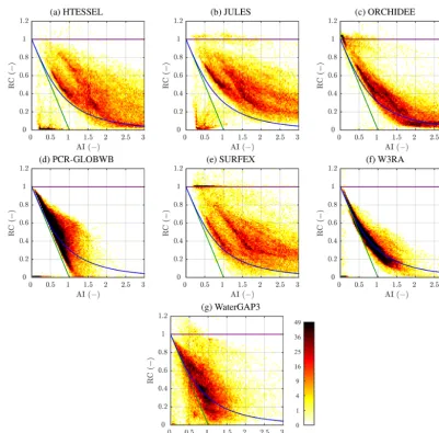
Sixth and last, we produced density plots of grid cell val-ues of aridity index (AI; ratio of long-term available energy toP) versus RC (ratio of long-term simulated runoff toP), revealing how the models behave in terms of RC under differ-ent climatic conditions. To estimate the available energy we used PET for four models (ORCHIDEE, PCR-GLOBWB, W3RA, and WaterGAP3) and net radiation for three mod-els (HTESSEL, JULES, and SURFEX). For the remaining models estimates of the available energy were not available.
For the evaluation, we used for each catchment the simu-lated runoff time series of the 0.5◦ grid cell with its center located within the catchment. However, if multiple grid cell centers were located within the catchment, we calculated the mean simulated runoff time series, and if no grid cell cen-ter was located within the catchment, we used the simulated runoff time series of the grid cell with its center located clos-est to the catchment centroid.
3.2 Multi-model ensembles
Ensemble modeling using the outputs from multiple mod-els or from different realizations of the same model typically improves predictive accuracy and is widely used in atmo-spheric, climate, and hydrological sciences (Wandishin et al., 2001; Tebaldi and Knutti, 2007; Breuer et al., 2009; Viney et al., 2009). We tested two ways of combining the runoff estimates of the individual models into ensembles. First, for each 0.5◦grid cell and day with non-missing values for all models, the mean simulated runoff of the 10 models was calculated (i.e., equal weights were assigned to the models). The resulting runoff estimates will be referred to hereafter as “MEAN-All”. Second, we computed the mean based on only the four models that performed best in terms of OS, to
exam-ine the effect of excluding less-accurate models. These runoff estimates will be referred to hereafter as “MEAN-Best4”. 3.3 Caveats
There are a number of caveats that should be kept in mind when interpreting the results. First, some of the models (no-tably the LSMs) were not traditionally developed to estimate daily runoff for such small catchments. Some of the GHMs, on the other hand, have runoff estimation in small catch-ments among their primary aims (e.g., LISFLOOD, Water-GAP3, W3RA, and HBV-SIMREG), and four GHMs were even explicitly calibrated against observations (LISFLOOD, SWBM, WaterGAP3, and HBV-SIMREG; see Sect. 4.4 for specifics). Second, a model performing poorly in one respect may well perform better for other hydrological variables, cli-mates, catchments, or performance metrics. Third, a poor model performance could simply be the result of subopti-mal parameter values. Fourth, some studies have found that less-accurate models may still lead to a better ensemble mean (Ajami et al., 2006; Viney et al., 2009), although this did not appear to be the case here (see Sect. 4.6). Fifth, we stress that while some models may perform well, they are inherently un-suitable for specific types of impact assessments. For exam-ple, SWBM and HBV-SIMREG do not account for physical differences among land cover types and hence cannot be used for studies assessing the hydrological impacts of changes in land cover. Sixth and finally, the forcing data quality has an important influence on the evaluation results that should not be overlooked.
4 Results and discussion
In this section we will answer the questions posed in the in-troduction.
a much too early bias in the flow timing (T50), SURFEX demonstrated moderate to good performance overall. Simi-lar to SURFEX, W3RA exhibited a very early bias in T50, but generally obtained moderate to good scores. WaterGAP3 and particularly HBV-SIMREG outperformed the other mod-els in most cases. JULES, ORCHIDEE, SURFEX, Water-GAP3, and especially SWBM displayed negativeD values for the BFI and the square-root-transformed 99th flow per-centile (Q99), and a positive D value for the square-root-transformed 1st flow percentile (Q1; Table 5), suggesting they consistently overestimate quickflow. Conversely, LIS-FLOOD and particularly PCR-GLOBWB exhibited positive
D values for BFI and Q99, and a negativeDvalue for Q1, indicating they tend to underestimate quickflow.
Table 5 also presents, for the 10 models and the ensembles, the spatial correlation between simulated and observed val-ues of the runoff signatures (ρ). HTESSEL, JULES, W3RA, WaterGAP3, and HBV-SIMREG performed good overall, while the remaining models performed moderately over-all. PCR-GLOBWB, SURFEX, and WaterGAP3 performed poorly in terms of BFI, while SWBM obtained a poor score for Q99. WaterGAP3 performed good to excellent for all signatures except BFI, likely due to the empirical estima-tion of groundwater recharge and thus baseflow as a func-tion of landscape characteristics (Döll and Fiedler, 2008). HBV-SIMREG attained good to excellent ρ values for all signatures. The models generally performed best for T50 and worst for BFI among the signatures.
Table 5 also shows, for the 10 models and the ensembles, OS scores for the major Köppen–Geiger climate types. We used the newly produced Köppen–Geiger climate map from Beck et al. (2016), which is based on the high-quality World-Clim climatic dataset (Hijmans et al., 2005) supplemented with regional climatic datasets for the USA (Daly et al., 1994) and New Zealand (Tait et al., 2006). All four LSMs (HTESSEL, JULES, ORCHIDEE, and SURFEX) gener-ally demonstrated fair performance in cold and polar cli-mates. Conversely, PCR-GLOBWB demonstrated poor per-formance in tropical and arid climates, likely due to the over-estimation of baseflow. SWBM performed moderately only in arid catchments, probably at least partly due to the lack of baseflow under these conditions (Pilgrim et al., 1988; Beck et al., 2013). Similarly, Orth et al. (2015) found that SWBM performs well during dry periods for eight small Swiss catch-ments (60–392 km2). Only LISFLOOD, WaterGAP3, and HBV-SIMREG exhibited at least moderate performance for all climates.
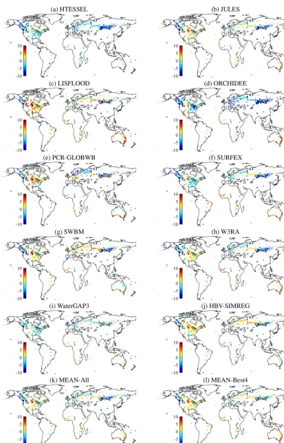
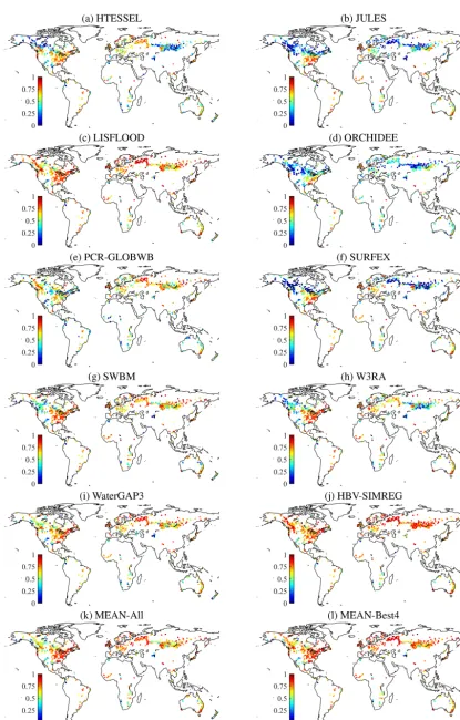
Figure 1 presents, for the 10 models and the ensembles, maps of simulated minus observed MAR for the catchments, revealing the data underlying the MARDandρvalues listed in Table 5. Maps of all other runoff signatures are presented in Supplement Figs. S1.2–1.8. HTESSEL and ORCHIDEE strongly underestimate runoff for most of the catchments, while LISFLOOD appears to strongly overestimate runoff for most of the globe with the exception of snow-dominated
regions. All models showed negative MAR biases in snow-dominated regions such as Alaska, the Rocky Mountains, and southern Russia, while they consistently showed posi-tive MAR biases for the Great Plains (USA) and southern Australia. Figure 2 shows, for the 10 models and the en-sembles, maps of the correlation between simulated and ob-served monthly flows (rmon) for the catchments, showing the data underlying the rmon values presented in Table 5. Maps of all other temporal variability metrics are presented in Figs. S1.9–1.14. In general, the GHMs obtained goodrmon values for most catchments, while the LSMs obtained moder-atermonvalues for most catchments. All LSMs showed poor to fairrmonvalues for snow-dominated catchments.
Although the NSE has been widely criticized for being overly sensitive to the magnitude and timing of peak flows (e.g., Schaefli and Gupta, 2007; Jain and Sudheer, 2008; Criss and Winston, 2008; Gupta et al., 2009), we did cal-culate NSE scores to allow the present results to be put in the context of previous macro-scale studies (see Supplement Ta-ble S1). For most models negative median NSE scores were obtained, similar to Zhang et al. (2016), who evaluated the monthly and annual runoff estimates from 14 (uncalibrated) macro-scale models in 644 large Australian catchments (>
2000 km2). Our scores are, however, slightly lower than those obtained by Lohmann et al. (2004) and Xia et al. (2012), who evaluated the daily runoff estimates from four (uncal-ibrated) macro-scale models in about a thousand small-to-medium sized USA catchments (<10 000 km2), but this is probably attributable to the high quality of the USA forc-ing data (Wu et al., 2017). They are also somewhat lower than those obtained by Decharme and Douville (2007), who evaluated two (uncalibrated) macro-scale models in 80 large catchments (>100 000 km2) around the globe, but this can be explained by their much larger catchment sizes.
in theP, PET, or streamflow data. For the other models this could be indicative of issues with the runoff and/or evapo-ration routines. The larger spread found for the models for which we used net radiation to estimate the available energy (HTESSEL, JULES, and SURFEX; Fig. 3a, b, and e, respec-tively) is because the majority of the net radiation is con-verted to sensible heat rather than latent heat in cold climates (Kleidon et al., 2014).
It is generally difficult to gain insight into why a particular model performs as it does due to the large number of inter-acting model components, equations, and parameters. Never-theless, the underestimation of runoff by HTESSEL probably reflects the excessive evaporation by HTESSEL previously reported by Haddeland et al. (2011). PCR-GLOBWB most likely suffers from suboptimal baseflow-related parameter values, since its structure is similar to that of LISFLOOD, which performs markedly better. SWBM clearly suffers from the absence of a baseflow routine outside (semi-)arid re-gions. Although W3RA and HBV-SIMREG use an identical snow routine, W3RA performs considerably worse in snow-dominated regions, probably because HBV-SIMREG uses a snowfall gauge undercatch correction factor. The unsat-isfactory performance demonstrated by the LSMs in snow-dominated regions could be related to deficiencies in the snow routines or the energy balance estimates (see Sect. 4.3). WaterGAP3 and particularly HBV-SIMREG performed quite well overall, likely because of their comprehensive calibra-tion (see Sect. 4.4). In any case, the pronounced inter-model performance spread found here suggests that model choice should be regarded as a critical step in any hydrological mod-eling study. Moreover, it underscores the importance of hy-drological model uncertainty in addition to climate input un-certainty, as also emphasized in several other recent macro-scale studies (Haddeland et al., 2011; Schewe et al., 2013; Prudhomme et al., 2014; Mendoza et al., 2015b; Giuntoli et al., 2015a). Currently, the large majority of studies as-sessing the hydrological impacts of climate change com-pletely neglect hydrological model uncertainty (Teutschbein and Seibert, 2010).
4.2 How well do the models perform in terms of long-term runoff trends?
The models displayed very similar MAR trends (Fig. S1.8), meaning they respond similarly to climate variability, given that none of the models account for land use or land cover changes, urbanization, reservoir construction, or increasing atmospheric CO2. However, the models obtained rather low spatial (Spearman) correlation coefficients (ρMAR trend) rang-ing from 0.32 (SURFEX) to 0.42 (LISFLOOD; Table 5), in-dicating that the simulated MAR trends correspond fairly to moderately well to the observed ones. These values are lower than the (Pearson) correlation coefficients ranging from 0.52 to 0.63 obtained by Stahl et al. (2012), who evaluated MAR trends from seven models using observations from 293 small
European catchments (100–1000 km2), presumably due to the better quality of the European meteorological forcing and observed streamflow data. Milly et al. (2005) evaluated MAR trends from a 12-model ensemble using observations from 165 large catchments (> 50 000 km2) around the globe, ob-taining a (Pearson) correlation coefficient of 0.34, which is similar to ours. These low correlations, which were some-what unexpected given the relative ease with which MAR can be estimated (e.g., Westerberg and McMillan, 2015; Beck et al., 2015), may be indicative of changes in non-climatic drivers of hydrological change or drift errors in the forcing or observed streamflow data. We expect the inter-model vari-ability in trends to be higher and the agreement with obser-vations to be even lower for seasonal and monthly averages as well as runoff signatures sensitive to the shape of individ-ual flow events (cf. Bastola et al., 2011; Gosling et al., 2011). Overall, these results suggest that studies using global-scale datasets to assess the impacts of past climate change on runoff in small-to-medium-sized catchments should be inter-preted with considerable caution.
4.3 How do the results of the GHMs differ, if at all, from those of the LSMs?
Figure 3.Density plots of grid cell values of aridity index (AI) versus runoff coefficient (RC), for the seven models with data on the available energy. The green line represents the energy limit for which actual evaporation equals PET, the purple line represents the water limit for which runoff equalsP, whereas the blue line represents the Budyko (1974) curve.
(>2000 km2, upper limit not reported) around the globe. The poorer performance obtained by the LSMs is probably in-dicative of differences between the snow routines used by GHMs and LSMs. The GHMs use relatively simple concep-tual temperature-index snow routines driven by air tempera-ture, which can be estimated with relative ease, whereas the LSMs use more complex physically based energy balance snow routines driven by estimates of energy balance compo-nents, which are subject to considerable uncertainty, particu-larly in regions with complex topography (Ferguson, 1999). Although several previous studies have found that the two types of snow routines yield comparable performance (e.g., WMO, 1986; Franz et al., 2008; Zeinivand and De Smedt, 2009; Debele et al., 2010), these studies used a very small number of relatively well-instrumented catchments (six, two, one, and three, respectively), which may have led to
less-generalizable conclusions. Overall, it appears that the energy balance estimates and snow routines used by the LSMs re-quire re-evaluation (cf. Zhang et al., 2016).
4.4 Are calibration and regionalization important or even essential?
2011; Minville et al., 2014). Yet, despite the development of numerous calibration techniques over the last 50 years (Dawdy and O’Donnell, 1965; Duan et al., 2004) and the current widespread availability of streamflow observations (Hannah et al., 2011), macro-scale models generally tend to be uncalibrated (Sooda and Smakhtin, 2015; Bierkens, 2015; Kauffeldt et al., 2016). This is perhaps mainly due to (i) the substantial amount of work involved with calibra-tion (e.g., Bock et al., 2015), (ii) the risk of obtaining un-realistic parameters due to equifinality and data issues (An-dréassian et al., 2012), and (iii) the lack of a commonly ac-cepted regionalization technique (Beck et al., 2016). In ad-dition, the modeler may feel that since their model is phys-ically based, it does not require calibration (Beven, 1989). LSMs in particular are rarely calibrated against runoff, likely because (i) runoff estimation is generally not among the pri-mary aims of LSMs; (ii) for water transport in the soil, LSMs typically use Richards–Darcy type equations, which are com-putationally expensive and require a fine vertical and tempo-ral soil discretization; and (iii) LSMs often do not account for river routing, confounding the calibration of large catch-ments. Instead, the parameters in macro-scale models are usually based on “expert opinion” and thus founded on the bold assumption that the modeler sufficiently understands the hydrological processes, feedbacks, and parameter inter-actions taking place within the model for any location on Earth.
Nevertheless, out of the 10 models considered in this study, four use parameters derived by calibration (LISFLOOD, SWBM, WaterGAP3, and HBV-SIMREG all GHMs). LISFLOOD was calibrated against ob-served streamflow for 24 large catchments (84 230 to 4 680 000 km2) across the globe using the WFDEI forcing and an aggregate objective function incorporating bias, NSE, and log-transformed NSE computed from daily streamflow data. The calibration might have influenced the present eval-uation; although we used much smaller catchments (1000 to 5000 km2), 47 % of our catchments are located within the calibration catchments. SWBM uses a spatially uniform pa-rameter set based on calibration using the E-OBS forcing (Haylock et al., 2008) against European data on such key hy-drologic variables as soil moisture, total water storage, evap-oration, and runoff (Orth and Seneviratne, 2015). For the calibration against runoff, they used observations from 436 small European catchments (mostly<1000 km2), and con-sidered daily and monthly correlations as well as bias. The calibrated parameter set was subsequently applied globally. Besides the addition of a baseflow routine, SWBM would probably benefit from regionalized parameters that vary ac-cording to landscape characteristics. WaterGAP3 has been calibrated using the WFDEI forcing in terms of bias for the interstation regions (the catchment of a station excluding the catchments of nested upstream stations) of 2071 stations (catchment size ranging from 2830 to 966 321 km2) around the globe, some of which have also been used in the current
evaluation. The calibrated parameters were subsequently re-gionalized to ungauged regions using multiple linear regres-sion based on six predictors (Döll et al., 2003). The model does indeed perform very well for MAR and thus RC, but this did not necessarily translate into good performance for BFI (Table 5, and Figs. 1 and 2). HBV-SIMREG also uses regionalized parameter fields, produced by transferring cali-brated parameters from 674 small-to-medium sized “donor” catchments (10 to 10 000 km2) across the globe to “receptor” grid cells with similar climatic and physiographic character-istics (Beck et al., 2016). In their study, Beck et al. (2016) show that HBV using spatially uniform parameters performs within the range of the other models, confirming that the relatively good performance of HBV-SIMREG stems from the regionalization exercise. In addition, although Beck et al. (2016) did not use the WFDEI forcing for the calibration, they calibrated against several of the performance metrics also used here and used 179 of our catchments as parameter donors, further explaining the relatively good performance obtained by HBV-SIMREG (Table 5, and Figs. 1 and 2).
Overall, it appears that the calibration exercises for Wa-terGAP3, HBV-SIMREG, and possibly LISFLOOD have re-sulted in markedly improved performance. However, Water-GAP3 performed poorly in terms ofρBFI(Table 5), meaning the calibration of MAR did not translate into better BFI per-formance. These results underscore the benefits of calibrated parameters over a priori parameters (cf. Duan et al., 2006; Hunger and Döll, 2008; Nasonova et al., 2009; Rosero et al., 2011; Greuell et al., 2015; Zhang et al., 2016) and highlight the importance of using an objective function for the cali-bration that incorporates a broad range of metrics related to various important aspects of the hydrograph (cf. Gupta et al., 2008; Vis et al., 2015; Shafii and Tolson, 2015). These results also emphasize the usefulness of regionalization techniques (Parajka et al., 2013), which typically enhance performance over the entire model domain and are thus of particular value for macro-scale modeling, given that the majority of the land surface is ungauged or poorly gauged (Sivapalan, 2003; Han-nah et al., 2011). However, although there are numerous stud-ies performing regionalization at a regional scale (see re-views by He et al., 2011; Hrachowitz et al., 2013; Razavi and Coulibaly, 2013; Parajka et al., 2013), only a few studies have attempted regionalization at a macro-scale (see review by Beck et al., 2016). We argue that more effort should be de-voted to regionalizing the parameters of macro-scale models (cf. Bierkens, 2015; Döll et al., 2015).
4.5 What is the impact of the forcing data on the simulated runoff?
There are not only strong inter-model differences in the per-formance patterns but also clear inter-model similarities, sug-gesting that the forcing data quality imparts a strong limit on the performance. This is most notable for the MAR met-ric: all models showed negative biases in MAR in snow-dominated regions such as Alaska, the Rocky Mountains, and southern Russia, while they consistently showed positive bi-ases in MAR for the Great Plains (USA) and southern Aus-tralia (Fig. 1). The high spatial correlation in the performance patterns suggests that these consistent performance patterns may be due to biases in the WFDEIP data, rather than bi-ases in the streamflow observations, which are unlikely to be spatially correlated.
It is conceivable that biases are present in the WFDEIP
data, because (i) the monthly CRU dataset, which has been used to correct the WFDEI dataset, is based on only a subset of the available gauges and does not explicitly account for orographic effects; (ii) in sparsely gauged regions the cor-rection using CRU is more likely to deteriorate rather than improve theP estimates; and (iii) the Adam and Lettenmaier (2003) gauge undercatch correction factors are based on in-terpolation of a very sparse sample of gauges and thus sub-ject to considerable uncertainty. For the conterminous USA we quantified the biases in the WFDEI P data using the high-quality Parameter-elevation Relationships on Indepen-dent Slopes Model (PRISM) climatic dataset (Daly et al., 1994), which is based on considerably more gauges than CRU and includes sophisticated corrections for orography. Figure 4a shows the bias in mean annual P from WFDEI relative to that from PRISM, suggesting that the WFDEIP
data are indeed subject to large biases. Figure 4b shows the bias in MAR from the MEAN-All ensemble relative to MAR from the observations, revealing a comparable bias pattern, thus confirming that the biases in the WFDEIP propagate in the simulated runoff. The correlation coefficient between the MAR andP bias values is 0.58, indicating a moderately strong relationship. These P biases appear to translate into even more pronounced runoff biases in (semi-)arid regions (notably the northern Great Plains; Fig. 4b and c) due to the highly nonlinear response behavior in these environments (Lidén and Harlin, 2000; Fekete et al., 2004; Van Dijk et al., 2013a). We were unable to quantify the P biases globally since no other independent, global-scaleP dataset exists (the WorldClim and CHPclim datasets are likely to exhibit simi-lar biases as the CRU TS3.1 dataset, given that they are based on similar sets of gauges). However, we expect theP biases to be at least similar, if not more severe, outside the well-instrumented conterminous USA (cf. Fekete et al., 2004; Hi-jmans et al., 2005; Biemans et al., 2009; Zhou et al., 2012; Kauffeldt et al., 2013; Greuell et al., 2015). It should be noted that biases in PET are probably of secondary importance as
compared with biases inP (Donohue et al., 2010; Sperna Weiland et al., 2011; Seiller and Anctil, 2015).
The global-scale quantification and reduction of theseP
biases should be a priority for future research. Satellite-derived P offers unique opportunities in this regard (e.g., Funk et al., 2015) that extend beyond the tropics with the re-cent launch of the Global Precipitation Measurement (GPM) mission (Smith et al., 2007). Another little-explored way of reducingP uncertainty is by “doing hydrology backwards”; that is, to use information on other hydrological variables, for example, satellite-derived surface soil moisture (e.g., Brocca et al., 2014), streamflow observations (e.g., Adam et al., 2006; Beck et al., 2017), and snow-depth observations (e.g., Cherry et al., 2005) to reconstructP through hydrological modeling. Arguably the most important obstacles to combin-ing multiple data sources are the inconsistent temporal cov-erage and scale of different data sources and the general lack of error/uncertainty estimates.
Although the models all used the sameP data, they used different formulations to compute PET, which has likely con-tributed to differences in simulated runoff among the models in energy-limited regions (Weiß and Menzel, 2008; Kingston et al., 2009; Haddeland et al., 2011; Weedon et al., 2011; Sperna Weiland et al., 2011). However, PET data were avail-able for only four models, which is insufficient to examine whether the PET formulation has had a discernible influence on the simulated runoff, given the numerous other differences in structure and parameterization among the models. 4.6 How valuable are multi-model ensembles?
The multi-model ensemble MEAN-All incorporated all 10 models, while MEAN-Best4 incorporated only LISFLOOD, W3RA, WaterGAP3, and HBV-SIMREG (i.e., the four mod-els that performed best in terms of OS; Table 5). MEAN-All and MEAN-Best4 were found to perform better than all indi-vidual models (with the exception of HBV-SIMREG, which has been comprehensively calibrated; Table 5, and Figs. 1 and 2). These results highlight the benefits of multi-model ensembles, in line with several previous studies (Ajami et al., 2006; Duan et al., 2007; Viney et al., 2009; Materia et al., 2010; Velázquez et al., 2010; Gudmundsson et al., 2012a; Xia et al., 2012; Yang et al., 2015). The similar OS scores obtained by MEAN-All and MEAN-Best4 (0.57 and 0.60, respectively; Table 5) suggests that the inclusion of less-accurate models has only limited adverse effects. It may be worthwhile for future studies to examine the benefits of more sophisticated multi-model combination techniques involving bias correction or model weighting (e.g., Ajami et al., 2006; Duan et al., 2007; Bohn et al., 2010). These weights can sub-sequently be transferred from gauged to ungauged areas us-ing regionalization techniques typically used for hydrologi-cal model parameters (Blöschl et al., 2013).
Figure 4.For the conterminous USA,(a)the bias in mean annualP from WFDEI relative to PRISM,(b)the bias in MAR from the MEAN-All ensemble relative to the observations, and(c)the aridity index, the ratio of mean annual PET (computed from PRISM air temperature using Hargreaves et al., 1985) toP (PRISM; note the nonlinear color scale). Each data point in(b)represents a catchment centroid. The bias in(a)and(b)was computed followingB=(X−R)/(X+R), whereBis the bias,Xthe uncertain value, andRthe reference value. Bvalues range from−1 to 1. A 100 % overestimation results inB=1/3, whereas a 50 % underestimation results inB= −1/3.
means the model was run multiple (10) times globally using different (regionalized) parameter sets representing differ-ent catchmdiffer-ent response behaviors (Beck et al., 2016). HBV-SIMREG obtained slightly better performance than both MEAN-All and MEAN-Best4 overall (Table 5), tentatively suggesting that a multi-parameterization ensemble for a sin-gle, sufficiently flexible model provides performance com-parable to a multi-model ensemble (cf. Oudin et al., 2006; Yang et al., 2011; Coxon et al., 2014). If this is confirmed, it would negate the need to set up, run, and maintain mul-tiple models, and incentivize the development of a single community hydrological model (cf. Weiler and Beven, 2015) as well as modeling systems allowing for the selection of alternative model structures (cf. Bierkens, 2015), such as the Framework for Understanding Structural Errors (FUSE; Clark et al., 2008), Noah Multi-Parameterization (Noah-MP; Niu et al., 2011), and SUPERFLEX (Fenicia et al., 2011). 4.7 Do all models show the early bias in runoff timing
in snow-dominated catchments previously documented and what is the cause?
With the exception of ORCHIDEE and HBV-SIMREG, all models showed early T50 biases in snow-dominated regions (Fig. S1.3), indicating that the models produce the spring snowmelt peak early, as has also been reported in several previous studies using different models and forcing data (Lohmann et al., 2004; Slater et al., 2007; Decharme and Douville, 2007; Balsamo et al., 2009; Zaitchik et al., 2010; Beck et al., 2015). The early runoff timing is probably
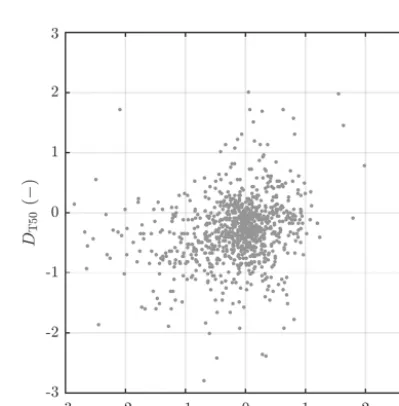
pri-Figure 5.Scatterplot of the difference between simulated
(MEAN-All) and observed-transformed RC (DRC) versus the difference be-tween simulated (MEAN-All) and observed T50 (DT50) for the catchments (n=966).
[image:15.612.327.527.358.561.2]tend to exhibit an early bias in T50 (i.e., negativeDT50) and vice versa. The absence or misrepresentation of certain pro-cesses that delay snowmelt runoff in the models may have exacerbated the early runoff timing problem. Examples of such processes include the isothermal phase change of the snowpack, retainment of meltwater in the snowpack in pore spaces, infiltration of meltwater into the soil, meltwater re-freezing during cold days and nights, and ice jams in rivers. On the whole, more research is needed to ascertain the exact reasons of the early runoff timing.
5 Conclusions
The runoff estimates from 10 state-of-the-art macro-scale hydrological models, all forced with the WFDEI dataset, were evaluated using observations from 966 medium-sized catchments around the globe. With reference to the questions posed in the introduction, the following was found:
1. The performance differed markedly among models, un-derscoring the importance of hydrological model uncer-tainty in addition to climate input unceruncer-tainty, and sug-gesting that model choice should be regarded as a criti-cal step in any hydrologicriti-cal modeling study.
2. The models displayed similar MAR trends, although they were in poor agreement with observed trends. Model-based runoff trends in small-to-medium sized catchments should thus be interpreted with considerable caution.
3. Considering only the uncalibrated models, the GHMs performed similarly to the LSMs in rainfall-dominated regions but consistently better than the LSMs in snow-dominated regions, perhaps due to the use of more data-demanding snow routines or the misrepresentation of frozen soil and snowmelt processes by the LSMs. 4. The models that have been calibrated obtained higher
scores for the performance metrics incorporated in the respective objective functions used for calibration. 5. The WFDEIP forcing data still appear to contain
sub-stantial biases, despite adjustments using gauge obser-vations. ThesePbiases translate into biases in the simu-lated runoff, which are amplified in (semi-)arid regions. In snow-dominated regions there appears to be a consis-tent underestimation inP and thus simulated runoff. 6. The multi-model ensembles obtained only slightly
worse performance than the best (calibrated) model, and the inclusion of less-accurate models did not severely degrade the performance. A multi-parameterization en-semble for a single, sufficiently flexible model is easier to realize but we speculate may yield the same perfor-mance benefits as a multi-model ensemble.
7. Most models were indeed found to generate the spring snowmelt peak early, probably due to the previously mentionedP underestimation and the absence or mis-representation of certain processes that delay snowmelt runoff in the models.
Data availability. All model outputs are available via the eartH2Observe Water Cycle Integrator (WCI; http: //wci.earth2observe.eu).
The Supplement related to this article is available online at https://doi.org/10.5194/hess-21-2881-2017-supplement.
Author contributions. H. B. designed and performed the model evaluation and wrote most of the manuscript. A. v. D., A. d. R., E. D., G. F., R. O., and J. S. helped with the interpretation of the results and contributed to writing of the manuscript. H. B., A. v. D., A. d. R., E. D., G. F., and R. O. assisted in running the hydrological models and making available the model output.
Competing interests. The authors declare that they have no conflict of interest.
Acknowledgements. The Global Runoff Data Centre (GRDC) and the US Geological Survey (USGS) are thanked for providing most of the observed streamflow data. We gratefully acknowledge the modeling groups participating in the eartH2Observe project for providing the simulated runoff data. Lukas Gudmundsson and an anonymous reviewer are thanked for their comments on an earlier draft. This research received funding from the European Union Seventh Framework Programme (FP7/2007–2013) under grant agreement no. 603608, “Global Earth Observation for integrated water resource assessment”: eartH2Observe. The views expressed herein are those of the authors and do not necessarily reflect those of the European Commission.
Edited by: S. Schymanski
Reviewed by: L. Gudmundsson and one anonymous referee
References
Adam, J. C. and Lettenmaier, D. P.: Adjustment of global gridded precipitation for systematic bias, J. Geophys. Res.-Atmos., 108, 4257, https://doi.org/10.1029/2002JD002499, 2003.
Adam, J. C., Clark, E. A., Lettenmaier, D. P., and Wood, E. F.: Cor-rection of global precipitation products for orographic effects, J. Clim., 19, 15–38, https://doi.org/10.1175/JCLI3604.1, 2006. Ajami, N. K., Duan, Q., Gao, X., and Sorooshian, S.: Multimodel
Andréassian, V., Lerat, J., Loumagne, C., Mathevet, T., Michel, C., Oudin, L., and Perrin, C.: What is really undermining hydrologic science today?, Hydrol. Process., 21, 2819–2822, 2007. Andréassian, V., Le Moine, N., Perrin, C., Ramos, M. H., Oudin,
L., Mathevet, T., Lerat, J., and Berthet, L.: All that glitters is not gold: the case of calibrating hydrological models, Hydrol. Process., 26, 2206–2210, 2012.
Balsamo, G., Beljaars, A., Scipal, K., Viterbo, P., van den Hurk, B., Hirschi, M., and Betts, A. K.: A revised hydrology for the ECMWF model: verification from field site to terrestrial water storage and impact in the integrated forecast system, J. Hydrom-eteorol., 10, 623–643, 2009.
Balsamo, G., Pappenberger, F., Dutra, E., Viterbo, P., and van den Hurk, B.: A revised land hydrology in the ECMWF model: a step towards daily water flux prediction in a fully-closed water cycle, Hydrol. Process., 25, 1046–1054, 2011.
Bastola, S., Murphy, C., and Sweeney, J.: The role of hydrological modeling uncertainties in climate change impact assessments of Irish river catchments, Adv. Water Resour., 34, 562–576, 2011. Beck, H. E., van Dijk, A. I. J. M., Miralles, D. G., de Jeu, R. A. M.,
Bruijnzeel, L. A., McVicar, T. R., and Schellekens, J.: Global patterns in baseflow index and recession based on streamflow ob-servations from 3394 catchments, Water Resour. Res., 49, 7843– 7863, 2013.
Beck, H. E., van Dijk, A. I. J. M., and de Roo, A.: Global maps of streamflow characteristics based on observations from several thousand catchments, J. Hydrometeorol., 16, 1478–1501, 2015. Beck, H. E., van Dijk, A. I. J. M., de Roo, A.,
Mi-ralles, D. G., McVicar, T. R., Schellekens, J., and Brui-jnzeel, L. A.: Global-scale regionalization of hydrologic model parameters, Water Resour. Res., 52, 3599–3622, https://doi.org/10.1002/2015WR018247, 2016.
Beck, H. E., van Dijk, A. I. J. M., Levizzani, V., Schellekens, J., Miralles, D. G., Martens, B., and de Roo, A.: MSWEP: 3-hourly 0.25◦global gridded precipitation (1979–2015) by merg-ing gauge, satellite, and reanalysis data, Hydrol. Earth Syst. Sci., 21, 589–615, https://doi.org/10.5194/hess-21-589-2017, 2017. Best, M. J., Pryor, M., Clark, D. B., Rooney, G. G., Essery, R. .
L. H., Ménard, C. B., Edwards, J. M., Hendry, M. A., Porson, A., Gedney, N., Mercado, L. M., Sitch, S., Blyth, E., Boucher, O., Cox, P. M., Grimmond, C. S. B., and Harding, R. J.: The Joint UK Land Environment Simulator (JULES), model description — Part 1: Energy and water fluxes, Geosci. Model Dev., 4, 677– 699, https://doi.org/10.5194/gmd-4-677-2011, 2011.
Beven, K. J.: Changing ideas in hydrology — the case of physically-based models, J. Hydrol., 105, 157–172, 1989.
Biemans, H., Hutjes, R. W. A., Kabat, P., Strengers, B. J., Gerten, D., and Rost, S.: Effects of precipitation uncertainty on discharge calculations for main river basins, J. Hydrometeorol., 10, 1011– 1025, 2009.
Bierkens, M. F. P.: Global hydrology 2015: state, trends, and directions, Water Resour. Res., 51, 4923–4947, https://doi.org/10.1002/2015WR017173, 2015.
Bierkens, M. F. P., Bell, V. A., Burek, P., Chaney, N., Condon, L. E., David, C. H., de Roo, A., Döll, P., Drost, N., Famiglietti, J. S., Flörke, M., Gochis, D. J., Houser, P., Hut, R., Keune, J., Kol-let, S., Maxwell, R. M., Reager, J. T., Samaniego, L., Sudicky, E., Sutanudjaja, E. H., van de Giesen, N., Winsemius, H., and
Wood, E.: Hyper-resolution global hydrological modelling: what is next?, Hydrol. Process., 29, 310–320, 2015.
Blöschl, G. and Sivapalan, M.: Scale issues in hydrological mod-elling: A review, Hydrol. Process., 9, 251–290, 1995.
Blöschl, G., Sivapalan, M., Wagener, T., Viglione, A., and Savenije, H., eds.: Runoff Prediction in Ungauged Basins: synthesis across Processes, Places and Scales, Cambridge University Press, New York, US, 2013.
Bock, A. R., Hay, L. E., McCabe, G. J., Markstrom, S. L., and Atkinson, R. D.: Parameter regionalization of a monthly water balance model for the conterminous United States, Hydrol. Earth Syst. Sci., 20, 2861–2876, https://doi.org/10.5194/hess-20-2861-2016, 2016.
Bohn, T. J., Sonessa, M. Y., and Lettenmaier, D. P.: Seasonal hydro-logic forecasting: do multimodel ensemble averages always yield improvements in forecast skill?, J. Hydrometeorol., 11, 1358– 1372, 2010.
Bontemps, S., Defourny, P., and van Bogaert, E.: GlobCover 2009, products description and validation report, Tech. rep., ESA Glob-Cover project, available at: http://ionia1.esrin.esa.int (last access: June 2016), 2011.
Bosch, J. M. and Hewlett, J. D.: A review of catchment experiments to determine the effect of vegetation changes on water yield and evapotranspiration, J. Hydrol., 55, 3–23, 1982.
Breuer, L., Huisman, J. A., Willems, P., Bormann, H., Bronstert, A., Croke, B. F. W., Frede, H., Gräffe, T., Hubrechts, L., Jakeman, A. J., Kite, G., Lanini, J., Leavesley, G., Lettenmaier, D. P., Lind-ström, G., Seibert, J., Sivapalan, M., and Viney, N. R.: Assessing the impact of land use change on hydrology by ensemble model-ing (LUCHEM). I: Model intercomparison with current land use, Adv. Water Resour., 32, 129–146, 2009.
Brocca, L., Ciabatta, L., Massari, C., Moramarco, T., Hahn, S., Hasenauer, S., Kidd, R., Dorigo, W., Wagner, W., and Levizzani, V.: Soil as a natural rain gauge: estimating global rainfall from satellite soil moisture data, J. Geophys. Res.-Atmos., 119, 5128– 5141, 2014.
Budyko, M. I.: Climate and life, Academic Press, New York, 1974. Burek, P., van der Knijff, J., and de Roo, A.: LISFLOOD Distributed Water Balance and Flood Simulation Model Revised User Man-ual, Tech. Rep. EUR 26162 EN, Joint Research Centre (JRC), Ispra, Italy, https://doi.org/10.2788/24719, 2013.
Cherry, J. E., Tremblay, L. B., Déry, S. J., and Stieglitz, M.: Re-constructing solid precipitation from snow depth measurements and a land surface model, Water Resour. Res., 41, W09401, https://doi.org/10.1029/2005WR003965, 2005.
Clark, M. P., Slater, A. G., Rupp, D. E., Woods, R. A., Vrugt, J. A., Gupta, H. V., Wagener, T., and Hay, L. E.: Framework for Under-standing Structural Errors (FUSE): a modular framework to di-agnose differences between hydrological models, Water Resour. Res., 44, W00B02, https://doi.org/10.1029/2007WR006735, 2008.
Clark, M. P., Fan, Y., Lawrence, D. M., Adam, J. C., Bolster, D., Gochis, D. J., Hooper, R. P., Kumar, M., Leung, L. R., Mackay, D. S., Maxwell, R. M., Shen, C., Swenson, S. C., and Zeng, X.: Improving the representation of hydrologic processes in Earth System Models, Water Resour. Res., 51, 5929–5956, https://doi.org/10.1002/2015WR017096, 2015.
be-havior in a limits-of-acceptability framework for 24 UK catch-ments, Hydrol. Process., 28, 6135–6150, 2014.
Criss, R. E. and Winston, W. E.: Do Nash values have value? Discussion and alternate proposals, Hydrol. Process., 22, 2723– 2725, 2008.
Daly, C., Neilson, R. P., and Phillips, D. L.: A statistical-topographic model for mapping climatological precipitation over mountainous terrain, J. Appl. Meteorol., 33, 140–158, 1994. Dawdy, D. R. and O’Donnell, T.: Mathematical models of
catch-ment behavior, J. Hydr. Eng. Div.-ASCE, 91, 123–137, 1965. Debele, B., Srinivasan, R., and Gosain, A. K.: Comparison of
Process-Based and Temperature-Index Snowmelt Modeling in SWAT, Water Resour. Manag., 24, 1065–1088, 2010.
Decharme, B.: Influence of runoff parameterization on conti-nental hydrology: Comparison between the Noah and the ISBA land surface models, J. Geophys. Res., 112, D19108, https://doi.org/10.1029/2007JD008463, 2007.
Decharme, B. and Douville, H.: Uncertainties in the GSWP-2 pre-cipitation forcing and their impacts on regional and global hy-drological simulations, Clim. Dynam., 27, 695–713, 2006. Decharme, B. and Douville, H.: Global validation of the ISBA
sub-grid hydrology, Clim. Dynam., 29, 21–37, 2007.
Decharme, B., Boone, A., Delire, C., and Noilhan, J.: Lo-cal evaluation of the Interaction between Soil Biosphere At-mosphere soil multilayer diffusion scheme using four pedo-transfer functions, J. Geophys. Res.-Atmos., 116, D20126, https://doi.org/10.1029/2011JD016002, 2011.
Decharme, B., Martin, E., and Faroux, S.: Reconciling soil ther-mal and hydrological lower boundary conditions in land surface models, J. Geophys. Res.-Atmos., 118, 7819–7834, 2013. Dirmeyer, P. A.: A history and review of the Global Soil Wetness
Project (GSWP), J. Hydrometeorol., 12, 729–749, 2011. Döll, P. and Fiedler, K.: Global-scale modeling of
ground-water recharge, Hydrol. Earth Syst. Sci., 12, 863–885, https://doi.org/10.5194/hess-12-863-2008, 2008.
Döll, P., Kaspar, F., and Lehner, B.: A global hydrological model for deriving water availability indicators: model tuning and vali-dation, J. Hydrol., 270, 105–134, 2003.
Döll, P., Douville, H., Güntner, A., Müller Schmied, H., and Wada, Y.: Modelling Freshwater Resources at the global scale: challenges and prospects, Surv. Geophys., 37, 1–26, https://doi.org/10.1007/s10712-015-9343-1, 2015.
Donohue, R. J., McVicar, T. R., and Roderick, M. L.: Assessing the ability of potential evaporation formulations to capture the dynamics in evaporative demand within a changing climate, J. Hydrol., 386, 186–197, 2010.
Duan, Q., Schaake, J., and Koren, V.: A Priori estimation of land surface model parameters, in: Land Surface Hydrology, Meteo-rology, and Climate: Observations and Modeling, edited by: Lak-shmi, V., Albertson, J., and Schaake, J., no. 3 in Water Science and Application, AGU, Washington, DC, US, 77–94, 2001. Duan, Q., Gupta, H. V., Sorooshian, S., Rousseau, A. N., and
Tur-cotte, R.: Calibration of watershed models, vol. Water Science and Application, American Geophysical Union, 2004.
Duan, Q., Schaake, J., Andréassian, V., Franks, S., Goteti, G., Gupta, H. V., Gusev, Y. M., Habets, F., Hall, A., Hay, L., Hogue, T., Huang, M., Leavesley, G., Liang, X., Nasonova, O. N., Noil-han, J., Oudin, L., Sorooshian, S., Wagener, T., and Wood, E. F.: Model Parameter Estimation Experiment (MOPEX): An
overview of science strategy and major results from the second and third workshops, J. Hydrol., 320, 3–17, 2006.
Duan, Q., Ajami, N. K., Gao, X., and Sorooshian, S.: Multi-model ensemble hydrologic prediction using Bayesian model averag-ing, Adv. Water Resour., 30, 1371–1386, 2007.
Falcone, J. A., Carlisle, D. M., Wolock, D. M., and Meador, M. R.: GAGES: A stream gage database for evaluating natural and al-tered flow conditions in the conterminous United States, Ecol-ogy, 91, 621, 2010.
Fekete, B. M., Vörösmarty, C. J., Roads, J. O., and Willmott, C. J.: Uncertainties in precipitation and their impacts on runoff esti-mates, J. Clim., 17, 294–304, 2004.
Fekete, B. M., Looser, U., Pietroniro, A., and Robarts, R. D.: Ratio-nale for monitoring discharge on the ground, J. Hydrometeorol., 13, 1977–1986, 2012.
Fenicia, G., Kavetski, D., and Savenije, H. H. G.: Elements of a flexible approach for conceptual hydrological modeling: 1. Mo-tivation and theoretical development, Water Resour. Res., 47, https://doi.org/10.1029/2010WR010174, 2011.
Ferguson, R. I.: Snowmelt runoff models, Prog. Phys. Geog., 23, 205–227, 1999.
Franz, K. J., Hogue, T. S., and Sorooshian, S.: Operational snow modeling: Addressing the challenges of an energy balance model for National Weather Service forecasts, J. Hydrol., 360, 48–66, 2008.
Freeze, R. A. and Harlan, R. L.: Blueprint for a physically-based, digitally-simulated hydrologic response model, J. Hydrol., 9, 237–258, 1969.
Funk, C., Verdin, A., Michaelsen, J., Peterson, P., Pedreros, D., and Husak, G.: A global satellite assisted precipitation climatology, Earth Syst. Sci. Data, 7, 275–287, https://doi.org/10.5194/essd-7-275-2015, 2015.
Giuntoli, I., Vidal, J., Prudhomme, C., and Hannah, D. M.: Future hydrological extremes: the uncertainty from multiple global cli-mate and global hydrological models, Earth Syst. Dynam., 6, 267–285, 2015a.
Giuntoli, I., Vilarini, G., Prudhomme, C., Mallakpour, I., and Han-nah, D. M.: Evaluation of global impact models’ ability to re-produce runoff characteristics over the central United States, J. Geophys. Rese.-Atmos., 120, 9138–9159, 2015b.
Gosling, S. N., Taylor, R. G., Arnell, N. W., and Todd, M. C.: A comparative analysis of projected impacts of cli-mate change on river runoff from global and catchment-scale hydrological models, Hydrol. Earth Syst. Sci., 15, 279–294, https://doi.org/10.5194/hess-15-279-2011, 2011.
Greuell, W., Andersson, J. C. M., Donnelly, C., Feyen, L., Gerten, D., Ludwig, F., Pisacane, G., Roudier, P., and Schaphoff, S.: Evaluation of five hydrological models across Europe and their suitability for making projections under climate change, Hydrol. Earth Syst. Sci. Discuss., 12, 10289–10330, https://doi.org/10.5194/hessd-12-10289-2015, 2015.
Gudmundsson, L. and Seneviratne, S. I.: Towards observation-based gridded runoff estimates for Europe, Hydrol. Earth Syst. Sci., 19, 2859–2879, https://doi.org/10.5194/hess-19-2859-2015, 2015.
Hydrological Model Simulations to Observed Runoff Percentiles in Europe, J. Hydrometeorol., 13, 604–620, 2012a.
Gudmundsson, L., Wagener, T., Tallaksen, L. M., and Engeland, K.: Evaluation of nine large-scale hydrological models with respect to the seasonal runoff climatology in Europe, Water Resour. Res., 48, W11504, https://doi.org/10.1029/2011WR010911, 2012b. Güntner, A.: Improvement of global hydrological models using
GRACE data, Surv. Geophys., 29, 375–397, 2008.
Guo, Z., Dirmeyer, P. A., Gao, X., and Zhao, M.: Improving the quality of simulated soil moisture with a multi-model ensemble approach, Q. J. R. Meteor. Soc., 133, 731–747, 2007.
Gupta, H. V., Wagener, T., and Liu, Y.: Reconciling theory with observations: elements of a diagnostic approach to model evalu-ation, Hydrol. Process., 22, 3802–3813, 2008.
Gupta, H. V., Kling, H., Yilmaz, K. K., and Martinez, G. F.: Decom-position of the mean squared error and NSE performance criteria: Implications for improving hydrological modelling, J. Hydrol., 370, 80–91, 2009.
Gupta, H. V., Perrin, C., Blöschl, G., Montanari, A., Kumar, R., Clark, M., and Andréassian, V.: Large-sample hydrology: a need to balance depth with breadth, Hydrol. Earth Syst. Sci., 18, 463– 477, https://doi.org/10.5194/hess-18-463-2014, 2014.
Gustard, A., Bullock, A., and Dixon, J. M.: Low flow estimation in the United Kingdom, Tech. Rep. 108, Institute of Hydrology, Wallingford, UK, 1992.
Haddeland, I., Clark, D. B., Franssen, W., F, L., Voß, F., Arnell, N. W., Bertrand, N., Best, M., Folwell, S., Gerten, D., Gomes, S., Gosling, S. N., Hagemann, S., Hanasaki, N., Harding, R., Heinke, J., Kabat, P., Koirala, S., Oki, T., Polcher, J., Stacke, T., Viterbo, P., Weedon, G. P., and Yehm, P.: Multimodel Estimate of the Global Terrestrial Water Balance: Setup and First Results, J. Hydrometeorol., 12, 869–884, 2011.
Hancock, S., Huntley, B., Ellis, R., and Baxter, R.: Biases in Re-analysis Snowfall Found by Comparing the JULES Land Surface Model to GlobSnow, J.Clim., 27, 624–632, 2014.
Hannah, D. M., Demuth, S., Van Lanen, H. A. J., Looser, U., Prud-homme, C., Rees, G., Stahl, K., and Tallaksen, L. M.: Large-scale river flow archives: importance, current status and future needs, Hydrol. Process., 25, 1191–1200, 2011.
Hansen, M. C., Potapov, P. V., Moore, R., Hancher, M., Turubanova, S. A., Tyukavina, A., Thau, D., Stehman, S. V., Goetz, S. J., Loveland, T. R., Kommareddy, A., Egorov, A., Chini, L., Justice, C. O., and Townshend, J. R. G.: High-resolution global maps of 21st-century forest cover change, Science, 342, 850–853, 2013. Hargreaves, G. L., Hargreaves, G. H., and Riley, J. P.: Irrigation
water requirements for Senegal River Basin, J. Irrig. Drain. E.-ASCE, 111, 265–275, 1985.
Harris, I., Jones, P. D., Osborn, T. J., and Lister, D. H.: Updated high-resolution grids of monthly climatic observations – the CRU TS3.10 dataset, Int. J. Climatol., 34, 623–642, 2013. Haylock, M. R., Hofstra, N., Klein Tank, A. M. G., Klok,
E. J., Jones, P., and New, M.: A European daily high-resolution gridded data set of surface temperature and precipi-tation for 1950–2006, J. Geophys. Res.-Atmos., 113, D20119, https://doi.org/10.1029/2008JD010201, 2008.
He, Y., Bárdossy, A., and Zehe, E.: A review of regionalisation for continuous streamflow simulation, Hydrol. Earth Syst. Sci., 15, 3539–3553, https://doi.org/10.5194/hess-15-3539-2011, 2011.
Hijmans, R. J., Cameron, S. E., Parra, J. L., Jones, P. G., and Jarvis, A.: Very high resolution interpolated climate surfaces for global land areas, Int. J. Climatol., 25, 1965–1978, 2005.
Hrachowitz, M., Savenije, H. H. G., Blöschl, G., McDonnell, J. J., Sivapalan, M., Pomeroy, J. W., Arheimer, B., Blume, T., Clark, M. P., Ehret, U., Fenicia, F., Freer, J. E., Gelfan, A., Gupta, H. V., Hughes, D. A., Hut, R. W., Montanari, A., Pande, S., Tetzlaff, D., Troch, P. A., Uhlenbrook, S., Wagener, T., Winsemius, H. C., Woods, R. A., Zehe, E., and Cudennec, C.: A decade of Predic-tions in Ungauged Basins (PUB) – a review, Hydrol. Sci. J., 58, 1198–1255, 2013.
Hunger, M. and Döll, P.: Value of river discharge data for global-scale hydrological modeling, Hydrol. Earth Syst. Sci., 12, 841– 861, https://doi.org/10.5194/hess-12-841-2008, 2008.
Jain, S. K. and Sudheer, K. P.: Fitting of hydrologic models: a close look at the Nash-Sutcliffe index, J. Hydrol. Engin., 13, 981–986, 2008.
Jiménez, C., Prigent, C., Mueller, B., Seneviratne, S. I., Mc-Cabe, M. F., Wood, E. F., Rossow, W. B., Balsamo, G., Betts, A. K., Dirmeyer, P. A., Fisher, J. B., Jung, M., Kanamitsu, M., Reichle, R. H., Reichstein, M., Rodell, M., Sheffield, J., Tu, K., and Wang, K.: Global intercomparison of 12 land surface heat flux estimates, J. Geophys. Res., 116, D02102, https://doi.org/10.1029/2010JD014545, 2011.
Kauffeldt, A., Halldin, S., Rodhe, A., Xu, C.-Y., and West-erberg, I. K.: Disinformative data in large-scale hydrolog-ical modelling, Hydrol. Earth Syst. Sci., 17, 2845–2857, https://doi.org/10.5194/hess-17-2845-2013, 2013.
Kauffeldt, A., Wetterhall, F., Pappenberger, F., Salamon, P., and Thielen, J.: Technical review of large-scale hydrologi-cal models for implementation in operational flood forecasting schemes on continental level, Environ. Modell. Soft., 75, 68–76, https://doi.org/10.1016/j.envsoft.2015.09.009, 2016.
Kingston, D. G., Todd, M. C., Taylor, R. G., Thompson, J. R., and Arnell, N. W.: Uncertainty in the estimation of potential evap-otranspiration under climate change, Geophys. Res. Lett., 36, L20403, https://doi.org/10.1029/2009GL040267, 2009. Kleidon, A., Renner, M., and Porada, P.: Estimates of the
climato-logical land surface energy and water balance derived from maxi-mum convective power, Hydrol. Earth Syst. Sci., 18, 2201–2218, https://doi.org/10.5194/hess-18-2201-2014, 2014.
Klemeš, V.: Operational testing of hydrological simulation models, Hydrol. Sci. J., 31, 13–24, 1986.
Knutti, R.: Should we believe model predictions of future climate change?, Philos. T. R. Soc. Lond. S-A, 366, 4647–4664, 2008. Krinner, G., Viovy, N., de Noblet-Ducoudré, N., Ogée, J., Polcher,
J., Friedlingstein, P., Ciais, P., Sitch, S., and Prentice, I. C.: A dynamic global vegetation model for studies of the cou-pled atmosphere-biosphere system, Global Biogeochem. Cy., 19, GB1015, https://doi.org/10.1029/2003GB002199, 2005. Lehner, B.: Derivation of watershed boundaries for GRDC
gaug-ing stations based on the HydroSHEDS drainage network, Tech. Rep. 41, Global Runoff Data Centre (GRDC), Federal Institute of Hydrology (BfG), Koblenz, Germany, 2012.