www.hydrol-earth-syst-sci.net/21/65/2017/ doi:10.5194/hess-21-65-2017
© Author(s) 2017. CC Attribution 3.0 License.
Event-scale power law recession analysis:
quantifying methodological uncertainty
David N. Dralle1, Nathaniel J. Karst2, Kyriakos Charalampous1,3, Andrew Veenstra1, and Sally E. Thompson1 1University of California Berkeley, Department of Civil and Environmental Engineering, Berkeley, CA, USA 2Babson College, Department of Mathematics, Wellesley, MA, USA
3University of Bristol, Department of Civil Engineering, Bristol, UK
Correspondence to:David N. Dralle ([email protected])
Received: 9 July 2016 – Published in Hydrol. Earth Syst. Sci. Discuss.: 25 August 2016 Revised: 4 December 2016 – Accepted: 8 December 2016 – Published: 4 January 2017
Abstract.The study of single streamflow recession events is receiving increasing attention following the presentation of novel theoretical explanations for the emergence of power law forms of the recession relationship, and drivers of its variability. Individually characterizing streamflow recessions often involves describing the similarities and differences be-tween model parameters fitted to each recession time series. Significant methodological sensitivity has been identified in the fitting and parameterization of models that describe pop-ulations of many recessions, but the dependence of estimated model parameters on methodological choices has not been evaluated for event-by-event forms of analysis. Here, we use daily streamflow data from 16 catchments in northern Cali-fornia and southern Oregon to investigate how combinations of commonly used streamflow recession definitions and fit-ting techniques impact parameter estimates of a widely used power law recession model. Results are relevant to water-sheds that are relatively steep, forested, and rain-dominated. The highly seasonal mediterranean climate of northern Cal-ifornia and southern Oregon ensures study catchments ex-plore a wide range of recession behaviors and wetness states, ideal for a sensitivity analysis. In such catchments, we show the following: (i) methodological decisions, including ones that have received little attention in the literature, can im-pact parameter value estimates and model goodness of fit; (ii) the central tendencies of event-scale recession parameter probability distributions are largely robust to methodological choices, in the sense that differing methods rank catchments similarly according to the medians of these distributions; (iii) recession parameter distributions are method-dependent, but roughly catchment-independent, such that changing the
choices made about a particular method affects a given pa-rameter in similar ways across most catchments; and (iv) the observed correlative relationship between the power-law re-cession scale parameter and catchment antecedent wetness varies depending on recession definition and fitting choices. Considering study results, we recommend a combination of four key methodological decisions to maximize the quality of fitted recession curves, and to minimize bias in the related populations of fitted recession parameters.
1 Introduction
Streamflow recession analysis has the goal of characteriz-ing recession behavior in terms of phenomenological mod-els of decreases in flow (Q, with units of L T−1or L3T−1) over time, typically represented with a power law differential equation (Boussinesq, 1877; Hall, 1968; Tallaksen, 1995): dQ
dt = −aQ
b⇒Q(t )=Q1−b
0 −(1−b)at
1−1b
. (1)
Classical recession seeks a single, effective parameteriza-tion of the power law recession model. With some excep-tions (e.g., Lamb and Beven, 1997; Wittenberg, 1994), these approaches typically perform the fitting step in a single oper-ation:[log(Q), log(−dQ/dt )]point pairs are computed for multiple recession periods, and the recession parameters are then obtained from the slope and intercept of a line fitted to the [log(Q), log(−dQ/dt )] point cloud (e.g., Brutsaert and Nieber, 1977; Stoelzle et al., 2013; Tague and Grant, 2004; Basso et al., 2015; Clark et al., 2009; Kirchner, 2009; Sawaske and Freyberg, 2014; Bogaart et al., 2016). This form of “lumped” recession analysis is empirically and the-oretically motivated. Practically, it reasonably captures ob-served nonlinearity in the hydrograph recession. Theoreti-cally, it uses a model form that is predicted by solutions of the hydraulic groundwater equations (Boussinesq, 1904; Troch et al., 2013). Lumped recession analysis has been used for inverse modeling, the development of flow separation algo-rithms, characterization of aquifer properties, and parameter-ization of hydrologic models, among other applications (Vo-gel and Kroll, 1992; Rupp and Selker, 2006a; Rupp et al., 2004; Szilagyi et al., 1998; Huyck et al., 2005; Bogaart et al., 2016; Tague and Grant, 2004).
Recently, several authors have attributed physical meaning to observed variabilityacrossindividual recessions within a single catchment, triggering an increase in event-scale re-cession analyses (Dralle et al., 2015, 2016; Ghosh et al., 2016; Ye et al., 2014; Wittenberg, 1999; Biswal and Marani, 2010, 2014; Biswal and Nagesh, 2014; Harman et al., 2009; Mutzner et al., 2013; Bart and Hope, 2014; Shaw, 2016; Patnaik et al., 2015; Shaw and Riha, 2012; Vogel and Kroll, 1996; Chen and Krajewski, 2016). Whereas classical, lumped recession analysis seeks a single recession model pa-rameterization to describe all hydrograph recessions for an individual catchment, the goal of event-scale recession anal-ysis is to interpret variations in catchment response to rain-fall as a function of the properties of rainrain-fall events (e.g., Harman et al., 2009) or the catchment state (e.g., Biswal and Marani, 2010; Shaw and Riha, 2012). Motivations for event-scale analysis include testing physical theories that predict variability in power law streamflow recessions (e.g Harman et al., 2009; Biswal and Marani, 2010), detection of human land use impacts on catchment water balance (e.g., Bogaart et al., 2016), and prediction of extent of the wetted channel network (Ghosh et al., 2016; Shaw, 2016).
Among the many issues associated with event-scale anal-ysis (Dralle et al., 2015), perhaps the most challenging are the numerous subjective choices needed to establish consis-tent criteria for recession identification and fitting (Wester-berg and McMillan, 2015). For lumped analyses, Brutsaert and Nieber (1977) established a derivative-based method, which avoids the issue of needing to determine the precise start day of a recession event. Event-scale analyses, however, must identify the start and end of each recession event and select one of many fitting techniques to obtain (a,b) values.
Despite the growing number of event-scale recession stud-ies, it remains unclear to what extent the particular method of recession extraction and fitting could alter features of the computed populations of recession parameters. If uncertainty due to methodological choices exceeds physically derived variations in the recession parameters, new and less ambigu-ous methods will be needed to allow empirical comparative analyses, and to test hypotheses derived from novel theories (e.g., Biswal and Marani, 2010; Clark et al., 2009; Harman et al., 2009). Previous work has demonstrated that method dependent variability in recession parameters in lumped analysis can be larger than natural variability between catch-ments (Stoelzle et al., 2013). For event-scale recession anal-ysis, Chen and Krajewski (2016) demonstrate sensitivity of the recession exponent to recession length and start time rel-ative to a flow peak. However, no systematic study has been undertaken to examine sensitivity of botha andb to some of the most common methodological choices made during event-scale power law recession analysis. Given the early stage of event-scale recession exploration, it is an oppor-tune time to determine the methodological limitations associ-ated with event-scale techniques, hopefully supporting inter-comparability and consistency in future work.
Analogously to Stoelzle et al. (2013) and Chen and Kra-jewski (2016), this study examines the sensitivity of reces-sion parameter values to the various methodological choices to be made when performing event-scale recession extraction and fitting. Specifically, we seek to address four primary re-search questions:
– Research question 1 – how do methodological choices impact fit quality of the power law recession model? – Research question 2 – when catchments are ranked by
fitted recession parameter statistics, is the rank order de-pendent on methodological choices?
– Research question 3 – how do methodological choices affect the empirical frequency distributions (over the pe-riod of record) of recession parameter values?
– Research question 4 – how might methodological choices affect relationships between a given recession parameter and other physical measures of catchment state, such as catchment wetness?
In seeking answers to these questions, we recognize that, unlike lumped recession analysis (Vogel and Kroll, 1992; Brutsaert and Nieber, 1977; Kirchner, 2009), no set of canon-ical methods of event-scale recession analysis have been es-tablished. We propose breaking down the two steps of re-cession analysis – rere-cession extraction and power law model parameterization – into four methodological choices: three concerning recession extraction and one concerning model parameterization:
G
[image:3.612.313.541.66.220.2]age number
Figure 1.Green lines correspond to periods during which stream-flow data were available for each catchment.
our analysis) for a recession period to be selected for analysis. Recessions less than the minimum duration are discarded.
2. The definition of the beginning of a recession event– the start of a recession event is usually determined by a flow peak filtering algorithm applied to the stream-flow time series. Commonly, peaks are identified using a simple flow threshold, wherein flow peaks exceeding the threshold are flagged as potential starts to a reces-sion event.
3. The definition of the end of a recession event – re-cession ends can be identified by the occurrence of a rainfall event, a transition from decreasing discharge to increasing discharge (dQ/dt <0→dQ/dt >0), or a break in the upward concavity of the flow time series (d2Q/dt2>0→d2Q/dt2<0), among other criteria. 4. The method of power law model fitting – numerous
methods for fitting the power law recession model have been developed. Most such methods involve either some form of linear regression on the log-transformed version of Eq. (1)(log[−dQ/dt] =loga+blogQ), or nonlin-ear regression on the solution to Eq. (1).
In this work, we select two end-member settings that de-fine realistic methodological limits for each of the above four choices. The resulting 16 combinations of method choices, as applied to a broad flow dataset, provide a basis for con-straining method-dependent uncertainty in the populations of recession parameters.
Nov 2015 Dec 20150 Jan 2016 Feb 2016 Mar 2016 Apr 2016 May 2016 Jun 2016 1
2 3 4 5 6
Runoff [cm day ]
Elder Creek, Branscomb, CA (USGS Gage: 11475560)
-1
Figure 2.Typical, highly erratic runoff time series for northern Cal-ifornia coastal mediterranean watersheds.
2 Methods 2.1 Study sites
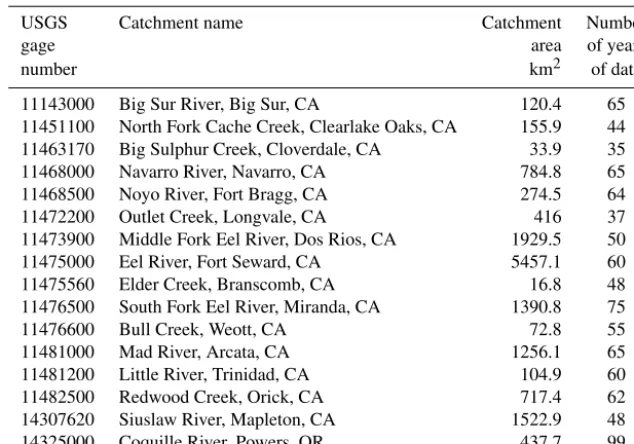
The analyses in this study are performed using United States Geologic Survey daily streamflow data for the set of 16 US catchments from northern California and south-ern Oregon summarized in Table 1. While more frequently sampled discharge data can be used for recession analysis, we use daily data because it is the most common choice in event-scale recession literature. The periods of record for each catchment are visualized in Fig. 1.
The study catchments are relatively steep, forested, and situated within the US western coastal mediterranean cli-mate region (Peel and Finlayson, 2007), which is character-ized by a distinct rainy season (with little or no snowfall), followed by a pronounced dry season during which precip-itation makes a minimal contribution to the water balance (Power et al., 2015; Dralle et al., 2015). While average an-nual rainfall for the study catchments ranges from about 1m to 2m, the highly variable rainfall climatology characteristic of mediterranean regions (Fatichi et al., 2012) might be con-sidered ideal for a recession sensitivity analysis, as catch-ments experience a large range of recession behaviors and wetness states. A typical year of runoff data for Elder Creek near Branscomb, California (USGS Gage: 11475560), is pre-sented in Fig. 2.
2.2 Overview of the methods varied across recession analyses
[image:3.612.50.283.68.237.2]Table 1.Study catchments.
USGS Catchment name Catchment Number
gage area of years
number km2 of data
11143000 Big Sur River, Big Sur, CA 120.4 65
11451100 North Fork Cache Creek, Clearlake Oaks, CA 155.9 44
11463170 Big Sulphur Creek, Cloverdale, CA 33.9 35
11468000 Navarro River, Navarro, CA 784.8 65
11468500 Noyo River, Fort Bragg, CA 274.5 64
11472200 Outlet Creek, Longvale, CA 416 37
11473900 Middle Fork Eel River, Dos Rios, CA 1929.5 50
11475000 Eel River, Fort Seward, CA 5457.1 60
11475560 Elder Creek, Branscomb, CA 16.8 48
11476500 South Fork Eel River, Miranda, CA 1390.8 75
11476600 Bull Creek, Weott, CA 72.8 55
11481000 Mad River, Arcata, CA 1256.1 65
11481200 Little River, Trinidad, CA 104.9 60
11482500 Redwood Creek, Orick, CA 717.4 62
14307620 Siuslaw River, Mapleton, CA 1522.9 48
14325000 Coquille River, Powers, OR 437.7 99
of criteria to confirm the continuation of a hydrograph seg-ment that merits analysis (e.g., a slope or concavity require-ment), (iv) the selection of a fitting methodology by which to analyze a chosen recession. While other choices undoubt-edly have impacts on the characteristics of a population of analyzed recessions, the selection of these four criteria rep-resents the most constrained and fundamental set of method-ological choices to explore.
2.2.1 Nomenclature and symbols used
To concisely describe the combinations of methods tested here, we first represent the four methodological choices with four binary (taking values of 0 or 1) variables:
1. minimum recession length (M) 2. peak selectivity (S)
3. recession concavity (C) 4. fitting method (L).
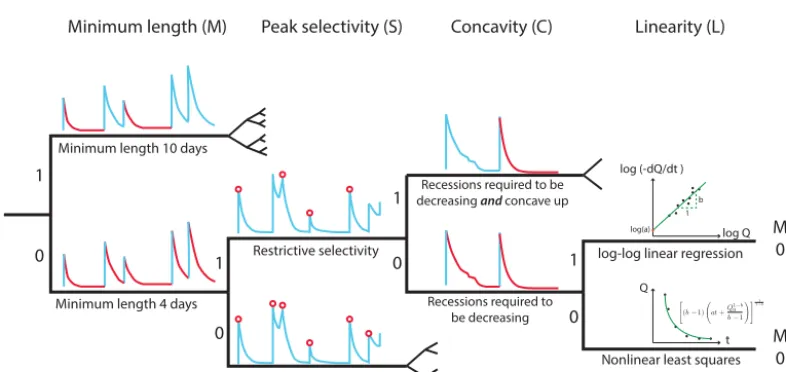
The extraction related variables (M,S, andC) are defined so that a value of 1 corresponds to amore restrictive extraction method; that is, the method choice filters out more recessions if its corresponding variable is 1 than if the variable is 0. For example,M=1 corresponds to a minimum recession length of 10 days, which is more restrictive than a minimum re-cession length of 4 days (M=0). Figure 3 enumerates the 16 method combinations using a decision tree, where each level of the tree sketches the effect of that level’s method choice on the features of extracted recessions.
2.2.2 Defining the minimum allowable length of recession event (M)
Owing to the derivative-based methods developed by Brut-saert and Nieber (1977), most lumped recession analyses do not set a minimum duration recession events. However, nearly all event-scale recession studies set a minimum du-ration for chosen recession periods. Reasons for this choice vary; authors cite the removal of noise from short events (Ye et al., 2014), the necessity of capturing late time flow pro-cesses (Chen and Krajewski, 2015), and data quality con-cerns related to sample size (Shaw, 2016). Event-scale reces-sion analyses have typically chosen a minimum of 4 to 5 days of recession for daily data (e.g., Shaw and Riha, 2012; Biswal and Marani, 2010), although values upwards of 10 days (e.g., Howe, 1966) and as low as 12 h (e.g., McMillan et al., 2014, for high-frequency data) have been used.
Minimum length (M) Peak selectivity (S) Concavity (C) Linearity (L)
log Q log (-dQ/dt )
b 1 log(a)
t Q
(b−1) at+Q1−b
0
b−1
1 1−b
1
1
1
1 0
0
0
0
Permissive selectivity Restrictive selectivity Minimum length 10 days
Minimum length 4 days
Recessions required to be decreasing and concave up
Recessions required to be decreasing
log-log linear regression
N onlinear least squares
Method choices decision tree
MSCL 0101
[image:5.612.100.493.88.274.2]MSCL 0100
Figure 3.Graphical illustration of the 16 method choices. Minimum recession length (M) determines whether extracted recessions are
required to have a minimum length of either 4 (M=0) or 10 days (M=1). Recession peak selectivity (S) determines whether the peak
selection algorithm is highly restrictive (S=1) or relatively permissive (S=0). Recession concavity (C) determines whether recessions are
required to be both decreasingandconcave up (C=1), or simply decreasing (C=0). Finally, Linearity (L) determines whether or not the
values of the recession parametersaandbare determined using linear regression on the plot of log[−dQ/dt] vs. logQ(L=1), or using a
nonlinear least squares fit to the raw recession time series (L=0).
2.2.3 Identifying potential recession starts (S)
Ideally, rainfall data would be used to identify periods of re-cession. However, high-quality precipitation records are of-ten unavailable, and so the majority of event-scale reces-sion analyses rely on flow data alone for recesreces-sion identifica-tion. We therefore only consider methods of recession anal-ysis that can be applied to any daily streamflow record, with or without rainfall data. More stringent extraction methods that require rainfall data would be expected to reduce un-certainty in recession analysis, as extracted recession periods
withrainfall data can reasonably be expected to be a subset of those extractedwithoutrainfall data.
Without rainfall data, recession starts are typically iden-tified by locating days with discharge peaks – that is, times when dQ/dt changes sign from positive to negative. How-ever, some recession starts, while consistent with this defini-tion, do not satisfy other important criteria for robust analysis and should be excluded. Rationales for exclusion might in-clude discarding minor peaks that are small relative to mea-surement error, or which have dynamics that would be ex-pected to be unresolvable on daily timescales, although few authors give a strong justification for their choices in this regard. For example, Ye et al. (2014) discard peak flows less than the 10th flow percentile to filter noise from small events. Mutzner et al. (2013) and Biswal and Marani (2010) choose only recession events where initial flow conditions are greater than mean annual flow in order to avoid “mi-nor events, which may not have significantly increased the
average soil saturation, thus not triggering a significant re-sponse of the groundwater”. Without identifying some jus-tifiable tolerance for noise associated with small peaks, or defining what constitutes a significant groundwater response, it is difficult to objectively determine a peak threshold below which recessions should be excluded from analysis.
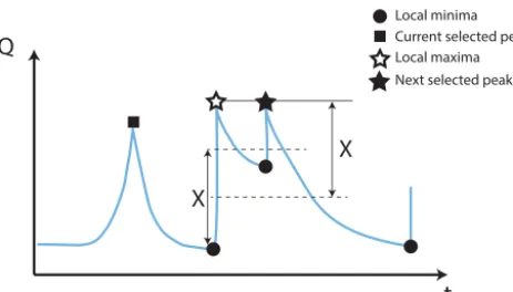
To test the effect of peak filtering decisions on recession analysis, we implement a peak selection procedure that is sensitive to the “distinctness” of any given peak relative to the data around it (Yoder, 2009). Our scheme selects a peak if all of the following are true: (i) it is a local maximum; (ii) it is greater by some threshold amount (X) than the lo-cal minimum lying between it and the previously chosen peak; and (iii) discharge decays to a local minimum by the same threshold amount before the next greater local maxi-mum is found. The peak extraction algorithm is illustrated in Fig. 4. We define the threshold asX=range(Q)/d, where range(Q)=max(Q)−min(Q) is taken over the period of record. Here,dis a tunable parameter that we set to be 50 for highly selective extraction (S=1; only larger, more distinct peaks are analyzed) and set to 500 for less selective extrac-tion (S=0, a broad range of peaks are analyzed).
anal-Q
t
X
X
Current selected peak Local minima
[image:6.612.52.284.65.197.2]Local maxima Next selected peak
Figure 4.Illustration of the peak extraction algorithm. The square represents the most recent recession peak identified for selection. The empty star identifies a local maximum that will not be selected due to the fact that the subsequent recession does not decay by an
amountXbefore the next local maximum. The filled star is selected
as a recession peak because it is at least X greater than the
lo-cal minimum between it and the previously selected recession peak
(square), and is followed by a flow decrease of at leastX.
yses lag recession starts by at least 1 day (Patnaik et al., 2015; Bart and Hope, 2014; Biswal and Marani, 2014), al-though it is not clear that such lagging is necessary to en-able proper interpretation of event-scale dynamics (e.g., Har-man et al., 2009). Fast-flow processes, as well as slow-flow processes, may also contribute to the hypothesized dynamics which generate power law recession behavior. For example, Harman et al. (2009) postulate that heterogeneous transport timescales alone give rise to power law recession dynamics, with no restriction on the “fastest allowable” timescale. With-out a priori information that surface flow processes are a sig-nificant source of runoff generation in a watershed, lagging each recession start may be unnecessary. For example, no surface flow processes have been observed at the Elder Creek watershed in our collection of study watersheds; all runoff is generated by a highly responsive perched water table system (Salve et al., 2012). While adopting either approach – lag-ging the recession time or not – involves some risk, we seek and analyze distinct streamflow peaks without removing any days following the recession start.
2.2.4 Identifying the end of a recession event (C) A number of criteria have been used to determine the end of a recession event. Without a reliable rainfall record, many event-scale analyses halt recession extraction upon the first day where flow does not decrease, that is, as soon as dQ/dt≥0 (e.g., Mutzner et al., 2013). Vogel and Kroll (1996) define the recession end as the first day of increase in the 3-day moving average of streamflow. Shaw and Riha (2012) end the extracted recession 2 days before dQ/dt changes from negative to positive following a recession start. Some studies use the inflection point of the recession curve – the first day following a rainfall event for which the
hydro-graph is concave down – to identify thestartof the extracted recession (Singh and Stall, 1971; Wittenberg and Sivapalan, 1999). A similar concavity criterion, paired with the require-ment of decreasing flow, could also be used to define theend
of a recession event. Exploring every possible combination of the above (and other) methods would lead to an intractably large number of methodological combinations. We therefore define two consensus strategies derived from the above crite-ria.
The first (C=0) considers a recession as any hydrograph segment with dQ/dt <0 following an identified peak. The second, more restrictive strategy (C=1) requires that the raw flow time series is strictly decreasing (again, dQ/dt <0)
andclassified as concave up. A recession day is classified as concave up ifeitherthe raw time seriesora 3-day averaged time series is concave up – that is, if the second difference of either the raw flow time series or a smoothed flow time series is greater than or equal to zero. The inclusion of the criterion based on the 3-day moving average has the effect of including days with small “bumps” in concavity in the raw time series, while consideration of the raw time series ensures inclusion of days immediately after sharply peaked events, which are often classified as convex by the smoothed time series. This simple criterion could serve as an improve-ment to methods that only require dQ/dt <0, which could inadvertently extract highly convex recessions that are likely associated with continued rainfall.
2.2.5 Choosing a fitting procedure (L)
Fitting methods can be broken down into one of three cate-gories: (i) linear regression or enveloping of a binned collec-tion of[log(Q), log(−dQ/dt )]points (e.g., Kirchner, 2009; Parlange et al., 2001); (ii) linear regression or enveloping of a raw collection of[log(Q), log(−dQ/dt )] points (e.g., Brutsaert and Nieber, 1977; Biswal and Marani, 2010); or (iii) nonlinear regression (e.g., Wittenberg, 1994). Within these three general categories, a wide variety of specific re-gression techniques can be applied (e.g., Thomas et al., 2015; Zecharias and Brutsaert, 1988). Importantly, many of these approaches require a large number of data points and are thus unsuitable for event-scale methods.
For event-scale recession fitting, the most popular method is to find a regression line through raw [log(Q), log(−dQ/dt )] point data corresponding to each recession event. There is evidence, however, that nonlinear fitting methods produce more consistent values for recession pa-rameter fits (Wittenberg, 1999; Chen and Krajewski, 2016). Moreover, nonlinear techniques have been used to success-fully parameterize hydrologic models (Müller et al., 2014; Dralle et al., 2016), and to avoid numerical issues associ-ated with computing the time derivative of a flow time series (Rupp and Selker, 2006b).
methodolog-ical dichotomy between linear and nonlinear fitting. Lin-ear fitting (L=1) is performed on the log-transformed val-ues, [log(Q), log(−dQ/dt )]. Values of the flow deriva-tive are computed for each 2-day window (days i and i−1, with 1t=1 day) over the duration of the reces-sion as dQ/dt=(Qi−Qi−1)/1t, with corresponding val-ues ofQcomputed as the average flow value over both days, Q=(Qi+Qi−1)/2 (Brutsaert and Nieber, 1977). Nonlin-ear fitting (L=0) is performed using nonlinear least squares minimization on extracted, non-transformed recession seg-ments.
2.3 Method combination comparisons
In general, only fitted exponents can be reliably compared between different recession events (e.g., Berghuijs et al., 2016; Sawaske and Freyberg, 2014). This is a consequence of a mathematical artifact that impacts fitted values of the re-cession scale parameter, arising when fitting power laws to datasets with arbitrarily chosen scaling (Dralle et al., 2015). The issue can be avoided by setting the recession exponent to a fixed value (e.g., the median; Biswal and Marani, 2010), but this comes at the expense of biasing the fitted values ofadue to constraints on the exponent. Dralle et al. (2015) present a technique that removes the scaling artifact from the recession scale parameter without constraint on the recession exponent. The scale correction procedure begins by first fitting each recession curve to obtain an initial population (of sizen) of recession parametersai andbi. The flow time series is then re-scaled by a constant,Q0, computed as
Q0=exp
n P
i=1
bi−b logai−loga
n P
i=1 bi−b
2
, (2)
where loga is the mean of the natural logarithm of theai, andb is the mean of the bi. Following re-scaling, the flow time series is re-fit to the power law recession model. While the recession exponent is scale-independent, the recession scale parameter will be altered by the scaling procedure in such a way as to eliminate artifactual linear correlation be-tween logaandb. The resultant population of recession scale parameters has units of inverse time and has been shown em-pirically to correlate strongly with measures of catchment wetness (Dralle et al., 2015).
With this in mind, we choose three primaryrecession mea-suresfor comparison between recession events: the recession exponent (b), the scale-corrected (Dralle et al., 2015) reces-sion scale parameter (a), and the recesreces-sion time (TR), defined by Stoelzle et al. (2013) as the amount of time required for flow levels to decline from the median flow to the 10th flow percentile. The measureTR, which depends on bothaandb, belongs to a class of widely calculated recession timescales for the general, nonlinear form of Eq. (1) (e.g., Stoelzle et al., 2013; Westerberg and McMillan, 2015).
To see how methodological choices might impact the in-terpretation ofa,b, andTR, we organize our analysis around four primary questions, which were outlined in the introduc-tion and are detailed in the following secintroduc-tions.
2.3.1 Research question 1 – how do methodological choices impact the overall quality of individual recession fits?
Fit quality is one measure of confidence in the estimated value for each recession measure. Testing event-scale reces-sion theories that predict specific values for recesreces-sion mea-sures (e.g., Biswal and Marani, 2010) can be expected to be constrained by the degree of this confidence. This question looks to identify method combinations that consistently pro-duce high-quality fits, and thus high confidence in recession parameter estimates.
We report two measures of the overall quality of reces-sion fits as a function of combinations of method choices. First we compute the mean average percent error (abbrevi-ated as MAPE and denoted mathematically as EMAP) for each method combination, across all catchments. MAPE is computed as
EMAP= 1 N
N X
i=1
Qi− ˆQi
Qi
, (3)
whereQi andQˆi are the observed and predicted flows on
theith day following the start of the recession event. (Note that comparing goodness of fit usingR2is not appropriate, because one of our fitting methods is nonlinear (Kvalseth, 1985).) We also report, for each method, the percentage of all fits that yield “non-physical” estimates for the recession parameters, which we define asb <0. In all subsequent anal-yses, the recession parameters are filtered so thatb≥0 (b <0 occurs for less than 3 % of all recession events).
2.3.2 Research question 2 – area,b, andTR
“characteristic” across various methodological choices?
That is, do catchments rank in a similar order according to different statistical measures (in the present study, the median and interquartile range) of the populations ofa,b, andTR across the 16 method combinations (cf. Stoelzle et al., 2013)? The results of comparative hydrologic studies (e.g., Bogaart et al., 2016), which rely on relative relationships between recession measures, can be expected to be affected by any methodological sensitivity demonstrated here.
measure of central tendency and the interquartile range as a measure of variability, both of which are robust against the biasing effects of occasional outlier fits. Following Stoel-zle et al. (2013), we compute Spearman rank correlation co-efficients by ranking catchments between all method com-bination pairs based on the following measures (recession characteristics): median(a), median(b), median(TR), IQR(a), IQR(b), and IQR(TR), where IQR is the interquartile range. The rank correlation can take a value between −1 and 1, where a rank correlation of 1 indicates that two method com-binations produce identical rankings and a rank correlation of −1 indicates that two method combinations produce ex-actly opposite rankings.
Even if the absolute magnitudes of the values of a, b, andTR vary between the method combinations, these rank tests will determine whether catchments rank in the same or-der by the recession characteristic for all methods. Determin-ing the consistency of such ranked comparisons has implica-tions for efforts to develop effective metrics for catchment classification, where relative differences in recession charac-teristics have been used to compare or categorize catchments (e.g Bogaart et al., 2016; Mutzner et al., 2013; Guzmán et al., 2015).
2.3.3 Research question 3 – for each catchment, are the empirical frequency distributions ofa,b, andTR
statistically similar across method combinations, and, if not, what method choices have the greatest impact on recession parameter distributions?
Event-scale theories of the streamflow recession suggest that, beyond measures of central tendency, higher-order moments of recession parameter distributions (such as the variance) should vary in systematic ways, depending on climate or catchment physiographic properties (Biswal and Nagesh, 2014; Harman et al., 2009). By addressing research ques-tion 3, we seek to identify the methodological choices which could most significantly impact testing of event-scale reces-sion theories.
While shifts in the Spearman rank correlation between method combinations allow a comparative analysis of the effects of method choice, they do not provide information about variations in the specific values of the recession pa-rameters obtained by each method. To address the specific values of the recession parameters, which is important for testing theories that make such specific predictions (Biswal and Marani, 2010; Brutsaert, 1994), we therefore also ex-plore the empirical frequency distributions of parameter pop-ulations estimated with each methodological combination.
We first illustrate general patterns ofa,b, andTR, across all method combinations with Tukey box plots for a single representative catchment – the Elder Creek watershed, a trib-utary of the Eel River in northern California. These plots pro-vide visual representation of theobserveddifference between the character of recession measure distributions for different
0 1
Nov Dec Jan/01
4-day minimum, less restrictive extraction
Shared
Not shared
(a)
(d)
(c)
(b)
0 1
0 1
0 1
10-day minimum, more restrictive extraction
Dischar
ge [m
3s
]
[image:8.612.311.546.67.311.2]-3
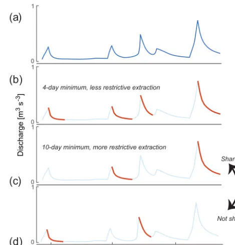
Figure 5.Example recession extraction from the hydrograph(a)
using a less restrictive methodM=0(b) and a more restrictive
methodM=1(c). The recessions identified by the more restrictive
method will be “shared” by the two methods, in the sense that they will by definition also be identified by the less restrictive method.
Recessions identified by only the less restrictive method (d) are
classified as “unshared”.
method combinations. However, they do not represent the ab-solute effect of changing individual method choices. This is because more restrictive extraction procedures produce pop-ulations of recessions that are a subset of the poppop-ulations gen-erated by less restrictive extraction measures. For example, fixing all other method choices, recessions extracted with a minimum length of 10 days must be a subset of recessions extracted with a minimum length of 4 days. This “dilutes” the true effect of the shift in choice of minimum recession length on the recession measures derived from the two re-sulting populations.
One way to isolate the absolute effect of a given method choice is to compare recessions that aresharedbetween the restrictive choice and non-restrictive choice, to those that are
ex-traction). Differences between these disjoint “shared” and “unshared” sets of recessions embody the absolute effect of an individual method choice on a recession measure. Reces-sion measures between the two groups should be compara-ble if the particular recession measure is not sensitive to the method choice.
We compare shared and unshared recession measure dis-tributions in two ways. First, for a high-level overview, we show Tukey box plots of shared vs. unshared distributions of the recession exponent (b) for a single catchment (the El-der Creek watershed) for two recession extraction choices (minimum length and concavity). We then use a two-sided Mann–WhitneyU test (Mann and Whitney, 1947) to com-pare shared vs. unshared distributions for each recession measure across all method choices and all catchments. The null hypothesis for this non-parametric test is that the shared and unshared distributions are sampled from the same pop-ulation. For a given catchment and for each method choice, we computepvalues for the Mann–WhitneyUtest by com-paring shared to unshared distributions for each of the eight combinations of the other method choices. If the test rejects the null hypothesis, then we conclude that the method choice significantly changes the distribution of the recession mea-sure (note: we also compare populations between linear and nonlinear fitting; although it is not a “shared” vs. “unshared” comparison, the two fitting methods nonetheless produce dis-tinct distributions for the recession measures).
For each catchment, we then rank the four method choices by the number of Mann–Whitney U tests (eight tests for each method choice) that detect significant differences be-tween shared and unshared distributions. A method choice is assigned a higher rank if more shared/unshared compar-isons detect significant differences. We use this rank as an indicator of the sensitivity of a recession measure to a given method choice. We perform this procedure for all recession measures,a,b, andTR. Since each measure requires 512 total comparisons (16 catchments×8 tests×4 method choices), we apply a Bonferroni correction for the criticalp value of each test, which is required when a statistical test is applied many times for multiple comparisons (Abdi, 2007). For an overall level of significance of α=0.05, the correction re-quires a criticalpvalue for each test set top=α/512. 2.3.4 Research question 4 – can methodological choices
affect features of the observed relationship between measures of catchment wetness and the recession scale parameter?
Overall, few studies have attempted to tease apart the con-vergent predictions of power law recession theories. Some works informed by Biswal and Marani (2010) demonstrate a relationship between measures of antecedent catchment wetness and the power law scale parameter (e.g., Bart and Hope, 2014; Biswal and Nagesh, 2014; Patnaik et al., 2015), although explicit connections to wetted channel network
expansion and contraction still require elucidation (Ghosh et al., 2016). Whatever its physical basis, we observe similar correlations between measures of antecedent wetness and the scale-corrected recession scale parameter. To demonstrate that method choices can significantly impact the quantita-tive nature of such emergent relationships, we explore the functional relationship between the recession scale parame-ter and a measure of antecedent wetness for the Elder Creek catchment for three methodological combinations. The an-tecedent wetness measure (W) is computed as a weighted sum of streamflow prior to each recession event:
W=
60
X
i=1
0.95iQi, (4)
wherei is the number of days prior to the start of the re-cession event. The weighting coefficient, 0.95i, is included to discount the effect of less recent events on the catchment wetness state. Following recession extraction and fitting, a re-gression line is fit to observed log–log linear relationships be-tweenaandWand the resulting regression slopes are com-pared between the three method combinations.
3 Results
While the lengths of record for study catchments vary from 35 to 99 years, we find that subsetting flow records and re-performing analyses does not significantly impact our find-ings. We also find that, at confidence levelp=0.05, approx-imately 6 % of the (16 catchments×16 method combina-tions×3 recession measures)=768 populations of recession measures exhibit significant trends over time. At a confidence level of 0.05, one would expect 5 % of the tests to flag sig-nificance purely by chance. We conclude that any potential trends in recession parameters over time will have a minimal impact on the results of this study.
3.1 Recession fit quality
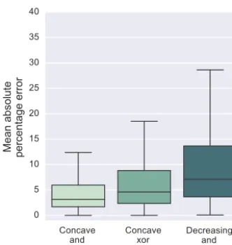
The box plots in Fig. 6 are generated using computed MAPE values for all fits across all catchments. The boxes are grouped using certain combinations of linearity and concav-ity, the two method choices found to be the strongest con-trollers of fit quality. There is a clear increase in fit quality as-sociated with extraction of concave-only recessions and use of nonlinear fitting procedures.
Concave and nonlinear
Concave xor nonlinear
Decreasing and linear 0
5 10 15 20 25 30 35 40
[image:10.612.84.250.65.240.2]Mean absolute percentage error
Figure 6.Mean absolute percentage error (MAPE) lumped across catchments by three groups: concave only recessions with nonlinear fitting; concave recessions or nonlinear fitting but not both (denoted using the logical “exclusive or” operator, “xor”); and decreasing re-cessions (without the concavity requirement) and linear fitting pro-cedures.
but found few patterns related to individual method choices. Therefore, we present aggregated box plots of the Spear-man rank correlation for each of the recession characteris-tics. Overall, none of the rank correlations were negative. The most “characteristic” measure, in the sense that its ability to rank catchments is least sensitive to the method choice, is median(a).
3.3 Recession measure distributions
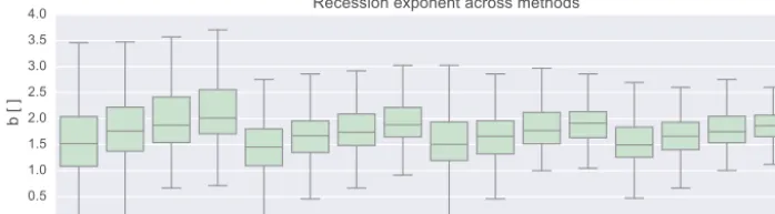
Figure 8 presents box plots of the three recession measures across all method combinations for the Elder Creek study catchment. For any given method combination, variability in the recession measures can be significant. The recession ex-ponentbregularly falls betweenb=1 andb=2.5, while in-terquartile ranges foraandTRtypically span upwards of an order of magnitude.
Figure 9 is provided to help illustrate the comparisons be-tween shared and unshared distributions of recession mea-sures. In this case, we compare recession exponent shared vs. unshared distributions for the Elder Creek watershed for the minimum recession length method choice and the con-cavity method choice. The light green boxes represent the distribution of the recession exponent for shared recessions, while the dark green boxes represent the unshared population of recession exponent values (extracted by only the less re-strictive procedure). The horizontal axes in each subplot enu-merate the eight possible combinations of the other method choices, showing how these shared and unshared distribu-tions vary for different combinadistribu-tions of the other method variables. Significant differences between the shared and un-shared distributions as determined by a two-sided Mann–
med(a) med(b) med(TR) IQR(a) IQR(b)
Recession characteristic
0.0 0.2 0.4 0.6 0.8 1.0
R
an
k
co
rr
el
at
io
n
Box plots of Spearman rank correlation
IQR(TR)
Figure 7.Box and whisker plots of Spearman rank correlations for
all six descriptive measures of the distributions ofa,b, andTR. Per
characteristic, there are 15×16=240 unique pairwise comparisons
between method combinations.
WhitneyUtest are indicated with red highlighting in Fig. 9. Two of the eight unshared/shared distribution pairs are identi-fied as significantly different for the minimum length method choice, while eight of the eight pairs are identified as differ-ent for the concavity choice.
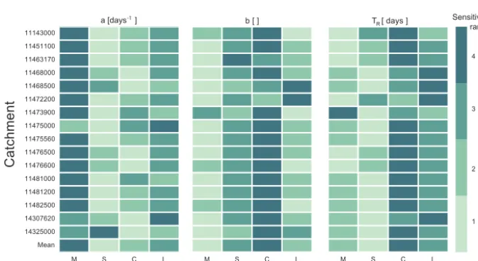
The results from Fig. 9 feed into the larger shared vs. un-shared analysis for all recession measures across all water-sheds presented in Fig. 10. This figure plots outcomes of all Mann–WhitneyU tests between shared and unshared distri-butions for each recession measure, for all method choices, and for all catchments. The Elder Creek (catchment number 11475560) recession exponent distributions in Fig. 9 corre-spond to the recession exponent subplot (center) of Fig. 10, row 11475560, columnsMandC. In agreement with Fig. 9, the recession exponent is most significantly affected by the choice to extract only concave recessions, and less so by the minimum recession length. The strong dependence on con-cavity demonstrated in Fig. 9 manifests in Fig. 10 as the very dark rectangle in the concavity column of the recession ex-ponent parameter for the Elder Creek catchment, gage num-ber 11475560.
3.4 Catchment wetness and the recession scale parameter
[image:10.612.312.544.66.218.2]0000 0001 0010 0011 0100 0101 0110 0111 1000 1001 1010 1011 1100 1101 1110 1111
0.0 0.5 1.0 1.5 2.0 2.5 3.0 3.5 4.0
b [ ]
Recession exponent across methods
MSCL MSCL...
0000 0001 0010 0011 0100 0101 0110 0111 1000 1001 1010 1011 1100 1101 1110 1111
10-6
10-5
10-4
10-3
10-2
10-1
100
101
a [ days
-1 ]
Recession scale parameter across methods
MSCL MSCL...
0000 0001 0010 0011 0100 0101 0110 0111 1000 1001 1010 1011 1100 1101 1110 1111 Method
10-2
10-1 100
101
102
103
104
TR
[ days ]
Recession time across methods
MSCL MSCL...
[image:11.612.125.474.100.196.2]Recession measure distributions for Elder Creek watershed
Figure 8.Box plots fora,b, andTRacross all method combinations for Elder Creek watershed.
4 Discussion
4.1 Recession fit quality
The pattern in Fig. 6 hints at a hierarchy of the importance of method choices in terms of their impact on the “quality” of extracted recessions and their corresponding power law fits. Specifically, we found that the concavity (C) and lin-earity (L) method choices roughly subdivide the results into three groups. The worst fits observed were those performed without the concavity requirement (only the decreasing re-quirement) and with linear regression. Fits that use concave recessions or nonlinear fitting, but not both, are of intermedi-ate quality. The best fits are those that combined the concav-ity requirement with nonlinear regression. Overall, the results
suggest an additive increase in goodness of fit associated with the concavity requirement and nonlinear fitting.
0 1 2 3 4 5
Recession exponent (b)
Minimum recession length (M) Concavity (C)
Eight combinations of other method choices Eight combinations of other method choices
Shared Unshared
Red highlight means the Mann–Whitney U test detected a significant difference between shared and unshared distributions.
[image:12.612.125.473.84.195.2]Example shared vs. unshared distributions for Elder Creek watershed
Figure 9.Box plots comparing recession exponent shared vs. unshared distributions for minimum recession length and concavity method
choices for Elder Creek. Each subplot corresponds to a particular method choice; the shared boxes are generated with thebvalues from the
recessions shared between the more and less restrictive values of the method choice for that subplot. The unshared boxes are those values
ofbfrom the recessions extracted byonlythe less restrictive value of the subplot method choice. The independent axis enumerates the eight
combinations of the method choices other than the subplot method choice.
M S C L
Mean 14325000 14307620 11482500 11481200 11481000 11476600 11476500 11475560 11475000 11473900 11472200 11468500 11468000 11463170 11451100 11143000
a [days-1]
M S C L
b [ ]
M S C L
T [ days ]
1 2 3 4
R
In
cr
easing
sen
si
tiv
ity
Catchment
Method Method Method
Sensitivity rank
Figure 10.Results of Mann–WhitneyUtest sensitivity analysis. Each row represents 1 of the 16 study catchments, each subplot one of
the three recession measuresa,b, orTR, and each subplot column one of the four methodological choices (MSCL). Each cell is colored
by a sensitivity rank. A cell shading of 4 (darkest) means that method choice had the highest number of significantly different shared and unshared distributions for that recession measure in that catchment, indicating that the particular recession measure is highly sensitive to the corresponding method choice.
fact, the often-used definition of flow recession – that the flow derivative is negative – could be misleading; the sim-ple dynamical system model developed by Kirchner (2009) predicts that streamflow can decrease during precipitation events. The use of improved, flow-derived recession extrac-tion methods, such as the concavity requirement, could re-duce the frequency of “false” recession extraction, increasing the quality of recession measure estimates.
Beyond the tendency to produce lower-quality fits, the lin-ear fitting procedures applied in the majority of recession studies have other well-documented drawbacks. Linear re-gression on log-transformed flow values disproportionately weights errors for smaller model values, creating a risk of
[image:12.612.130.467.294.478.2]3 4 5 6 7 8 9 10 11
log(W)
−12 −10 −8 −6 −4 −2 0 2 4 6
lo
g(
a
)
Decreasing recessions, linear fitting , 4-day min leng th, less selective peak selection
3 4 5 6 7 8 9 10 11
log(W)
Concave recessions, nonlinear fitting , 4-day min leng th, less selective peak selection
3 4 5 6 7 8 9 10 11
log(W)
Concave recessions, nonlinear fitting , 10-day min leng th, more selective peak selection
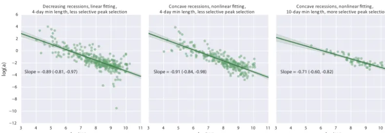
[image:13.612.102.497.65.201.2]Slope = -0.89 (-0.81, -0.97) Slope = -0.91 (-0.84, -0.98) Slope = -0.71 (-0.60, -0.82)
Figure 11.The recession scale parameter plotted against antecedent catchment wetness for three method combinations, together with a linear fit for each point cloud, and a 95 % confidence interval for each fitted slope.
tightly constrained values, but for other more variable reces-sion measures, such asa, this choice could also be opaque, and differing initial conditions could lead to differing reces-sion parameter estimations.
4.2 Recession measures are characteristic
We find that the medians and IQRs of a,b, andTRare all fairly characteristic, though to varying degrees. All rank cor-relations are positive, indicating that, at worst, no method combination predicts a characteristic ranking that is inverted relative to another method combination. Median(a) is more characteristic than median(b) or median(TR), and each IQR is less characteristic than its corresponding median. One might expect that median(a) is highly characteristic because it spans many orders of magnitude, while other parameters are more tightly constrained. However, the derived measure TRalso has a wide range but does not display the same level of rank stability asa.
The relatively stable ranking of catchments by recession measures has potential implications for testing event-scale recession theory. Recent work by Harman et al. (2009) hy-pothesizes thatbcan be interpreted as a measure of the di-versity of water transport timescales throughout the various parts of the catchment. In this framework, measures of vari-ability ofbcould be interpreted as representative of the “real-izable” range of catchment states, with respect to the relative dominance of various water transit times in the catchment. Strongly characteristic measures of b suggest the potential to use the recession exponent to develop relative measures of catchment complexity, if the Harman et al. (2009) theory applies to catchment populations.
Results also provide support for application of the reces-sion scale parameter scale-correction procedure presented by Dralle et al. (2015). Medians of the scale-corrected recession scale parameters rank catchments more consistently than all other recession characteristics. Moreover, the fact thatahas units of inverse time suggests it can be interpreted physically in a manner similar to more commonly computed response
timescales, such asTR(e.g., Stoelzle et al., 2013; Westerberg and McMillan, 2015). In fact, the median and IQR ofTRare the least consistent catchment ranking characteristics. Con-sidering thatTR is a measure derived from both a and b, it has likely inherited catchment ranking uncertainty from both these parameters. Numerous derived recession measures have been used for comparative catchment analysis (Sawaske and Freyberg, 2014; Berghuijs et al., 2016; Stoelzle et al., 2013), and the findings here suggest a trade-off; the develop-ment of more complex derived measures comes at the risk of compounding uncertainty.
4.3 Comparing distributions of recession measures
Patterns in the recession measures for Elder Creek plotted in Fig. 8 are generally representative of the patterns observed in the other 15 study catchments. The four-step repeating pat-tern forb seen in Fig. 8 indicates that concavity and linear-ity play important roles in shifting the distributions of the recession exponent. When other methodological choices are fixed, nonlinear fitting and concavity both produce notice-ably higher values for the recession exponent. Without the concave requirement, the “decreasing only” extraction pro-cedures will produce lower values due to decreased concav-ity. Table 2 supports this conclusion; the concavity require-ment greatly decreases the number of “non-physical” (b <0) extracted recessions.
reces-Table 2.Fraction of recessions with non-physical recession
expo-nent (b <0) for each method combination.
Method combination Fraction of fits
(MSCL) withb <0
0 (0000) 0.114
1 (0001) 0.035
2 (0010) 0.070
3 (0011) 0.005
4 (0100) 0.097
5 (0101) 0.024
6 (0110) 0.059
7 (0111) 0.003
8 (1000) 0.032
9 (1001) 0.002
10 (1010) 0.013
11 (1011) 0.0
12 (1100) 0.016
13 (1101) 0.001
14 (1110) 0.004
15 (1111) 0.0
sion timescales (commonly referred to as the “recession con-stant”) extracted from linear reservoir models (e.g., Sánchez-Murillo et al., 2015; Botter et al., 2013). The observed me-dian values of bandTRare also consistent with those typ-ically found in lumped recession analyses (e.g., Tague and Grant, 2004; Palmroth et al., 2010; Szilagyi et al., 2007; Wang, 2011; Stoelzle et al., 2013; McMillan et al., 2014).
A pattern of shorter whiskers from left to right in Fig. 8 shows that the variability of the recession measures decreases as extraction procedures become more restrictive. For a min-imum recession length of 10 days and highly selective peak filtering (M=1,S=1), this decrease in variability is likely due to the fact that the collection of extracted recessions be-comes less “diverse” as the extraction method bebe-comes more restrictive, as suggested by Stoelzle et al. (2013). As com-pared to minimum length and peak selectivity, which had a minimal impact on fit quality (see Fig. 6), the larger vari-ability for non-concave data paired with nonlinear fitting is due, at least in part, to more noise from persistent rainfall during the recession. This suggests that peak size and reces-sion length data quality concerns cited by some authors (e.g., Ye et al., 2014; Shaw, 2016) could be augmented to consider fitting methods and the “quality” of the shape of extracted recessions.
Patterns displayed in Fig. 9 are largely similar to distri-butions of b in other watersheds. Whiskers are shorter for “shared” distributions for minimum length (as well as for se-lectivity, although it is not plotted here to simplify the pre-sentation). This could be because very large storms and very long recessions, which are more likely to be shared, repre-sent the asymptotic behavior of the catchment response as-sociated with more extreme states. Despite this disparity in
variability between shared and unshared distributions, the Mann–WhitneyU test identified only two of the eight dis-tribution pairs as significantly distinct from one another, sug-gesting moderate sensitivity ofbto the minimum recession length choice. The second subplot displays shared and un-shared distributions for the concavity method choice, which again emerges as the most important choice for determining the absolute magnitude ofb. The Mann–WhitneyUtest iden-tified all eight distribution pairs as significantly distinct, in-dicating high sensitivity ofbto the concavity method choice. Whereas Fig. 6 indicated certain method choices play an important role in determining quality of fit, Fig. 10 demon-strates that other choices could play a more important role in determining realized values ofa andb. This finding makes it difficult to determine the “best” method combination. Whereas concavity and linearity were the dominant drivers of goodness of fit, it is selectivity and concavity that exert the strongest control over the distribution ofb. Minimum re-cession length seems to exert the strongest control over the distribution of the recession scale parameter (a). Along with the inconsistencies in controls on each recession measure, we also note that some recession measures are uniformly sensitive to a given method for all catchments (e.g., concav-ity strongly affectsbfor almost all catchments), while oth-ers seem to vary between catchments. For example, linear-ity exerts a strong control on the distribution ofbfor catch-ment 11468500 (Noyo River), but apparently makes very lit-tle difference for catchment 11143000 (Big Sur River). 4.4 The relationship between catchment antecedent
wetness and the recession scale parameter
Despite moderate sensitivity to concavity and linearity in the Elder Creek data (catchment 11475560) displayed in Fig. 10, the first two fits in Fig. 11 are not statistically different as shown by 95 % confidence intervals for the fitted slopes. The slope on the third plot differs significantly from the first two, likely due to the fact that the population of recessions orig-inates from a highly selective extraction procedure that trig-gersa’s strong sensitivity to the minimum recession length method choice. This highlights the potential for recession ex-traction bias in parameter populations; without good cause to discard smaller or shorter recessions, such choices can lead to quantitatively different interpretations of recession param-eter values. In general, Fig. 11 demonstrates that quantitative validation of recession theories that predict emergent rela-tionships between recession measures and catchment state may be hindered by uncertainty relating to methodological choices.
4.5 Methodological recommendation
[image:14.612.92.242.95.305.2]re-cession measureais highly sensitive to the minimum length choice, and the recession exponent is highly sensitive to con-cavity and moderately sensitive to peak selectivity, as demon-strated by Figs. 8 and 10. Taken all together, we conclude that this suggests an ideal combination of method choices that will both maximize fit quality and minimize bias in the “type” of recession identified for fitting: 4-day mini-mum length (M=0), permissive recession peak selectivity (S=0), concavity requirement (C=1), and nonlinear least squares fitting (L=0).
5 Conclusion
This study quantified the sensitivity of the power law stream-flow recession parametersa andbto four common method-ological choices made during recession extraction and fitting. While rankings of study catchments in terms of the descrip-tive statistics of a and b were relatively insensitive to the methods used, individual method choices did significantly impact observed parameter distributions, though each param-eter had a distinct sensitivity profile. These results highlight the importance of accounting for methodological uncertainty when performing event-scale recession analysis.
6 Data availability
All streamflow data used for this study can be found on the website for United States Geological Survey (http:// waterdata.usgs.gov/nwis). Code used to perform this analysis is being developed as a web application for the Consortium of Universities Allied for Water Research (CUAHSI) and is preliminarily available at https://github.com/daviddralle/ tethysapp-recession_analyzer.
Author contributions. David N. Dralle conceived of the study, per-formed analysis, and was the primary author. Nathaniel J. Karst con-ceived of the study, performed analysis, and contributed to writing. Kyriakos Charalampous curated recession parameter datasets and performed analysis. Andrew Veenstra performed analysis and de-veloped recession analysis software. Sally E. Thompson contributed to writing and editing.
Acknowledgements. The authors would like to thank Davit Khacha-tryan and Laurel Larsen for helpful conversations concerning some aspects of the statistical and sensitivity analyses presented here.
Edited by: J. Seibert
Reviewed by: M. Stoelzle and one anonymous referee
References
Abdi, H.: The Bonferonni and Šidák corrections for multiple com-parisons, Encyclop. Measure. Stat., 3, 103–107, 2007.
Bart, R. and Hope, A.: Inter-seasonal variability in base-flow recession rates: The role of aquifer antecedent storage in central California watersheds, J. Hydrol., 519, 205–213, doi:10.1016/j.jhydrol.2014.07.020, 2014.
Basso, S., Schirmer, M., and Botter, G.: On the emergence of heavy-tailed streamflow distributions, Adv. Water Resour., 82, 98–105, 2015.
Berghuijs, W., Hartmann, A., and Woods, R.: Streamflow sensitivity to water storage changes across Europe, Geophys. Res. Lett., 43, 1980–1987, doi:10.1002/2016GL067927, 2016.
Biswal, B. and Marani, M.: Geomorphological origin of
recession curves, Geophys. Res. Lett., 37, L24403,
doi:10.1029/2010GL045415, 2010.
Biswal, B. and Marani, M.: ‘Universal’ recession curves and their geomorphological interpretation, Adv. Water Resour., 65, 34–42, doi:10.1016/j.advwatres.2014.01.004, 2014.
Biswal, B. and Nagesh, K. D.: Study of dynamic behaviour
of recession curves, Hydrol. Process., 28, 784–792,
doi:10.1002/hyp.9604, 2014.
Bogaart, P. W., v. d. Velde, Y., Lyon, S. W., and Dekker, S. C.: Streamflow recession patterns can help unravel the role of cli-mate and humans in landscape co-evolution, Hydrol. Earth Syst. Sci., 20, 1413–1432, doi:10.5194/hess-20-1413-2016, 2016. Botter, G., Basso, S., Rodriguez-Iturbe, I., and Rinaldo, A.:
Re-silience of river flow regimes, P. Natl. Acad. Sci. USA, 110, 12925–12930, 2013.
Boussinesq, J.: Essai sur la théorie des eaux courantes, vol. 2, Im-primerie nationale, Paris, France, 1877.
Boussinesq, J.: Recherches théoriques sur l’écoulement des nappes d’eau infiltrées dans le sol et sur le débit des sources, Journal de Mathématiques Pures et Appliquées, 10, 5–78, 1904.
Brutsaert, W.: The unit response of groundwater outflow
from a hillslope, Water Resour. Res., 30, 2759–2763,
doi:10.1029/94WR01396, 1994.
Brutsaert, W. and Nieber, J. L.: Regionalized drought flow hydro-graphs from a mature glaciated plateau, Water Resour. Res., 13, 637–648, doi:10.1029/WR013i003p00637, 1977.
Chen, B. and Krajewski, W.: Analysing individual recession events: sensitivity of parameter determination to the calculation proce-dure, Hydrolog. Sci. J., 61, 2887–2901, 2016.
Chen, B. and Krajewski, W. F.: Recession analysis across scales: The impact of both random and nonrandom spatial variability on aggregated hydrologic response, J. Hydrol., 523, 97–106, 2015. Clark, M. P., Rupp, D. E., Woods, R. A., Tromp-van Meerveld, H. J.,
Peters, N. E., and Freer, J. E.: Consistency between hydrological models and field observations: linking processes at the hillslope scale to hydrological responses at the watershed scale, Hydrol. Process., 23, 311–319, doi:10.1002/hyp.7154, 2009.
Dralle, D., Karst, N., and Thompson, S. E.:a,bcareful: The
chal-lenge of scale invariance for comparative analyses in power law models of the streamflow recession, Geophys. Res. Lett., 42, 9285–9293, doi:10.1002/2015GL066007, 2015.
Fatichi, S., Ivanov, V. Y., and Caporali, E.: Investigating Interan-nual Variability of Precipitation at the Global Scale: Is There a Connection with Seasonality?, J. Climate, 25, 5512–5523, doi:10.1175/JCLI-D-11-00356.1, 2012.
Ghosh, D. K., Wang, D., and Zhu, T.: On the transition of base flow recession from early stage to late stage, Adv. Water Resour., 88, 8–13, 2016.
Guzmán, P., Batelaan, O., Huysmans, M., and Wyseure, G.: Com-parative analysis of baseflow characteristics of two Andean catchments, Ecuador, Hydrol. Process., 29, 3051–3064, 2015. Hall, F. R.: Base-flow recessions – a review, Water Resour. Res., 4,
973–983, doi:10.1029/WR004i005p00973, 1968.
Harman, C. J., Sivapalan, M., and Kumar, P.: Power law catchment-scale recessions arising from heterogeneous lin-ear small-scale dynamics, Water Resour. Res., 45, W09404, doi:10.1029/2008WR007392, 2009.
Howe, J. W.: Recession characteristics of Iowa streams, Studies in Engineering Bulletin, The University of Iowa, Iowa City, 1–6, 1966.
Huyck, A. A. O., Pauwels, V., and Verhoest, N. E. C.: A base flow separation algorithm based on the linearized Boussinesq equa-tion for complex hillslopes, Water Resour. Res., 41, W08415, doi:10.1029/2004WR003789, 2005.
Kirchner, J. W.: Catchments as simple dynamical systems: Catchment characterization, rainfall-runoff modeling, and do-ing hydrology backward, Water Resour. Res., 45, W02409, doi:10.1029/2008WR006912, 2009.
Kvalseth, T. O.: Cautionary Note aboutR2, Am. Statist., 39, 279–
285, doi:10.2307/2683704, 1985.
Lamb, R. and Beven, K.: Using interactive recession curve analysis to specify a general catchment storage model, Hydrol. Earth Syst. Sci., 1, 101–113, doi:10.5194/hess-1-101-1997, 1997.
Mann, H. B. and Whitney, D. R.: On a test of whether one of two random variables is stochastically larger than the other, in: The annals of mathematical statistics, Institute of Mathematical Statistics, Ann Arbor, Michigan, 50–60, 1947.
McMillan, H., Gueguen, M., Grimon, E., Woods, R., Clark, M., and Rupp, D. E.: Spatial variability of hydrological processes and
model structure diagnostics in a 50 km2catchment, Hydrol.
Pro-cess., 28, 4896–4913, doi:10.1002/hyp.9988, 2014.
Miller, D. M.: Reducing transformation bias in curve fitting, Am. Stat., 38, 124–126, doi:10.2307/2683247, 1984.
Motulsky, H. J. and Ransnas, L. A.: Fitting curves to data using nonlinear regression: a practical and nonmathematical review, FASEB J., 1, 365–374, 1987.
Müller, M. F., Dralle, D. N., and Thompson, S. E.: Analytical model for flow duration curves in seasonally dry climates, Water Re-sour. Res., 50, 5510–5531, doi:10.1002/2014WR015301, 2014. Mutzner, R., Bertuzzo, E., Tarolli, P., Weijs, S. V., Nicotina,
L., Ceola, S., Tomasic, N., Rodríguez-Iturbe, I., Parlange, M. B., and Rinaldo, A.: Geomorphic signatures on Brutsaert base flow recession analysis, Water Resour. Res., 49, 5462–5472, doi:10.1002/wrcr.20417, 2013.
Palmroth, S., Katul, G. G., Hui, D., McCarthy, H. R., Jackson, R. B., and Oren, R.: Estimation of long-term basin scale evapotran-spiration from streamflow time series, Water Resour. Res., 46, W10512, doi:10.1029/2009WR008838, 2010.
Parlange, J. Y., Stagnitti, F., Heilig, A., Szilagyi, J., Parlange, M. B., Steenhuis, T. S., Hogarth, W. L., Barry, D. A., and Li, L.: Sudden
drawdown and drainage of a horizontal aquifer, Water Resour. Res., 37, 2097–2101, 2001.
Patnaik, S., Biswal, B., Kumar, D. N., and Sivakumar, B.: Effect of catchment characteristics on the relationship between past dis-charge and the power law recession coefficient, J. Hydrol., 528, 321–328, 2015.
Pattyn, F. and Van Huele, W.: Power law or power flaw?, Earth Surf. Proc. Land., 23, 761–767, doi:10.1002/(SICI)1096-9837(199808)23:8<761::AID-ESP892>3.0.CO;2-K, 1998. Peel, M. C., Finlayson, B. L., and McMahon, T. A.: Updated
world map of the Köppen-Geiger climate classification, Hy-drol. Earth Syst. Sci., 11, 1633–1644, doi:10.5194/hess-11-1633-2007, 2007.
Power, M. E., Bouma-Gregson, K., Higgins, P., and Carlson, S. M.: The Thirsty Eel: Summer and Winter Flow Thresholds that Tilt the Eel River of Northwestern California from Salmon-Supporting to Cyanobacterially Degraded States, Copeia, 2015, 200–211, doi:10.1643/CE-14-086, 2015.
Rupp, D. E. and Selker, J. S.: On the use of the Boussinesq equation for interpreting recession hydrographs from sloping aquifers, Water Resour. Res., 42, W12421, doi:10.1029/2006WR005080, 2006a.
Rupp, D. E. and Selker, J. S.: Information, artifacts, and noise in
dQ/dt−Qrecession analysis, Adv. Water Resour., 29, 154–160,
doi:10.1016/j.advwatres.2005.03.019, 2006b.
Rupp, D. E., Owens, J. M., Warren, K. L., and Selker, J. S.: Analyt-ical methods for estimating saturated hydraulic conductivity in a tile-drained field, J. Hydrol., 289, 111–127, 2004.
Salve, R., Rempe, D. M., and Dietrich, W. E.: Rain, rock mois-ture dynamics, and the rapid response of perched groundwater in weathered, fractured argillite underlying a steep hillslope, Water Resour. Res., 48, W11528, doi:10.1029/2012WR012583, 2012. Sánchez-Murillo, R., Brooks, E. S., Elliot, W. J., Gazel, E., and Boll,
J.: Baseflow recession analysis in the inland Pacific Northwest of the United States, Hydrogeol. J., 23, 287–303, 2015.
Sawaske, S. R. and Freyberg, D. L.: An analysis of trends in base-flow recession and low-base-flows in rain-dominated coastal streams of the pacific coast, J. Hydrol., 519, 599–610, 2014.
Shaw, S. B.: Investigating the linkage between streamflow re-cession rates and channel network contraction in a mesoscale catchment in New York state, Hydrol. Process., 30, 479–492, doi:10.1002/hyp.10626, 2016.
Shaw, S. B. and Riha, S. J.: Examining individual recession events instead of a data cloud: Using a modified interpretation of
dQ/dt−Qstreamflow recession in glaciated watersheds to
bet-ter inform models of low flow, J. Hydrol., 434–435, 46–54, doi:10.1016/j.jhydrol.2012.02.034, 2012.
Singh, K. P. and Stall, J. B.: Derivation of base flow reces-sion curves and parameters, Water Resour. Res., 7, 292–303, doi:10.1029/WR007i002p00292, 1971.
Stoelzle, M., Stahl, K., and Weiler, M.: Are streamflow recession characteristics really characteristic?, Hydrol. Earth Syst. Sci., 17, 817–828, doi:10.5194/hess-17-817-2013, 2013.
Szilagyi, J., Parlange, M. B., and Albertson, J. D.: Recession flow analysis for aquifer parameter determination, Water Resour. Res., 34, 1851–1857, 1998.
Numeri-cal model and practiNumeri-cal application results, J. Hydrol., 336, 206– 217, doi:10.1016/j.jhydrol.2007.01.004, 2007.
Tague, C. and Grant, G. E.: A geological framework for inter-preting the low-flow regimes of Cascade streams, Willamette River Basin, Oregon, Water Resour. Res., 40, W04303, doi:10.1029/2003WR002629, 2004.
Tallaksen, L. M.: A review of baseflow recession analysis, J. Hy-drol., 165, 349–370, 1995.
Thomas, B. F., Vogel, R. M., and Famiglietti, J. S.: Objective hy-drograph baseflow recession analysis, J. Hydrol., 525, 102–112, 2015.
Troch, P. A., Berne, A., Bogaart, P., Harman, C., Hilberts, A. G. J., Lyon, S. W., Paniconi, C., Pauwels, V. R., Rupp, D. E., Selker, J. S., Teuling, R., Uijlenhoet, R., and Verhoest, N. E.: The impor-tance of hydraulic groundwater theory in catchment hydrology: The legacy of Wilfried Brutsaert and Jean-Yves Parlange, Water Resour. Res., 49, 1–18, doi:10.1002/wrcr.20407, 2013.
Vogel, R. M. and Kroll, C. N.: Regional geohydrologic-geomorphic relationships for the estimation of low-flow statistics, Water Re-sour. Res., 28, 2451–2458, doi:10.1029/92WR01007, 1992. Vogel, R. M. and Kroll, C. N.: Estimation of baseflow recession
constants, Water Resour. Manage., 10, 303–320, 1996.
Wang, D.: On the base flow recession at the Panola mountain re-search watershed, Georgia, United States, Water Resour. Res., 47, W03527, doi:10.1029/2010WR009910, 2011.
Westerberg, I. K. and McMillan, H. K.: Uncertainty in hydro-logical signatures, Hydrol. Earth Syst. Sci., 19, 3951–3968, doi:10.5194/hess-19-3951-2015, 2015.
Wittenberg, H.: Nonlinear analysis of flow recession curves, IAHS Publ., 221, 61–68, 1994.
Wittenberg, H.: Baseflow recession and recharge as
nonlin-ear storage processes, Hydrol. Process., 13, 715–726,
doi:10.1002/(SICI)1099-1085(19990415)13:5<715::AID-HYP775>3.0.CO;2-N, 1999.
Wittenberg, H. and Sivapalan, M.: Watershed groundwater balance estimation using streamflow recession analysis and baseflow sep-aration, J. Hydrol., 219, 20–33, 1999.
Ye, S., Li, H., Huang, M., Ali, M., Leng, G., Leung, L. R., Wang, S., and Sivapalan, M.: Regionalization of subsurface stormflow parameters of hydrologic models: Derivation from regional anal-ysis of streamflow recession curves, J. Hydrol., 519, 670–682, 2014.
Yoder, N.: peakfinder, http://www.mathworks.com/matlabcentral/ (last access: October 2016), 2009.