https://doi.org/10.5194/hess-21-5647-2017 © Author(s) 2017. This work is distributed under the Creative Commons Attribution 3.0 License.
A comparative assessment of rainfall–runoff modelling against
regional flow duration curves for ungauged catchments
Daeha Kim1, Il Won Jung2, and Jong Ahn Chun1 1APEC Climate Center, Busan, 48058, South Korea
2Korea Infrastructure Safety & Technology Corporation, Jinju, Gyeongsangnam-do, 52852, South Korea
Correspondence to:Jong Ahn Chun ([email protected])
Received: 10 March 2017 – Discussion started: 10 April 2017
Revised: 9 October 2017 – Accepted: 12 October 2017 – Published: 15 November 2017
Abstract.Rainfall–runoff modelling has long been a special subject in hydrological sciences, but identifying behavioural parameters in ungauged catchments is still challenging. In this study, we comparatively evaluated the performance of the local calibration of a rainfall–runoff model against re-gional flow duration curves (FDCs), which is a seemingly alternative method of classical parameter regionalisation for ungauged catchments. We used a parsimonious rainfall– runoff model over 45 South Korean catchments under semi-humid climate. The calibration against regional FDCs was compared with the simple proximity-based parameter region-alisation. Results show that transferring behavioural param-eters from gauged to ungauged catchments significantly out-performed the local calibration against regional FDCs due to the absence of flow timing information in the regional FDCs. The behavioural parameters gained from observed hy-drographs were likely to contain intangible flow timing infor-mation affecting predictability in ungauged catchments. Ad-ditional constraining with the rising limb density appreciably improved the FDC calibrations, implying that flow signatures in temporal dimensions would supplement the FDCs. As an alternative approach in data-rich regions, we suggest cali-brating a rainfall–runoff model against regionalised hydro-graphs to preserve flow timing information. We also suggest use of flow signatures that can supplement hydrographs for calibrating rainfall–runoff models in gauged and ungauged catchments.
1 Introduction
A standard method to predict daily streamflow is to employ a rainfall–runoff model that conceptualises catchment func-tional behaviours, and simulate synthetic hydrographs from atmospheric drivers (Wagener and Wheater, 2006; Blöschl et al., 2013). A prerequisite of this conceptual modelling approach is parameter identification to enable the rainfall– runoff model to imitate actual catchment behaviours. Con-ventionally, behavioural parameters are estimated via model calibration against observed hydrographs (referred to as the “hydrograph calibration” hereafter). The hydrograph calibra-tion provides convenience to attain reproducibility of the predictand (i.e. streamflow time series), which is commonly used as a performance measure in rainfall–runoff modelling studies. Because the degree of belief in hydrological models is normally measured by how they can reproduce observa-tions (Westerberg et al., 2011), use of the hydrograph cali-bration has a long tradition in runoff modelling (Hrachowitz et al., 2013).
To overcome or circumvent those disadvantages, distinc-tive flow signatures (i.e. metrics or auxiliary data represent-ing catchment behaviours) in lieu of observed hydrographs can be used to identify model parameters (e.g. Yilmaz et al., 2008; Shafii and Tolson, 2015). The flow duration curve (FDC) has received particular attention in the signature-based model calibrations as a single criterion (e.g. Wester-berg et al., 2014, 2011; Yu and Yang, 2000; Sugawara, 1979) or one of calibration constraints (e.g. Pfannerstill et al., 2014; Kavetski et al., 2011; Hingray et al., 2010; Blazkova and Beven, 2009; Yadav et al., 2007). The FDC, the relationship between flow magnitude and its frequency, provides a sum-mary of temporal streamflow variations in a probabilistic do-main (Vogel and Fennessey, 1994). Many FDC-related stud-ies have found that climatological and geophysical charac-teristics within a catchment determine the shape of the FDC (e.g. Cheng et al., 2012; Ye et al., 2012; Yokoo and Sivaplan, 2011; Botter et al., 2007). With only few physical parame-ters, the shape of the period-of-record FDC could be analyt-ically expressed (Botter et al., 2008). Based on this strong relationship between catchment physical properties and the FDC, one may hypothesise that model calibration against the FDC (referred to as the “FDC calibration” hereafter) can provide parameters that can sufficiently capture actual catch-ment behaviours. Sugawara (1979) is the first attempt at the FDC calibration, emphasising its advantage to reduce nega-tive effects of epistemic errors in rainfall–runoff data. West-erberg et al. (2011) also showed that the FDC calibration may provide robust predictions to moderate disinformation such as the presence of event flows under inconsistency between inputs and outputs.
If it allows rainfall–runoff models to sufficiently capture functional behaviours of catchments, the FDC calibration would have an especial value in comparison to the param-eter regionalisation for prediction in ungauged catchment. The parameter regionalisation, which transfers or extrapo-lates behavioural parameters from gauged to ungauged catch-ments (e.g. Kim and Kaluarachchi, 2008; Oudin et al., 2008; Parajka et al., 2007; Wagener and Wheater, 2006; Dunn and Lilly, 2011), conveniently provides a priori estimates of be-havioural parameters and thus became a popular approach to parameter identification in ungauged catchments (see a com-prehensive review in Parajka et al., 2013). However, it has a critical concern that regionalised parameters are highly de-pendent on model calibrations at gauged sites that may have substantial equifinality problems. Under no flow information in ungauged catchments, it is impossible to know whether regionalised parameters are behavioural. Thus, regionalised parameters might be insufficiently reliable and highly uncer-tain (Bárdossy, 2007; Oudin et al., 2008; Zhang et al., 2008). On the other hand, the calibration against regional FDC (referred to as “RFDC_cal” hereafter) may reduce the pri-mary concern in the classical parameter regionalisation scheme. The regional models predicting FDC at ungauged sites have showed strong performance – for instance, via
regression analyses between quantile flows and catchment properties (e.g. Shu and Ouarda, 2012; Mohamoud, 2008; Smakhtin et al., 1997), geostatistical interpolation of quantile flows (e.g. Pugliese et al., 2014; Westerberg et al., 2014), and regionalisation of theoretical probability distributions (e.g. Atieh et al., 2017; Sadegh et al., 2016) among many varia-tions. The parameters obtained from RFDC_cal are deemed behavioural, because a distinctive flow signature of the tar-get ungauged catchment directly identifies them; however, predicted FDC should be reliable in this case. An FDC is a compact representation of runoff variability at all timescales from inter-annual to event scale, embedding various aspects of multiple flow signatures (Blöschl et al., 2013). Based on this strength, several studies have already showed promising predictive performance using RFDC_cal for ungauged catch-ments (e.g. Westerberg et al., 2014; Yu and Yang, 2000).
Nevertheless, practical questions arise when using RFDC_cal for ungauged catchments. First, the FDC is sim-plified information with flow magnitudes only; hence, the FDC calibration could worsen the equifinality problem rel-ative to the hydrograph calibration. Due to no flow timing information in regional FDC, one may cast a concern that parameters obtained from RFDC_cal may provide poorer predictive performance than regionalised parameters gained from the hydrograph calibration. Indeed, there is additional uncertainty in predicted FDC possibly introduced by the regionalisation models (Westerberg et al., 2011; Yu et al., 2002). RFDC_cal may be undesirable when a simple pa-rameter regionalisation can provide better performance, be-cause regionalising observed FDC may require expensive efforts. Several comparative studies on parameter regional-isation (e.g. Parajka et al., 2013; Oudin et al., 2008) have suggested that the simple proximity-based parameter trans-fer can be competitive in many regions. Second, there may be additional flow signatures to improve predictive perfor-mance of the FDC calibration. Additional constraining can lead to better predictive performance of the RFDC (Wester-berg et al., 2014); however, it is still an open question which flow signatures can supplement the FDC calibration.
2 Description of the study area and data
For this study, we selected 45 catchments located across South Korea with no or negligible human-made influences on flow variations (Fig. 1). South Korea is characterised as a temperate and semi-humid climate with rainy summer seasons. North Pacific high pressure brings monsoon rain-fall with high temperatures during summer seasons, while dry and cold weathers prevail in winter seasons due to Siberian high pressure. Typical ranges of annual precipita-tion are 1200–1500 and 1000–1800 mm in the northern and the southern areas respectively (Rhee and Cho, 2016). An-nual mean temperatures in South Korea range between 10 and 15◦C (Korea Meteorological Administration, 2011). Ap-proximately 60–70 % of precipitation falls in summer sea-sons between June and September (Bae et al., 2008). Stream-flow usually peaks in the middle of summer seasons be-cause of heavy rainfall or typhoons, and hence information of catchment behaviours is largely concentrated on summer-season hydrographs. Snow accumulation and ablation occur-ring at high elevations have minor influences on flow varia-tions due to the relatively small amount of winter precipita-tion (Bae et al., 2008).
The study catchments were selected based on availabil-ity of streamflow data. High-qualavailabil-ity daily streamflow data across South Korea have been produced since the establish-ment of the Hydrological Survey Centre in 2007 (Jung et al., 2010), though river stages have been monitored for an ex-tensive length at a few gauging stations. Thus, we collected streamflow data at 29 river gauging stations from 2007 to 2015 together with inflow data of 16 multi-purpose dams for the same data period from the Water Resources Manage-ment Information System operated by the Ministry of Land, Infrastructure, and Transport of the South Korean govern-ment (available at http://www.wamis.go.kr/). The mean an-nual flow of the study catchments was 739 mm yr−1 with a standard deviation of 185 mm yr−1during 2007–2015.
[image:3.612.312.545.67.418.2]In addition, as atmospheric forcing inputs, we collected daily precipitation and maximum and minimum tempera-tures for 2005–2015 at 3 km grid resolution produced by spatial interpolations between 60 stations of the automated surface observing system (ASOS) maintained by the Korea Meteorological Administration (2011). The ASOS data were interpolated by the Parameter-elevation Regression on Inde-pendent Slope Model (PRISM; Daly et al., 2008), and over-estimated pixels of the PRISM grid data were smoothed by the inverse distance method. Jung and Eum (2015) found that this combined method improved the spatial interpolation of precipitation and the temperatures in South Korea. The an-nual mean precipitation and temperature of the study catch-ments vary within ranges of 1145–1997 mm yr−1 and 8.0– 13.8◦C during 2007–2015. Hydro-climatological features of the 45 catchments are summarised in Table 1.
Figure 1.Locations of the study catchments in South Korea. The numbers are labelled at the outlet of each catchment.
3 Methodology
3.1 Hydrological model (GR4J)
Table 1.Summary of hydrological features of the study catchments.
Average CV Minimum 25 % Median 75 % Maximum
Area (km2) 890 1.39 57 208 495 1013 6705
Elevation (m a.s.l.) 339 0.63 39 193 255 495 996
Mean annual prcp. (mm yr−1) 1359 0.14 1145 1247 1286 1388 1997
Mean annual temp. (◦C) 11.9 0.13 7.9 11.3 12.3 13.0 13.8
Aridity indexa(–) 0.66 0.11 0.44 0.61 0.68 0.71 0.76
Psnowb 35 0.66 6 23 28 50 141
Mean annual flow (mm yr−1) 739 0.25 232 624 740 838 1159
RPQ(–) 0.55 0.27 0.18 0.45 0.54 0.63 0.91
IBF(–) 0.49 0.16 0.27 0.44 0.49 0.56 0.62
DRL(day−1) 0.63 0.10 0.50 0.60 0.63 0.66 0.77
aRatio of potential ET to total precipitation.bPercentage of snowfall to total precipitation. Climatological features were calculated using
spatial averages of the grid data, while the flow metrics were from the daily hydrographs for 2007–2015 as explained in Sect. 3.6.
Figure 2.The schematised structure of GR4J (X1–X4: model pa-rameters; PE: potential evapotranspiration; P: precipitation; Q: runoff; other letters indicate variables conceptualising internal catchment processes).
3.2 Preliminary data processing
Before rainfall–runoff modelling, we preliminarily processed the grid climatic data to convert precipitation data to liq-uid water forcing (i.e. rainfall and snowmelt depths) us-ing a physics-based snowmelt model proposed by Walter et al. (2005). The preliminary snowmelt modelling was mainly for reducing systematic errors from no snow component in GR4J, which may affect model performance in catchments at relatively high elevations. We chose this preliminary pro-cessing to avoid adding more parameters (e.g. the tempera-ture index) to the existing structempera-ture of GR4J. In the case of
GR4J, one additional parameter implies 25 % complexity in-crease in terms of the number of parameters. The snowmelt model uses the same inputs of GR4J to simulate point-scale snow accumulation and ablation processes (i.e. no additional inputs are required). The snowmelt model is a physics-based model but uses empirical methods to estimate its parameters for the energy balance simulation. As outputs, it produces the liquid water depths and the snow water equivalent. For lumped inputs to GR4J, we took spatially averaged pixel val-ues of the liquid water depths and the maximum and mini-mum temperatures within the boundary of each catchment.
After the snowmelt modelling, consistency between the liquid water depths and the observed flows (i.e. input–output consistency) was checked using the current precipitation in-dex (CPI; Smakhtin and Masse, 2000) defined as
It=It−1·K+Rt, (1)
where It is the CPI (mm) at day t, K is a decay coeffi-cient (0.85 d−1), andRtis the liquid water depth (mm d−1)at dayt. CPI mimics temporal variations of typical streamflow data by converting intermittent precipitation data to a contin-uous time series with an assumption of the linear reservoir. The input–output consistency can be evaluated using correla-tion between CPI and observed streamflow as in Westerberg et al. (2014) and Kim and Kaluarachchi (2014). The Pearson correlation coefficients between CPI and streamflow data of the 45 catchments had an average of 0.67 with a range of 0.43–0.79, and no outliers were found in the box plot of the correlation coefficients. Hence, we assumed that consistency between climatic forcing and observed hydrographs was ac-ceptable.
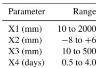
[image:4.612.75.259.268.500.2]Table 2.Ranges of GR4J parameters used for parameter calibration (Demirel et al., 2013).
Parameter Range
X1 (mm) 10 to 2000
X2 (mm) −8 to+6
X3 (mm) 10 to 500
X4 (days) 0.5 to 4.0
(NSE) and the water balance error (WBE) together:
OBJ=(1−NSE)+5|ln(1+WBE)|2.5, (2) NSE=1−
PN
i=1 Qobs,i−Qsim,i 2
PN
i=1 Qobs,i−Qobs
2 , (3)
WBE= PN
i=1 Qobs,i−Qsim,i
PN i=1Qobs,i
, (4)
whereQobs andQsimare the observed and simulated flows respectively, Qobsis the arithmetic mean of Qobs, andN is the total number of flow observations. The best parameter set for each study catchment was obtained from minimisation of the OBJ using the Monte Carlo simulations described below. To determine sufficient runs for the random simulations, we calibrated GR4J parameters using the shuffled complex evolution (SCE) algorithm (Duan et al., 1992) for one catch-ment with moderate input–output consistency with the pa-rameter range given in Table 2 by Demirel et al. (2013). Then, the total number of random simulations was iteratively determined by adjusting the number of runs until the min-imum OBJ of the random simulations became adequately close to the OBJ value from the SCE algorithm. We found that approximately 20 000 runs could provide the minimum OBJ value equivalent to that from the SCE algorithm. Sub-sequently, GR4J was calibrated by 20 000 runs of the Monte Carlo simulations for all 45 catchments, and the parameter sets with the minimum OBJ values were taken for runoff pre-dictions. In addition, we sorted the 20 000 parameter sets in terms of corresponding OBJ values in ascending order, and the first 50 sets (0.25 % of the total samples) were taken to measure the degree of equifinality. We measured the equifi-nality simply by the prediction area between 2.5 and 97.5 % boundaries of runoff simulations given by the collected 50 parameter sets. This prediction area was later compared to that from the FDC calibration under the same Monte Carlo framework. Note that we estimated the prediction area to comparatively evaluate the degree of equifinality between the hydrograph and the FDC calibrations under the same sam-pling size and the same acceptance rate for all the catch-ments. For more sophisticated and reliable uncertainty es-timation other methods are available, such as the gener-alised likelihood uncertainty estimation (GLUE; Beven and Bingley, 1992), the Bayesian total error analysis (BATEA;
Kavetski et al., 2006), and the differential evolution adaptive Metropolis (DREAM; Vrugt and Ter Braak, 2011).
For the hydrograph calibration, the 9-year streamflow data were divided into two parts for calibration (2011–2015) and for validity check (2007–2010), respectively. A 2-year warm-up period was used for initialising all runoff simulations in this study.
3.4 Model calibration against the regional FDC for ungauged catchments
Each catchment was treated ungauged for the compara-tive evaluation of RFDC_cal in the leave-one-out cross-validation (LOOCV) mode. For regionalising empirical FDC, the geostatistical method recently proposed by Pugliese et al. (2014) was used. Pugliese et al. (2014) em-ployed the top-kriging method (Skøien et al., 2006) to spa-tially interpolate the total negative deviation (TND), which is defined as the area between the mean annual flow and below-average flows in a normalised FDC. The top-kriging weights that interpolate TND values were taken as weights to esti-mate flow quantiles of ungauged catchments from empirical FDC of surrounding gauged catchments. The FDC of an un-gauged catchment in Pugliese et al. (2014) is estimated from normalised FDC of surrounding gauged catchments as
ˆ
8 (w0, p)= ˆφ (w0, p)·Q (w0) , (5) ˆ
φ (w0, p)= n X
i=1
λi·φi(wi, p) p(0,1), (6)
where 8 (wˆ 0, p) is the estimated quantile flow (m3s−1) at an exceedance probability p (unitless) for an ungauged catchmentw0,φ (wˆ 0, p)is the estimated normalised quan-tile flow (unitless),Q (w0) is the annual mean streamflow (m3s−1)of the ungauged catchment, andφ
i(wi, p)andλi are normalised quantile flows (unitless) and corresponding top-kriging weights (unitless) of gauged catchmentwi, re-spectively. The unknown mean annual flow of an ungauged catchment,Q (w0), can be estimated with a rescaled mean annual precipitation defined as
MAP∗=3.171×10⁻⁵·MAP·A, (7) where MAP∗ is the rescaled mean annual precipitation (m3s−1), MAP is mean annual precipitation (mm yr−1), and A is the area (km2) of the ungauged catchment, and the constant 3.171×10⁻⁵ converts the units of MAP∗ from mm yr−1km2to m3s−1.
or partly lost. The geostatistical method, on the other hand, treats all flow quantiles as a single object; thereby, features in an FDC continuum can be preserved. It showed promising performance to reproduce empirical FDC only using topo-logical proximity between catchments. More details on the geostatistical method can be found in Pugliese et al. (2014).
For regionalising empirical FDC of the 45 catchments, we followed the same procedure of Pugliese et al. (2014). We obtained top-kriging weights (λi) by the geostatistical in-terpolation of TND values from observed FDC for the cal-ibration period (2011–2015). Then, the top-kriging weights were used to interpolate empirical flow quantiles. The num-ber of neighbours for the TND interpolation was iteratively determined as five, at which level additional neighbouring TND are unlikely to bring better agreement between the es-timated and observed TND. In other words, normalised flow quantiles of five catchments surrounding the target ungauged catchment were interpolated with the top-kriging weights. Then, MAP∗ of the target ungauged catchment was multi-plied. We predicted flow quantiles at 103 exceedance proba-bilities (pof 0.001, 0.005, 99 points between 0.01 and 0.99 at an interval of 0.01, 0.995, and 0.999) for rainfall–runoff modelling against regional FDC (i.e. RFDC_cal).
For runoff prediction in ungauged catchments, the GR4J parameters were identified by the same Monte Carlo sam-pling but towards minimisation of OBJ value between the re-gional and the modelled flow quantiles at the 103 exceedance probabilities. The best parameter set, which provided the minimum OBJ value, was taken as the best behavioural set of RFDC_cal for each catchment.
3.5 Proximity-based parameter regionalisation for ungauged catchments
We selected the proximity-based parameter transfer (referred to as “PROX_reg” hereafter) to comparatively evaluate pre-dictive performance of RFDC_cal. The parameter regionali-sation has three classical categories: (a) proximity-based pa-rameter transfer (i.e. PROX_reg; e.g. Oudin et al., 2008); (b) similarity-based parameter transfer (e.g. McIntyre et al., 2005); and (c) regression between parameters and physi-cal properties of gauged catchments (e.g. Kim and Kalu-arachchi, 2008). A comprehensive review on the param-eter regionalisation in Parajka et al. (2013) reported that PROX_reg has competitive performance under humid cli-mate with low-complexity models relative to the other cat-egories. Based on modelling conditions in this study (semi-humid climate and four parameters), we chose PROX_reg to evaluate RFDC_cal.
To predict runoff at the 45 catchments in the LOOCV mode, we transferred the behavioural parameter sets obtained from the hydrograph calibration of the five donor catch-ments used for the FDC regionalisation. In other words, we used the same donor catchments for FDC regionalisa-tion and PROX_reg. This allowed us to have consistency
in transferring hydrological information from gauged to un-gauged catchments between RFDC_cal and PROX_reg. Us-ing the best behavioural parameter sets of the five donor catchments, we generated five runoff time series and took the arithmetic averages of them to represent runoff predic-tions by PROX_reg.
3.6 Performance evaluation
We used multiple performance metrics to evaluate predic-tive performance of all modelling approaches applied in this study. Predictive performance of each modelling approach was graphically evaluated using box plots of the performance metrics of the 45 catchments. In addition, we performed several pairedt tests to check the statistical significance of performance differences between the modelling approaches. What follows is the description of the performance metrics.
To measure high- and low-flow reproducibility, we chose two traditional performance metrics: (1) the NSE between observed and predicted flows (Eq. 2b) and (2) the NSE of log-transformed flows (LNSE) respectively. LNSE is calculated as
LNSE=1− PN
i=1 ln Qobs,i−ln Qsim,i2 PN
i=1 ln Qobs,i−ln(Qobs)
2 . (8)
Although NSE and LNSE are frequently used for perfor-mance evaluation, they may be sensitive to errors in flow observations (Westerberg et al., 2011). Hence, we addition-ally selected three typical flow metrics that embed dynamic flow variation in a compact manner: the runoff ratio (RQP), the baseflow index (IBF), and the rising limb density (DRL). RQP,IBF, andDRLare proxies of aridity and water-holding capacity, contribution of the baseflow to flow variations, and flashiness of catchment behaviours, respectively. They are defined as the ratio of runoff to precipitation, the ratio of baseflow to total runoff, and the inverse of average time to peak (d−1)as
RQP= Q
P, (9)
IBF= XT
t=1 QB,t
Qt
, (10)
DRL= NRL
TR
, (11)
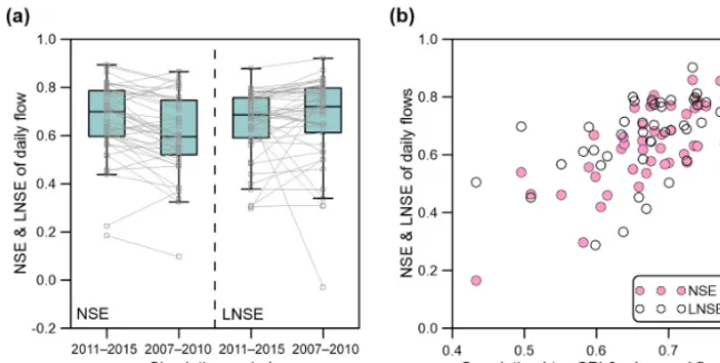
sub-Figure 3. (a)Box plots of high flow (NSE) and low flow (LNSE) reproducibility of the behavioural parameters obtained from the hydrograph calibration at the 45 catchments.(b)The relationship between the input–output consistency and the model performance. The straight lines in the box plots connect the performance metrics for the calibration (2011–2015) and the validation periods (2007–2010) in each catchment.
tracting direct flowQD,t fromQt as
QD,t=c·QD,t−1+0.5·(1+c)·(Qt−Qt−1) , (12)
QB,t=Qt−QD,t, (13)
where c is the filter parameter, which was set to 0.925 (Brooks et al., 2011; Eckhardt, 2007).
Flow signature reproducibility of RFDC_cal and PROX_reg were evaluated by the relative absolute bias between modelled and observed signatures as
DFS=
|FSsim−FSobs| FSobs
, (14)
whereDFSis the relative absolute bias, FSsimis a flow signa-ture of the modelled flows, and FSobsis that of the observed flows.
4 Results
4.1 Hydrograph calibration and FDC regionalisation in gauged catchments
Figure 3a displays results of the parameter identification against the observed hydrographs (i.e. the hydrograph cali-bration). The 45 catchments had mean NSE and LNSE of 0.66 and 0.65 between the simulated and observed flows for the calibration period, respectively. The average NSE reduc-tion from the calibrareduc-tion to the validareduc-tion periods was 0.06 with a standard deviation of 0.10. The temporal transfer of the calibrated parameters did not decrease the mean LNSE value, while a wider LNSE range indicates that uncertainty of low-flow predictions may increase when temporally trans-ferring the calibrated parameters.
The predictive performance was closely related to the input–output consistency (Fig. 3b), which was measured by
the Pearson correlation coefficient between the CPI and the observed flows. A low input–output consistency implies that the rainfall–runoff data may include significant epistemic er-rors such as minimal flow responses to heavy rainfall or excessive response to tiny rainfall. If the model calibration compensates disinformation from such errors, the parameters would be forced to have biases. Figure 3b shows that consis-tency in input–output data is a critical factor affecting param-eter identification and thus performance. Perhaps screening catchments with low input–output consistency would provide better predictions in ungauged catchments. However, we did not consider it in the LOOCV for RFDC_cal and PROX_reg, since variation in input–output consistency would be a com-mon situation. Rather, reducing the number of gauged catch-ments lowers spatial proximity, and thus can cause biases for ungauged catchments too. Overall, 27 catchments and 33 catchments showed NSE and LNSE values greater than 0.6. We assumed that the hydrograph calibration under the Monte Carlo framework, which was assisted by the SCE optimisa-tion, was able to acceptably identify the behavioural param-eters under given data quality.
[image:7.612.136.460.67.230.2]Figure 4.1 : 1 scatter plot between the empirical flow quantiles and the flow quantiles predicted by the top-kriging FDC regionalisation method.
0.7. This result is consistent with a finding of Pugliese et al. (2016) that performance of the geostatistical method was sensitive to river gauging density. Transferring flow quantiles from remote catchments may not sufficiently capture func-tional similarity between donor and receiver catchments. In spite of the minor shortcomings, the geostatistical FDC re-gionalisation was deemed acceptable based on the high NSE and LNSE of flow quantiles. Topological proximity was gen-erally a good predictor of flow quantiles for the study catch-ments.
4.2 Comparing hydrograph predictability between RFDC_cal and PROX_reg
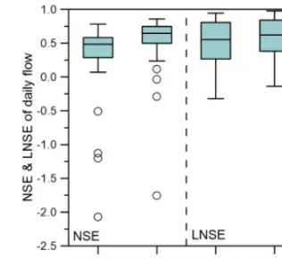
Figure 5 compares the box plots of NSE and LNSE val-ues between RFDC_cal and PROX_reg. PROX_reg gener-ally outperforms RFDC_cal in predicting both high and low flows, suggesting that transferring parameters identified by observed hydrographs would be a better choice than a local calibration against predicted FDC. The differences between NSE values of PROX_reg and RFDC_cal have an average of 0.22 with a standard deviation of 0.34. Only eight catchments showed higher NSE with RFDC_cal. These higher NSE val-ues of PROX_reg imply that PROX_reg is preferable when high-flow predictability is needed such as for flood analyses. In the case of LNSE, PROX_reg still had a higher median than RFDC_cal (0.53 and 0.62 for RFDC_cal and PROX_reg respectively). In 25 catchments, PROX_reg provided LNSE values greater than those of RFDC_cal.
[image:8.612.349.507.67.212.2]The low performance of RFDC_cal was also found in the comparative assessment of Zhang et al. (2015), which eval-uated RFDC_cal for 228 Australian catchments using the same GR4J model. Zhang et al. (2015) found that RFDC_cal was inferior to PROX_reg in the Australian catchments, be-cause the FDC calibration poorly reproduced temporal flow variations relative to the hydrograph calibration. This study
Figure 5.Box plots of NSE and LNSE values between the observed and the predicted hydrographs by RFDC_cal and PROX_reg for the 45 catchments under the cross-validation mode.
confirms the difficulty of capturing dynamic catchment be-haviours with FDC containing no flow timing information.
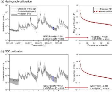
Figure 6.The observed and predicted hydrographs, the prediction areas, and the observed and predicted FDC given by(a)the hydrograph calibration and(b)the FDC calibration for Namgang Dam (Catchment 2 in Fig. 1).
Figure 7.The input–output consistency vs. equifinality increased by replacing the hydrograph calibration with the FDC calibration. The equifinality ratio is defined as the ratio between the prediction areas of the 50 behavioural parameters gained from the FDC cali-bration and the hydrograph calicali-bration.
equifinality problem embedded in RFDC_cal could be more significant than that in PROX_reg.
4.3 Comparing flow signature predictability between RFDC_cal and PROX_reg
coef-Figure 8. Flow signature reproducibility comparison between
RFDC_cal and PROX_reg in terms of RQP (a), IBF (b), and
DRL(c).
ficient of variance (CV) of direct runoff was 5.86 for 2007– 2015, which is approximately 3.5 times as high as the CV of the baseflow.
On the other hand, RFDC_cal was less able to repro-duceDRLthan PROX_reg. This highlights the weakness of RFDC_cal in which only flow magnitudes were used for identifying model parameters. PROX_reg showed better per-formance in predictingDRLthan did RFDC_cal. Flow tim-ing information gained from the observed hydrographs could be preserved, even after behavioural parameters were trans-ferred to ungauged catchments. Overall, PROX_reg seems to be better than RFDC_cal to predict the three flow signatures together.
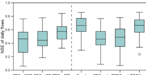
The box plots in Fig. 9 provide an indication thatDRLis likely to supplement the FDC calibration and thus improve RFDC_cal. From the collection of 50 behavioural parameter sets given by the FDC calibration, we chose the parameter set providing the lowest bias for each flow signature as the best behavioural sets, and simulated runoff again for all catch-ments. The high-flow predictability was fairly improved by additional constraining withDRL, suggesting that flow met-rics associated with flow timing make up for the weakness of the FDC calibration. Additional constraining with RQPand IBFdid not bring appreciable improvement in the FDC cal-ibration. However, PROX_reg was still better than the addi-tional constraining withDRL, indicating that a further study is needed for better constraining rainfall–runoff models using FDC together with additional flow metrics.
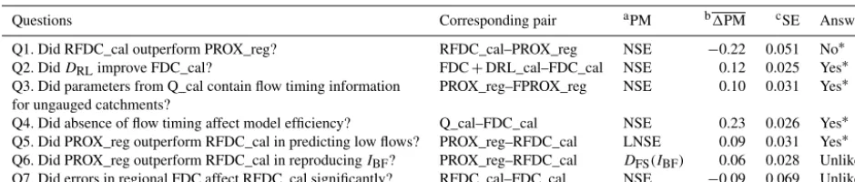
4.4 Pairedttests between the modelling approaches For comparative evaluation in this study, we produced sev-eral runoff prediction sets using multiple rainfall modelling approaches. First, we calibrated GR4J against the observed hydrographs (referred to as Q_cal), and transferred the be-havioural parameters to ungauged catchments in the LOOCV mode (PROX_reg). We constrained GR4J with the regional
FDC (RFDC_cal). To evaluate equifinality, we recalibrated the GR4J parameters against the observed FDC (referred to as FDC_cal). Additionally, we constrained the model with observed FDC plus the flow signatures, and signifi-cant performance improvement was found with DRL (re-ferred to as FDC+DRL_cal). A paired t test using the performance metrics (NSE, LNSE, orDFS)between these modelling approaches can answer various questions be-yond the graphical evaluations with box plots. For paired t tests, we added one more case of transferring parameters gained from FDC_cal to ungauged catchments (referred to as FPROX_reg). FPROX_reg transfers behavioural parameters with no flow timing information from gauged to ungauged catchments. The mean NSE of FPROX_reg was 0.44 with a standard deviation of 0.49.
A primary hypothesis of this study was that RFDC_cal could outperform PROX_reg. This question can be addressed by looking at the NSE differences between RFDC_cal and PROX_reg. The mean NSE difference between them was
−0.22 and the standard error was 0.051, providing an evalu-ation that the NSE differences were less than zero at a 95 % confidence level. The pairedttest did not lend support to the hypothesis (i.e. PROX_reg outperformed RFDC_cal signifi-cantly). However, we can assume thatDRLcan improve the predictive performance of FDC_cal. The mean NSE differ-ence between FDC+DRL_cal and FDC_cal was 0.12 and the standard error was 0.025, confirming the significance at a 95 % confidence level.
[image:10.612.47.287.67.212.2]Table 3.Results of the pairedttests for potential questions on rainfall–runoff modelling in ungauged catchments.
Questions Corresponding pair aPM b1PM cSE Answer
Q1. Did RFDC_cal outperform PROX_reg? RFDC_cal–PROX_reg NSE −0.22 0.051 No∗ Q2. DidDRLimprove FDC_cal? FDC+DRL_cal–FDC_cal NSE 0.12 0.025 Yes∗ Q3. Did parameters from Q_cal contain flow timing information PROX_reg–FPROX_reg NSE 0.10 0.031 Yes∗ for ungauged catchments?
Q4. Did absence of flow timing affect model efficiency? Q_cal–FDC_cal NSE 0.23 0.026 Yes∗ Q5. Did PROX_reg outperform RFDC_cal in predicting low flows? PROX_reg–RFDC_cal LNSE 0.09 0.031 Yes∗ Q6. Did PROX_reg outperform RFDC_cal in reproducingIBF? PROX_reg–RFDC_cal DFS(IBF) 0.06 0.028 Unlikely Q7. Did errors in regional FDC affect RFDC_cal significantly? RFDC_cal–FDC_cal NSE −0.09 0.069 Unlikely
aPerformance metric used forttest.bMean PM difference between the corresponding pair.cStandard error of1PM.∗
1PM is significantly different from zero. The significance was evaluated at 95 % confidence levels.
5 Discussion and conclusions
5.1 RFDC_cal for rainfall–runoff modelling in ungauged catchments
The use of regional FDC as a single calibration criterion ap-pears to be a good choice for searching behavioural param-eters in ungauged sites. As discussed earlier, the FDC is a compact representation of runoff variability at all timescales, and thus able to embed multiple hydrological features in catchment dynamics (Blöschl et al., 2013). A pilot study of Yokoo and Sivapalan (2011) discovered that the upper part of an FDC is controlled by interaction between extreme rain-fall and fast runoff, while the lower part is governed by base-flow recession behaviour during dry periods. The middle part connecting the upper and the lower parts is related to the mean withyear flow variations, which is controlled by in-teractions between water availability, energy, and water stor-age (Yaeger et al., 2012; Yokoo and Sivapalan, 2011). It is well documented that hydro-climatological processes within a catchment are reflected in the FDC (e.g. Cheng et al., 2012; Ye et al., 2012; Coopersmith et al., 2012; Yaeger et al., 2012; Botter et al., 2008), and therefore the model parameters iden-tified solely by a regional FDC are expected to provide reli-able predictions in ungauged catchments (e.g. Westerberg et al., 2014; Yu and Yang, 2000).
The comparative evaluation in this study provides another expected result, that the FDC calibration is able to repro-duce the FDC itself, but it insufficiently captures functional responses of catchments due to the absence of flow timing in-formation. A hydrograph is the most complete flow signature embedding numerous processes interacting within a catch-ment (Blöschl et al., 2013), being more informative than an FDC. Since any simplification of a hydrograph, including the FDC, loses some amount of flow information, it is no surprise that the FDC calibration worsens the equifinality. This study emphasises that the absence of flow timing in RFDC_cal may cause larger prediction errors than regionalised param-eters gained from observed hydrographs. The paired t test between PROX_reg and FPROX_reg highlights that region-alised parameters gained from observed hydrographs were
likely to contain intangible flow timing information even for ungauged catchments. The flow timing information implic-itly transferred to ungauged catchments is a major difference between PROX_reg and RFDC_cal. The errors introduced by the FDC regionalisation were not significant due to the high performance of the geostatistical method in this study.
Because the hydrograph calibration can compensate for the errors in input–output data, one may convert the hy-drograph into the FDC to avoid effects of disinformation on rainfall–runoff modelling. However, in this case, valu-able flow timing information should be balanced in trade-off. For RFDC_cal in this study, we began with converting the observed hydrographs into the flow quantiles to region-alise them; thus, the flow timing information was initially lost. As shown, the performance of RFDC_cal was gener-ally lower than that of PROX_reg. Therefore, when condens-ing observed hydrographs into flow signatures, preservcondens-ing all available flow information in the hydrograph would be key for a successful rainfall–runoff modelling. This study shows that using only regionalised FDC could lead to less reliable rainfall–runoff modelling in ungauged catchments than regionalised parameters. An FDC is unlikely to preserve all flow information in a hydrograph necessary for rainfall– runoff modelling.
5.2 Suggestions for improving RFDC_cal
Figure 9. Predictive performance of the FDC calibrations
ad-ditionally conditioned by RQP (FDC+RQP), IBF (FDC+IBF),
andDRL(FDC+DRL) in comparison to the other modelling
ap-proaches. Q_cal and FDC_cal refer to the hydrograph and the FDC calibration in gauged catchments respectively. Thirty-eight catch-ments with positive NSE for all the modelling approaches were used in the box plots.
An alternative method of RFDC_cal is to directly region-alise hydrographs to ungauged catchments (e.g. Viglione et al., 2013). In data-rich regions, topological proximity could better capture spatial variation of daily flows than rainfall– runoff modelling with regionalised parameters (Viglione et al., 2013). Although a dynamic model may be required for regionalising observed daily flows at an expensive computa-tional cost, flow timing information would be contained in re-gionalised hydrographs. The parameter identification against the regional hydrographs may become a better approach than RFDC_cal and/or other signature-based calibrations. 5.3 Limitations and future research directions
There are caveats in our comparative evaluation. First, un-certainty in input–output data was not considered in our as-sessment. McMillan et al. (2012) reported typical ranges of relative errors in discharge data as 10–20 % for medium to high flow and 50–100 % for low flows. We assumed that quality of the discharge data was adequate. However, other methods objectively considering uncertainty could better es-timate model performance and the equifinality (e.g. Wester-berg et al., 2011, 2014). Second, we used a conceptual runoff model with a fixed structure for all the catchments. Uncer-tainty from the model structure would vary across the study catchments; nevertheless, the structural uncertainty was not measured here. Our comparative assessment was based on the basic premise that modelling conditions should be fixed for all study catchments. Third, we compared RFDC_cal and PROX_reg in a region with sufficient data lengths and qual-ity at gauged catchments. The lessons from this study may not be expandable to ungauged catchments under poor data availability. Finally, though the proximity-based parameter regionalisation was good for the South Korean catchments, comparison between RFDC_cal and other regionalisation
methods, such as the regional calibration and the similarity-based parameter transfer, may provide beneficial information for rainfall–runoff modelling in ungauged catchments. Com-parative assessment between RFDC_cal and other parameter regionalisation using more sample catchments under diverse climates will provide more meaningful lessons.
We can no longer hypothesise that the parameters gained against regionalised FDC would perform sufficiently, be-cause an FDC contains less information than a hydrograph (i.e. the absence of flow timing). For improving RFDC_cal, we suggest supplementing RFDC_cal with flow signatures in temporal dimensions. Then, the question of how to make flow signatures more informative than (or equally informa-tive to) hydrographs should be addressed. This may be im-possible only using flow signatures originating from hydro-graphs (e.g. mean annual flow, baseflow index, recession rates, FDC). Combinations of those signatures are unlikely to be more informative than their origins (i.e. hydrographs), though it depends on how much disinformation is present in the observed flows. Future research topics could include find-ing new signatures that supplement hydrographs, and how to combine them with existing flow signatures for rainfall– runoff modelling in ungauged catchments.
5.4 Conclusions
While rainfall–runoff modelling against regional FDC ap-peared a good approach for prediction in ungauged catch-ments, this study highlights its weakness in the absence of flow timing information, which may cause poorer predictive performance than the simple proximity-based parameter re-gionalisation. The following conclusions are worth empha-sising.
For ungauged catchments in South Korea, where spa-tial proximity well captured functional similarity between gauged catchments, the model calibration against regional FDC is unlikely to outperform the conventional proximity-based parameter transfer for daily runoff prediction. The ab-sence of flow timing information in regional FDC seems to cause a substantial equifinality problem in the parameter identification process and thus lower predictability.
The model parameters gained from observed hydrographs contain flow timing information even for ungauged catch-ments. This intangible flow timing information should be dis-carded if one calibrates a rainfall–runoff model against re-gional FDC. This information loss may reduce predictability in ungauged catchments significantly.
To improve the calibration against regional FDC, flow metrics in temporal dimensions, such as the rising limb den-sity, need to be included as additional constraints. As an alter-native approach, if river gauging density is high, regionalised hydrographs preserving flow timing information can be used for local calibrations at ungauged catchments.
observed hydrographs. How to combine them with existing information will be a future research topic for rainfall–runoff modelling in ungauged catchments.
Data availability. Data required to reproduce the modelling results are available upon request from the authors ([email protected], [email protected]).
Competing interests. The authors declare that they have no conflict of interest.
Acknowledgements. This study was supported by the APEC
Climate Center. We send special thanks to Yoe-min Jeong and Hyung-Il Eum for the PRISM data sets. We greatly appreciate constructive comments and suggestions from the reviewers that significantly improved the paper.
Edited by: Fabrizio Fenicia
Reviewed by: two anonymous referees
References
Atieh, M., Taylor, G., Sttar, A. M. A., and Gharadaghi, B.: Predic-tion of flow duraPredic-tion curves for ungauged basins, J. Hydrol., 545, 383–394, 2017.
Bae, D.-H., Jung, I.-W., and Chang, H: Long-term trend of precip-itation and runoff in Korean river basins, Hydrol. Process., 22, 2644–2656, 2008.
Bárdossy, A.: Calibration of hydrological model parameters for ungauged catchments, Hydrol. Earth Syst. Sci., 11, 703–710, https://doi.org/10.5194/hess-11-703-2007, 2007.
Beven, K. J.: Prophecy, reality and uncertainty in distributed hydro-logical modelling, Adv. Water Resour., 16, 41–51, 1993. Beven, K. J.: A manifesto for the equifanality thesis, J. Hydrol., 320,
18–36, 2006.
Beven, K. J. and Bingley, A.: The future of distributed models. Model calibration and uncertainty prediction, Hydrol. Process., 6, 279–298, 1992.
Blazkova, S. and Beven, K.: A limits of acceptability approach to model evaluation and uncertainty estimation in flood fre-quency estimation by continuous simulation: Skalka catch-ment, Czech Republic, Water Resour. Res., 45, W00b16, https://doi.org/10.1029/2007wr006726, 2009.
Blöschl, G., Sivapalan, M., Wagener, T., Viglione, A., and Savenije, H.: Runoff Prediction in Ungauged Basins, Simthesis across Pro-cesses, Places, and Scales, Cambridge University Press, New York, USA, 2013.
Botter, G., Porporato, A., Rodriguez-Iturbe, I., and Rinaldo, A.: Basin-scale soil moisture dynamics and the probabilistic char-acterization of carrier hydrologic flows: Slow, leaching-prone components of the hydrologic response, Water Resour. Res., 43, W02417, https://doi.org/10.1029/2006WR005043, 2007. Botter, G., Zanardo, S., Porporato, A., Rodriguez-Iturbe, I.,
and Rinaldo, A.: Ecohydrological model of flow duration
curves and annual minima, Water Resour. Res., 44, W08418, https://doi.org/10.1029/2008WR006814, 2008.
Brooks, P. D., Troch, P. A., Durcik, M., Gallo, E., and Schlegel, M.: Quantifying regional-scale ecosystem response to changes in precipitation: Not all rain is created equal, Water Resour. Res., 47, W00J08, https://doi.org/10.1029/2010WR009762, 2011. Cheng, L., Yaeger, M., Viglione, A., Coopersmith, E., Ye, S.,
and Sivapalan, M.: Exploring the physical controls of re-gional patterns of flow duration curves – Part 1: Insights from statistical analyses, Hydrol. Earth Syst. Sci., 16, 4435–4446, https://doi.org/10.5194/hess-16-4435-2012, 2012.
Coopersmith, E., Yaeger, M. A., Ye, S., Cheng, L., and Sivapalan, M.: Exploring the physical controls of regional patterns of flow duration curves – Part 3: A catchment classification system based on regime curve indicators, Hydrol. Earth Syst. Sci., 16, 4467– 4482, https://doi.org/10.5194/hess-16-4467-2012, 2012. Daly, C., Halbleib, M., Smith, J. I., Gibson, W. P., Doggett, M. K.,
Taylor, G. H., Curtis, J., and Pasteris, P. P.: Physiographically sensitive mapping of climatological temperature and precipita-tion across the conterminous United States, Int. J. Climatol., 28, 2031–2064, https://doi.org/10.1002/joc.1688, 2008.
Demirel, M. C., Booiji, M. J., and Hoekstra, A. Y.: Effect of differ-ent uncertainty sources on the skill of 10 day ensemble low flow forecasts for two hydrological models, Water Resour. Res., 49, 4035–4053, https://doi.org/10.1002/wrcr.20294, 2013.
Duan, Q., Sorooshian, S., and Gupta, V. K.: Effective and efficient global optimisation for conceptual rainfall–runoff models, Water Resour. Res., 28, 1015–1031, 1992.
Dunn, S. M. and Lilly, A.: Investigating the relationship between a soils classification and the spatial parameters of a conceptual catchment scale hydrological model, J. Hydrol., 252, 157–173, https://doi.org/10.1016/S0022-1694(01)00462-0, 2001.
Eckhardt, K.: A comparison of baseflow indices,
which were calculated with seven different
base-flow separation methods, J. Hydrol., 352, 168–173,
https://doi.org/10.1016/j.jhydrol.2008.01.005, 2007.
Hingray, B., Schaefli, B., Mezghani, A., and Hamdi, Y.: Signature-based model calibration for hydrological prediction in mesoscale Alpine catchments, Hydrolog. Sci. J., 55, 1002–1016, https://doi.org/10.1080/02626667.2010.505572, 2010.
Hrachowitz, M., Savenije, H. H. G., Blöschl, G., McDonnell, J. J., Sivapalan, M., Pomeroy, J. W., Arheimer, B., Blume, T., Clark, M. P., Ehret, U., Fenicia, F., Freer, J. E., Gelfan, A., Gupta, H. V., Hughes, D. A., Hut, R. W., Montanari, A., Pande, S., Tetzlaff, D., Troch, P. A., Uhlenbrook, S., Wagener, T., Winsemius, H. C., Woods, R. A., Zehe, E., and Cudennec, C.: A decade of Predic-tions in Ungauged Basins (PUB) – a review, Hydrolog. Sci. J., 58, 1198–1255, https://doi.org/10.1080/02626667.2013.803183, 2013.
Jung, Y. and Eum, H.-I.: Application of a statistical interpolation method to correct extreme values in high-resolution gridded cli-mate variables, J. Clim. Chang. Res., 6, 331–334, 2015. Kavetski, D., Fnicia, F., and Clark, M.: Impact of temporal
data resolution on parameter inference and model identifica-tion in conceptual hydrological modeling: Insights from an experimental catchment, Water Resour. Res., 47, W05501, https://doi.org/10.1029/2010WR009525, 2011.
Kavetski, D., Kuczera, G., and Franks, S. W.: Bayesian
analysis of input uncertainty in hydrological
mod-eling: 1. Theory, Water Resour. Res., 42, W03407,
https://doi.org/10.1029/2005WR004368, 2006.
Kim, D. and Kaluarachchi, J.: Predicting streamflows in snowmelt-driven watersheds using the flow duration curve method, Hydrol. Earth Syst. Sci., 18, 1679–1693, https://doi.org/10.5194/hess-18-1679-2014, 2014.
Kim, U. and Kaluarachchi, J. J.: Application of parameter estima-tion and regionalizaestima-tion methodologies to ungauged basins of the Upper Blue Nile River Basin, Ethiopia, J. Hydrol., 362, 39–56, https://doi.org/10.1016/j.jhydrol.2008.08.016, 2008.
Korea Meteorological Administration: Climatological normals of Korea (1981–2010), Publ. 11-1360000-000077-14, 678 pp., available at: http://www.kma.go.kr/down/Climatological_2010. pdf (last access: 16 January 2017), 2011.
McIntyre, N., Lee, H., Wheater, H., Young, A., and
Wagener, T.: Ensemble predictions of runoff in
un-gauged catchments, Water Resour. Res., 41., W12434,
https://doi.org/10.1029/2005WR004289, 2005.
McMillan, H., Krueger, T., and Freer, J.: Benchmarking observa-tional uncertainties for hydrology: rainfall, river discharge, and water quality, Hydrol. Process., 26, 4078–4111, 2012.
Mohamoud, Y. M.: Prediction of daily flow duration curves and streamflow for ungauged catchments using regional flow dura-tion curves, Hydrolog. Sci. J., 53, 706–724, 2008.
Oudin, L., Hervieu, F., Michel, C., Perrin, C., Andréassian, V., An-ctil, F., and Loumagne, C.: Which potential evapotranspiration input for a lumped rainfall-runoff model? Part 2 – Towards a sim-ple and efficient potential evapotranspiration model for rainfall-runoff modelling, J. Hydrol., 303, 290–306, 2005.
Oudin, L., Andréassian, V., Perrin, C., Michel, C., and Le Moine, N.: Spatial proximity, physical similarity, regression and un-gaged catchments: a comparison between of regionalization ap-proaches based on 913 French catchments, Water Resour. Res., 44, W03413, https://doi.org/10.1029/2007WR006240, 2008. Parajka, J., Blöschl, G., and Merz, R.: Regional calibration of
catch-ment models: potential for ungauged catchcatch-ments, Water Resour. Res., 43, W06406, https://doi.org/10.1029/2006WR005271, 2007.
Parajka, J., Viglione, A., Rogger, M., Salinas, J. L., Sivapalan, M., and Blöschl, G.: Comparative assessment of predictions in ungauged basins – Part 1: Runoff-hydrograph studies, Hydrol. Earth Syst. Sci., 17, 1783–1795, https://doi.org/10.5194/hess-17-1783-2013, 2013.
Perrin, C., Michel, C., and Andréassian, V.: Improvement of a parsi-monious model for streamflow simulation, J. Hydrol., 279, 275– 289, 2003.
Pfannerstill, M., Guse, B., and Fohrer N.: Smart low flow signa-ture metrics for an improved overall performance evaluation of hydrological models, J. Hydrol., 510, 447–458, 2014.
Pugliese, A., Castellarin, A., and Brath, A.: Geostatistical predic-tion of flow-durapredic-tion curves in an index-flow framework, Hydrol. Earth Syst. Sci., 18, 3801–3816, https://doi.org/10.5194/hess-18-3801-2014, 2014.
Pugliese, A., Farmer, W. H., Castellarin, A., Archfield, S. A., and Vogel, R. M.: Regional flow duration curves: Geostatistical tech-niques versus multivariate regression, Adv. Water Resour., 96, 11–22, 2016.
Rhee, J. and Cho, J.: Future changes in drought characteristics: re-gional analysis for South Korea under CMIP5 projections, J. Hy-drometeorol., 17, 437–450, 2016.
Sadegh, M., Vrugt, J. A., Gupta, H. V., and Xu, C.: The soil water characteristics as new class of closed-form parametric expres-sions for the flow duration curve, J. Hydrol., 535, 438–456, 2016. Shafii, M. and Tolson, B. A.: Optimizing hydrological con-sistency by incorporating hydrological signatures into model calibration objectives, Water Resour. Res., 51, 3796–3814, https://doi.org/10.1002/2014WR016520, 2015.
Shu, C. and Ouarda, T. B. M. J.: Improved methods for daily streamflow estimates at ungauged sites, Water Resour. Res., 48, W02523, https://doi.org/10.1029/2011WR011501, 2012. Skøien, J. O., Merz, R., and Blöschl, G.: Top-kriging –
geostatis-tics on stream networks, Hydrol. Earth Syst. Sci., 10, 277–287, https://doi.org/10.5194/hess-10-277-2006, 2006.
Smakhtin, V. P. and Masse, B.: Continuous daily hydrograph sim-ulation using duration curves of a precipitation index, Hydrol. Process., 14, 1083–1100, 2000.
Smakhtin, V. Y., Hughes, D. A., and Creuse-Naudine, E.: Regional-ization of daily flow characteristics in part of the Eastern Cape, South Africa, Hydrolog. Sci. J., 42, 919–936, 1997.
Sugawara, M.: Automatic calibration of the tank
model, Hydrological Sciences Bulletin, 24, 375–388,
https://doi.org/10.1080/02626667909491876, 1979.
Viglione, A., Parajka, J., Rogger, M., Salinas, J. L., Laaha, G., Sivapalan, M., and Blöschl, G.: Comparative assessment of predictions in ungauged basins – Part 3: Runoff signa-tures in Austria, Hydrol. Earth Syst. Sci., 17, 2263–2279, https://doi.org/10.5194/hess-17-2263-2013, 2013.
Vogel, R. M. and Fennessey, N. M.: Flow duration curves. I: New interpretation and confidence intervals, J. Water Res. Plan. Man., 120, 485–504, 1994.
Vrugt, J. A. and Ter Braak, C. J. F.: DREAM(D): an adaptive
Markov Chain Monte Carlo simulation algorithm to solve dis-crete, noncontinuous, and combinatorial posterior parameter es-timation problems, Hydrol. Earth Syst. Sci., 15, 3701–3713, https://doi.org/10.5194/hess-15-3701-2011, 2011.
Wagener, T. and Wheater, H. S.: Parameter estimation and region-alization for continuous rainfall-runoff models including uncer-tainty, J. Hydrol., 320, 132–154, 2006.
Walter, M. T., Brooks, E. S., McCool, D. K., King, L. G., Molnau, M., and Boll, J.: Process-based snowmelt modeling: does it re-quire more input data than temperature-index modeling?, J. Hy-drol., 300, 65–75, https://doi.org/10.1016/j.jhydrol.2004.05.002, 2005.
Westerberg, I. K. and McMillan, H. K.: Uncertainty in hydro-logical signatures, Hydrol. Earth Syst. Sci., 19, 3951–3968, https://doi.org/10.5194/hess-19-3951-2015, 2015.
hydrological models using flow-duration curves, Hydrol. Earth Syst. Sci., 15, 2205–2227, https://doi.org/10.5194/hess-15-2205-2011, 2011.
Westerberg, I. K., Gong, L., Beven, K. J., Seibert, J., Semedo, A., Xu, C.-Y., and Halldin, S.: Regional water balance modelling using flow-duration curves with observational
uncertainties, Hydrol. Earth Syst. Sci., 18, 2993–3013,
https://doi.org/10.5194/hess-18-2993-2014, 2014.
Westerberg, I. K., Wagener, T., Coxon, G., McMillan, H. K., Castellarin, A., Montanari, A., and Freer, J.: Un-certainty in hydrological signatures for gauged and un-gauged catchments, Water Resour. Res., 52, 1847–1865, https://doi.org/10.1002/2015WR017635, 2016.
Yadav, M., Wagener, T., and Gupta, H.: Regionalization of con-straints on expected watershed response behavior for improved predictions in ungauged basins, Adv. Water Resour., 30, 1756– 1774, 2007.
Yaeger, M., Coopersmith, E., Ye, S., Cheng, L., Viglione, A., and Sivapalan, M.: Exploring the physical controls of regional pat-terns of flow duration curves – Part 4: A synthesis of empirical analysis, process modeling and catchment classification, Hydrol. Earth Syst. Sci., 16, 4483–4498, https://doi.org/10.5194/hess-16-4483-2012, 2012.
Ye, S., Yaeger, M., Coopersmith, E., Cheng, L., and Sivapalan, M.: Exploring the physical controls of regional patterns of flow du-ration curves – Part 2: Role of seasonality, the regime curve, and associated process controls, Hydrol. Earth Syst. Sci., 16, 4447– 4465, https://doi.org/10.5194/hess-16-4447-2012, 2012.
Yilmaz, K. K., Gupta, H. V., and Wagener, T.: A process-based di-agnostic approach to model evaluation: Application to the NWS distributed hydrologic model, Water Resour. Res., 44, W09417, https://doi.org/10.1029/2007WR006716, 2008.
Yokoo, Y. and Sivapalan, M.: Towards reconstruction of the flow duration curve: development of a conceptual framework with a physical basis, Hydrol. Earth Syst. Sci., 15, 2805–2819, https://doi.org/10.5194/hess-15-2805-2011, 2011.
Yu, P.-S. and Yang, T.-C.: Using synthetic flow duration curves for rainfall–runoff model calibration at ungauged sites, Hy-drol. Process., 14, 117–133, https://doi.org/10.1002/(SICI)1099-1085(200001)14:1<117::AID-HYP914>3.0.CO;2-Q, 2000. Yu, P. S., Yang, T. C., and Wang, Y. C.: Uncertainty analysis of
regional flow duration curves, J. Water Res. Pl.-ASCE, 128, 424– 430, 2002.
Zhang, Y., Vaze, J., Chiew, F. H. S., and Li, M.: Comparing flow duration curve and rainfall-runoff modelling for predicting daily runoff in ungauged catchments, J. Hydrol., 525, 72–86, 2015. Zhang, Z., Wagener, T., Reed, P., and Bhushan, R.: