Acceptance Sampling Plans: Size Biased Lomax Model
R. Subba Rao
1, A. Naga Durgamamba
2,*, R.R.L. Kantam
31Shri Vishnu Engineering College for Women, Bhimavaram, 534202, Andhra Pradesh, India 2Raghu Institute of Technology, Dakamarri, Visakhapatnam, 531162, Andhra Pradesh, India
3Acharya Nagarjuna University, Guntur, 522510, Andhra Pradesh, India *Corresponding Author: [email protected]
Copyright © 2014 Horizon Research Publishing All rights reserved.
Abstract
A new probability model size biased Lomax is considered for a life time random variable. The problem of acceptance sampling when the life test is truncated at a pre-assigned time is discussed with a known shape parameter. For various acceptance numbers, confidence levels and values of the ratio of the fixed experimental time to the specified mean life, the minimum sample size necessary to assure the specified mean life time is evaluated. The operating characteristic functions of the sampling plans are derived. Producer’s risk is also discussed. A table for the ratio of true mean life to a specified mean life that ensure acceptance with a pre-assigned probability is provided. The results are given by an example.Keywords
Size Biased Lomax Model (SBLM), Operating Characteristic (O.C), Truncated Life Test, Sampling Plans1. Introduction
The probability density function (p.d.f) g(t) and cumulative distribution function(c.d.f) G(t) of Lomax(Pareto type II) model are respectively given by
(
1)
(t) 1 t ; 0, 0, 0
g α α t α σ
σ σ
− +
= + ≥
(1)
F(t) 1 1 t α;t 0,α 0,σ 0
σ
−
= − + ≥
(2)
where σ is the scale parameter and α is known as shape parameter.
The expected value and variances are
( )
( )
(
) (
)
2
; 1 2 ; 2
1 1 2
E t σ α and V t ασ α
α α α
= =
− − − (3)
The concept of weighted distribution, which was introduced by Rao(1965), has many applications in different areas of statistics such as survey sampling, reliability, bio-statistics etc,. Let X be a non-negative random variable
with a probability density function f(x;θ), where the natural parameter
θ
∈Ω
(Ω is the parameter space). The weight function w(x,β) is a non-negative function with the parameter β representing the sighting (recording) mechanism. The p.d.f of weighted distribution is(
; ,
)
(
, .
) ( )
(
)
;
,
w
w x
f x
f x
E w x
β
θ
θ β
β
=
(4)where E[w(x,β)] is the normalizing factor.
The random variable
X
wis called the weighted version of the random variable X and its distribution is called the weighted distribution with weight function w. When w(x,β) = X, in which caseX
∗=
X
w is called size biased version of X. The distributions ofX
∗ is called a size biased distribution with p.d.f.( )
( )
.
;
x f x
f
E x
θ
∗
=
(5)The p.d.f
'
f
∗'
is called the size biased or length biased version of f and the corresponding observational mechanism is called size biased sampling.Size biased sampling was introduced by Cox 1962(see Patil 2002). The two models weighted and size biased found various applications in biomedical area such as family history and disease, survival and intermediate events and latency period of AIDS due to blood transfusion (Gupta & Akman 1995). The size biased Lomax model has played a very important role in the socio-economic quantities such as city population sizes, stock price fluctuations, personal incomes, etc,. The p.d.f and c.d.f of size biased Lomax model are given by
(
1)
(
1)
(t) t 1 t ; 0, 1, 0
f α α α t α σ
σ σ σ
− +
−
= + ≥
(6)
F(t) 1 1 1 ; 0, 1
0
t t α t
α α σ σ σ − = − + + ≥ (7)
parameters m = 2 and n = α-1.
Acceptance sampling plans based on life tests are studied by many authors. Gamma distribution in acceptance sampling based on life tests derived by S.S. Gupta and P.A. Groll[3], R.R.L. Kantam and K. Rosaiah[5] proposed half logistic distribution in acceptance sampling based on life tests, R.R.L. Kantam et al.[6] developed acceptance sampling based on life tests: log-logistic model, K. Rosaiah
et al.[10] discussed Pareto distribution in acceptance sampling based on truncated life test, G. Srinivas Rao et al.[11] introduced acceptance sampling plans for Marshall-Olkin extended Lomax distribution. A.A. Addel-Ghaly et al.[1] discussed estimation of the parameters of Pareto distribution and reliability function using accelerated life testing with censoring, G. Kulldorff and K. Vannman[7] studied estimation of the location and scale parameters of a Pareto distribution by linear functions of order statistics, K. Vannman[13] introduced estimators based on order statistics from a Pareto distribution, Acceptance sampling with new life test objectives developed by M. Sobel and J.A. Tisschendrof[12].
Size biased Lomax model in acceptance sampling based on life tests received little attention. In the present paper the probability distribution of a life time random variable is considered as size biased Lomax model with a known shape parameter. The problem of finding the minimum sample size necessary to assure a certain mean life when the life test is terminated at a pre-assigned time t and when the observed number of failures does not exceed a given acceptance number is studied. The decision procedure is to accept a lot only if the specified mean life can be established with a pre-assigned high probability p*, which provides the protection to the consumer. The decision to accept the lot can take place only at the end of time t and if the number of failures does not exceed the given acceptance number c. The life test experiment gets terminated at the time at which (c+1)th failure is observed or at time t whichever is earlier. In the first case the decision t reject the lot.
In Section 2, we have obtained the minimum sample sizes necessary for various acceptance numbers-c, confidence levels-p* and ratios of the test time-t to the specified mean life σ0 using cumulative binomial probabilities and cumulative Poisson probabilities for size biased Lomax model with a known shape parameter α = 2,3,4. Section 3 deals with the operating characteristic and producer’s risk of the sampling plans, the results are observed for α = 2,3,4. Due to the space constraints the results are presented in this paper only for α = 2. The use of the numerical table through an illustration is described and is compared with similar plans constructed for some other model that are presented in Section 4.
2. The Sampling Plan
Acceptance sampling plans is helpful to reduce the time
and cost when the product is submitted for inspection. Quality control personnel can take decisions about quality of the product using sampling results instead of inspecting the whole lot. If the good lot is rejected on the basis of sample results this type of error is called type I error, while the good lot is not accepted by the consumer, this type of error is called type II error. Probability of type I error is called producer’s risk and probability of type II error is called consumer’s risk.
A sampling plan consists of the following quantities:
The number of units ‘n’ on test,
The acceptance number ‘c’,
The maximum test duration ‘t’, and
The ratio t/σ0, where σ0 is the specified mean life. We fix the consumer’s risk, the probability of accepting a bad lot( the one for which the true mean life is below the specified mean life σ0), not to exceed 1-p*, so the P* is a minimum confidence level with which a lot of true mean life below σ0 is rejected, by the sampling plan. For a fixed P* our sampling plan is characterized by ( n,c,t/σ
0 ). Here we consider lot of infinitely large size so that the theory of binomial distribution can be applied. Mathematically, given a number P* ( 0< P*<1 ), a time t
p, a values σ0of σ and an acceptance number c we have to find the smallest positive integer n such that
(
1)
10
c i n i
n pci p p
i
− ∗
− ≤ −
=
∑
(8)where p = F(t; σ0)given by (7) Since (7) depends only on the ratio t/σ0, the experiment needs to specify only this ratio. If the number of observed failures before t is less than or equal to c, from (8) we obtain
( ) (
;
;
0)
0F t
σ
≤
F t
σ
⇔
σ σ
≥
(9) That is, the true mean life is more than specified mean life and the lot is accepted as a good lot with confidence P*. The minimum values of n satisfying the (8) are obtained and displayed in Table 1 for P* = 0.75, 0.90, 0.95, 0.99 and t/σ0 = 0.628, 0.942, 1.257, 1.571, 2.356, 3.141, 3.297, 4.712 at α = 2. This choice of t/σ0 is to facilitate comparison with the corresponding table of Gupta & Groll(1961) for a gamma model.
If p = F(t;σ) is small and n is large, the binomial probability may be approximated by Poisson probability with parameter λ = np, so that the left hand side of (8) can be written as
1
! 0
c ie p
i i
λ
λ − ≤ − ∗ =
∑
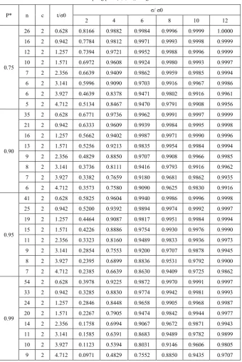
(10)where λ = n F(t;σ). The minimum values of n satisfying the (10) have also been obtained for the same combination of p*, t/σ0as those used in (8) and are given in Table 2 for α = 2.
The operating characteristic of the sampling plan (n,c,t/σ0) gives the probability of accepting the lot. This probability is given by
( ) (1 )
0
c i n i
L p n pci p
i
−
= −
=
∑
(11) [image:3.595.314.553.252.288.2]where λ = n F(t; σ) is treated as a function of σ- the lot quality parameter. It can be seen that operating characteristic is an increasing function of σ. For given P*, t/σ0, the choice of c and n will be made on the basis of operating characteristics. Values of operating characteristics as a function of σ/σ0 for a few sampling plans are given in Table 3.
The producer’s risk is the probability of rejection of the lot when σ ≥ σ0. For a given value of the producer’s risk, say 0.05, one may be interested in finding what value of σ/σ0 is the smallest positive number for which the following inequality holds:
(1 ) 0.95 0
c i n i
n pci p
i
−
− ≥
=
∑
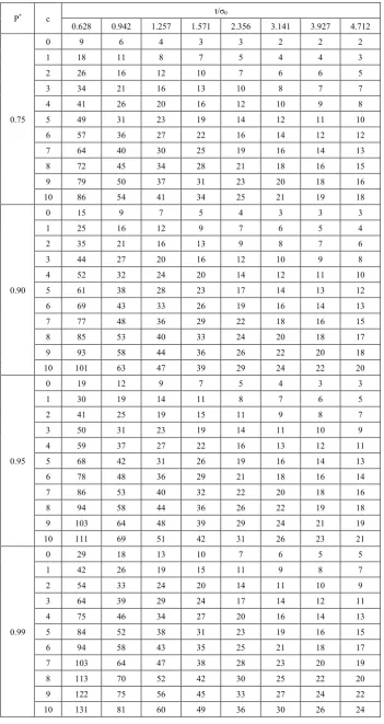
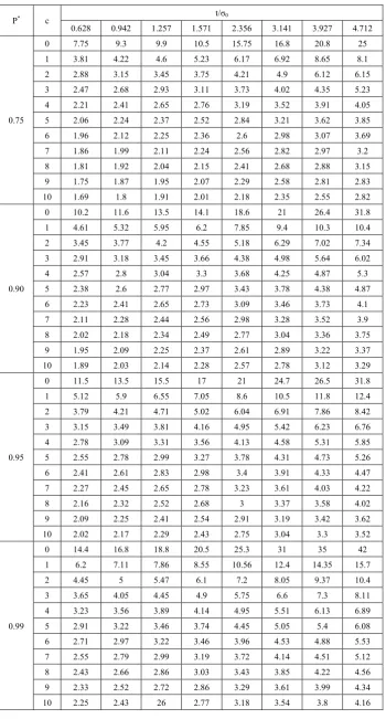
(12)For some sampling plan (n,c,t/σ0) and values of p*, minimum values of σ/σ0 satisfying (12) are given in Table 4.
4. Description of Tables and Examples
Assuming that the life time distribution is a size biased Lomax model, suppose an experimenter is interested in establishing that the true unknown mean is at least 1000hrs with confidence P* = 0.75. It is desired to stop the experiment at t = 628hrs. Then, for an acceptance number c = 2, the required n in Table 1 is 26. If during 628hrs, nomore than 2 failures out of 26 are observed, then the experimenter can assert, with a confidence level of 0.75 that the average life is at least 1000hrs. If the Poisson approximation to binomial probability is used, the value of n from Table 2 is 27.
If the life time distribution is assumed to be a gamma with shape parameter 2 (an IFR model), this value of n from Tables 1 & 2 of Gupta & Groll (1961) is 63 using binomial probabilities and it is 64 using Poisson approximation. Hence it is clear that size biased Lomax model is giving good results when compared to gamma model.
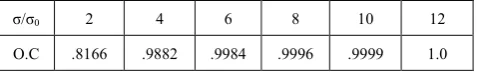
For this sampling plan ( n = 26, c = 2, t/σ0 = 0.628) under the size biased Lomax model, the O.C values from Table 3 are:
σ/σ0 2 4 6 8 10 12
O.C .8166 .9882 .9984 .9996 .9999 1.0
This shows that, if the true mean life is twice the specified mean life (σ/σ0 = 2) the producer’s risk is approximately 0.1834. The producer’s risk is about zero when the true mean life is 12 times than the specified mean life.
Table 1. Minimum sample sizes necessary to assert the mean life to exceed a given value σ0 with P*, at c for α =2( Binomial probabilities).
P* c t/σ0
0.628 0.942 1.257 1.571 2.356 3.141 3.927 4.712
0.75
0 9 6 4 3 3 2 2 2
1 18 11 8 7 5 4 4 3
2 26 16 12 10 7 6 6 5
3 34 21 16 13 10 8 7 7
4 41 26 20 16 12 10 9 8
5 49 31 23 19 14 12 11 10
6 57 36 27 22 16 14 12 12
7 64 40 30 25 19 16 14 13
8 72 45 34 28 21 18 16 15
9 79 50 37 31 23 20 18 16
10 86 54 41 34 25 21 19 18
0.90
0 15 9 7 5 4 3 3 3
1 25 16 12 9 7 6 5 4
2 35 21 16 13 9 8 7 6
3 44 27 20 16 12 10 9 8
4 52 32 24 20 14 12 11 10
5 61 38 28 23 17 14 13 12
6 69 43 33 26 19 16 14 13
7 77 48 36 29 22 18 16 15
8 85 53 40 33 24 20 18 17
9 93 58 44 36 26 22 20 18
10 101 63 47 39 29 24 22 20
0.95
0 19 12 9 7 5 4 3 3
1 30 19 14 11 8 7 6 5
2 41 25 19 15 11 9 8 7
3 50 31 23 19 14 11 10 9
4 59 37 27 22 16 13 12 11
5 68 42 31 26 19 16 14 13
6 78 48 36 29 21 18 16 14
7 86 53 40 32 22 20 18 16
8 94 58 44 36 26 22 19 18
9 103 64 48 39 29 24 21 19
10 111 69 51 42 31 26 23 21
0.99
0 29 18 13 10 7 6 5 5
1 42 26 19 15 11 9 8 7
2 54 33 24 20 14 11 10 9
3 64 39 29 24 17 14 12 11
4 75 46 34 27 20 16 14 13
5 84 52 38 31 23 19 16 15
6 94 58 43 35 25 21 18 17
7 103 64 47 38 28 23 20 19
8 113 70 52 42 30 25 22 20
9 122 75 56 45 33 27 24 22
Table 2. Minimum sample sizes necessary to assert the mean life to exceed a given value σ0 with P*, at c for α =2( Poisson probabilities).
P* c t/σ0
0.628 0.942 1.257 1.571 2.356 3.141 3.927 4.712
0.75
0 10 6 5 4 3 3 3 3
1 19 12 9 8 6 5 5 4
2 27 17 13 11 8 7 7 6
3 35 22 17 14 11 9 9 8
4 43 27 21 17 13 11 10 10
5 50 32 24 20 16 13 12 11
6 58 37 28 33 18 15 14 13
7 66 42 32 26 20 17 16 15
8 73 46 35 29 22 19 18 16
9 81 51 39 32 25 21 19 18
10 88 56 42 35 27 23 21 20
0.90
0 16 10 8 7 5 5 4 4
1 27 17 13 11 8 7 7 6
2 36 23 18 15 11 10 9 8
3 45 29 22 18 14 12 11 10
4 54 34 26 22 17 14 13 12
5 63 40 30 25 19 17 15 14
6 71 45 34 29 22 19 17 16
7 80 51 38 32 24 21 19 18
8 88 56 42 35 27 23 21 20
9 96 61 46 39 29 25 23 21
10 104 66 50 42 32 27 25 23
0.95
0 21 13 10 9 7 6 5 5
1 32 21 16 13 10 9 8 7
2 43 27 21 17 13 11 10 10
3 53 33 25 21 16 14 13 12
4 62 39 30 25 19 16 15 14
5 71 45 34 29 22 19 17 16
6 80 51 39 32 25 21 19 18
7 89 56 43 36 27 23 21 20
8 98 62 47 39 30 26 23 22
9 106 67 51 43 32 28 25 24
10 114 73 55 46 35 30 27 25
0.99
0 31 20 15 13 10 9 8 7
1 45 29 22 18 14 12 11 10
2 57 36 28 23 18 15 14 13
3 68 43 33 27 21 18 16 15
4 78 50 38 32 24 21 19 18
5 89 56 43 36 27 23 21 20
6 98 62 47 40 30 26 23 22
7 108 69 52 43 33 28 26 24
8 117 74 57 47 36 31 28 26
9 127 80 61 51 39 33 30 28
Table 3. O.C values of the sampling plan (n,c,t/σ0) for given P*under SBLM with α = 2.
P* n c t/σ0 σ/ σ0
2 4 6 8 10 12
0.75
26 2 0.628 0.8166 0.9882 0.9984 0.9996 0.9999 1.0000 16 2 0.942 0.7784 0.9812 0.9971 0.9993 0.9998 0.9999 12 2 1.257 0.7394 0.9721 0.9952 0.9988 0.9996 0.9999 10 2 1.571 0.6972 0.9608 0.9924 0.9980 0.9993 0.9997 7 2 2.356 0.6639 0.9409 0.9862 0.9959 0.9985 0.9994 6 2 3.141 0.5996 0.9090 0.9703 0.9916 0.9967 0.9986 6 2 3.927 0.4639 0.8378 0.9471 0.9802 0.9916 0.9961 5 2 4.712 0.5134 0.8467 0.9470 0.9791 0.9908 0.9956
0.90
35 2 0.628 0.6771 0.9736 0.9962 0.9991 0.9997 0.9999 21 2 0.942 0.6333 0.9609 0.9939 0.9984 0.9995 0.9998 16 2 1.257 0.5662 0.9402 0.9987 0.9971 0.9990 0.9996 13 2 1.571 0.5256 0.9213 0.9835 0.9954 0.9984 0.9994 9 2 2.356 0.4829 0.8850 0.9707 0.9908 0.9966 0.9985 8 2 3.141 0.3736 0.8111 0.9416 0.9793 0.9916 0.9962 7 2 3.927 0.3382 0.7659 0.9180 0.9681 0.9862 0.9935 6 2 4.712 0.3573 0.7580 0.9090 0.9625 0.9830 0.9916
0.95
41 2 0.628 0.5825 0.9604 0.9940 0.9986 0.9996 0.9998 25 2 0.942 0.5200 0.9392 0.9894 0.9974 0.9992 0.9997 19 2 1.257 0.4464 0.9087 0.9817 0.9951 0.9984 0.9994 15 2 1.571 0.4226 0.8886 0.9754 0.9930 0.9976 0.9990 11 2 2.356 0.3323 0.8160 0.9489 0.9833 0.9936 0.9973 9 2 3.141 0.2854 0.7553 0.9200 0.9707 0.9878 0.9945 8 2 3.927 0.2395 0.6899 0.8836 0.9531 0.9792 0.9900 7 2 4.712 0.2385 0.6639 0.8630 0.9409 0.9725 0.9862
0.99
Table 4. Minimum ratio of σ/σ0for the acceptability of a lot with 0.05 for α = 2
P* c t/σ0
0.628 0.942 1.257 1.571 2.356 3.141 3.927 4.712
0.75
0 7.75 9.3 9.9 10.5 15.75 16.8 20.8 25
1 3.81 4.22 4.6 5.23 6.17 6.92 8.65 8.1
2 2.88 3.15 3.45 3.75 4.21 4.9 6.12 6.15
3 2.47 2.68 2.93 3.11 3.73 4.02 4.35 5.23
4 2.21 2.41 2.65 2.76 3.19 3.52 3.91 4.05
5 2.06 2.24 2.37 2.52 2.84 3.21 3.62 3.85
6 1.96 2.12 2.25 2.36 2.6 2.98 3.07 3.69
7 1.86 1.99 2.11 2.24 2.56 2.82 2.97 3.2
8 1.81 1.92 2.04 2.15 2.41 2.68 2.88 3.15
9 1.75 1.87 1.95 2.07 2.29 2.58 2.81 2.83
10 1.69 1.8 1.91 2.01 2.18 2.35 2.55 2.82
0.90
0 10.2 11.6 13.5 14.1 18.6 21 26.4 31.8
1 4.61 5.32 5.95 6.2 7.85 9.4 10.3 10.4
2 3.45 3.77 4.2 4.55 5.18 6.29 7.02 7.34
3 2.91 3.18 3.45 3.66 4.38 4.98 5.64 6.02
4 2.57 2.8 3.04 3.3 3.68 4.25 4.87 5.3
5 2.38 2.6 2.77 2.97 3.43 3.78 4.38 4.87
6 2.23 2.41 2.65 2.73 3.09 3.46 3.73 4.1
7 2.11 2.28 2.44 2.56 2.98 3.28 3.52 3.9
8 2.02 2.18 2.34 2.49 2.77 3.04 3.36 3.75
9 1.95 2.09 2.25 2.37 2.61 2.89 3.22 3.37
10 1.89 2.03 2.14 2.28 2.57 2.78 3.12 3.29
0.95
0 11.5 13.5 15.5 17 21 24.7 26.5 31.8
1 5.12 5.9 6.55 7.05 8.6 10.5 11.8 12.4
2 3.79 4.21 4.71 5.02 6.04 6.91 7.86 8.42
3 3.15 3.49 3.81 4.16 4.95 5.42 6.23 6.76
4 2.78 3.09 3.31 3.56 4.13 4.58 5.31 5.85
5 2.55 2.78 2.99 3.27 3.78 4.31 4.73 5.26
6 2.41 2.61 2.83 2.98 3.4 3.91 4.33 4.47
7 2.27 2.45 2.65 2.78 3.23 3.61 4.03 4.22
8 2.16 2.32 2.52 2.68 3 3.37 3.58 4.02
9 2.09 2.25 2.41 2.54 2.91 3.19 3.42 3.62
10 2.02 2.17 2.29 2.43 2.75 3.04 3.3 3.52
0.99
0 14.4 16.8 18.8 20.5 25.3 31 35 42
1 6.2 7.11 7.86 8.55 10.56 12.4 14.35 15.7
2 4.45 5 5.47 6.1 7.2 8.05 9.37 10.4
3 3.65 4.05 4.45 4.9 5.75 6.6 7.3 8.11
4 3.23 3.56 3.89 4.14 4.95 5.51 6.13 6.89
5 2.91 3.22 3.46 3.74 4.45 5.05 5.4 6.08
6 2.71 2.97 3.22 3.46 3.96 4.53 4.88 5.53
7 2.55 2.79 2.99 3.19 3.72 4.14 4.51 5.12
8 2.43 2.66 2.86 3.03 3.43 3.85 4.22 4.56
9 2.33 2.52 2.72 2.86 3.29 3.61 3.99 4.34
[image:7.595.131.482.85.737.2]5. Conclusion
Size biased Lomax distribution, a new probability model is taken as a life time random variable. General introduction to the pdf with necessary characteristics are discussed and a few references are mentioned. The proposed sample plan is discussed with a known shape parameter. We observed the minimum sample size necessary to assure the specified mean life time for various acceptance numbers, confidence levels and values of the ratio of the fixed experimental time to the specified mean life time. The Operating characteristic values are evaluated and are tabulated. The experimental results are compared with the existing sampling plan in which the life time random variable assumes Gamma model. Our proposed sampling plan with SBLM shows good results than the existing sampling plan.
REFERENCES
[1] A.Aa Abdel-Ghaly, A.F. Attia & H.M. Aly. Estimation of the parameters of Pareto distribution and reliability function using accelerated life testing with censoring, Commun. Statist.-Simula., 27(2), 469-484, (1998).
[2] D.R. Cox. Renewal Theory, Barnes & Noble, New York, (1962).
[3] S.S. Gupta & P.A Groll. Gamma distribution in acceptance sampling based on life tests, J. Amer. Statist. Assoc., 56, 942-970, (1961).
[4] R.C. Gupta & H.O. Akman. On the reliability studies of a weighted inverse Gaussian model, Journal of Statistical Planning and Inference, vol 48, 69-83, (1995).
[5] R.R.L. Kantam& K. Rosaiah. Half logistic distribution in acceptance sampling based on life tests. IAPQR Transactions, vol. 23, no. 2, (1998).
[6] R.R.L. Kantam, K. Rosaiah & G. Srinivas Rao. Acceptance sampling based on life tests: log-logistic model, Journal of
Applied Statistics (U.K), vol 28, no. 1, 121-128, (2001).
[7] G. Kulldroff & K. Vannman. Estimation of the location and
scale parameters of a Pareto distribution by linear functions of order statistics, Journal of American Statistical Association (JASA), 68(341), 218-227, (1973).
[8] G.P. Patil. Weighted distributions, Encyclopedia of Environ metrics, John Wiley & Sons, Ltd, Chichester (ISBN 0471 899976) vol 4, 2369-2377, (2002).
[9] C.R. Rao. Weighted distributions arising out of methods of ascertainment, in A Celebration of Statistics, A.C. Atkinson & S.E. Fienberg, eds, Springer-Verlag, New York, Chapter 24, 543-569, (1965).
[10] K. Rosaiah, R.R.L. Kantam & R.Subba Rao. Pareto
distribution in acceptance sampling based on truncated life tests, IAPQR Transcations, 34(1), (2009).
[11] G. Srinivas Rao, M.E. Ghitany & R.R.L. Kantam. Acceptance
sampling plans for Marshall-Olkin extended Lomax distribution, International Journal of Applied Mathematics, vol 21(2), 315-325, (2008).
[12] M. Sobel & J.A. Tisschendrof. Acceptance sampling with new life test objectives. Proceedings of fifth national symposium on Reliability and Quality Control, Philadelpina, Pennsylvania, 108-118, (1959).
[13] K. Vannman. Estimators based on order statistics from a