Evaluation of Model for Air Pollution in the Vicinity of Roadside Solid Barriers

(1)

Evaluation of Model for Air Pollution in the Vicinity

of Roadside Solid Barriers

Desmond Adair

1,*

_{, Martin Jaeger}

2

1_{School of Engineering, Nazarbayev University, Republic of Kazakhstan} 2_{School of Engineering & ICT, University of Tasmania, Australia}

Abstract

Roadside noise barriers and solid fences are common features along major highways in urban regions of Kazakhstan and are anticipated to have important effects on near-road air pollution through altering the dispersion of traffic emissions and resulting downstream concentrations. A 3-dimensional computational fluid dynamics (CFD) road model has been developed to simulate roadside barrier effects on near-road air quality and evaluate the influence of key variables, such as barrier height and wind direction. The CFD model is tested against experimental data and other existing models found in the literature, with several turbulence models tested to give optimal results, i.e., the standard 𝑘𝑘 − 𝜀𝜀 model and the realizable 𝑘𝑘 − 𝜀𝜀 model with different Schmidt numbers. The dispersion of a mixture of nitrogen oxides (denoted as NOx—a mix of NO

and NO2) was computed and the barriers were assumed to

be straight and infinitely long. Dispersion of NOx was

modeled for situations with no barriers along the highway, barriers on both sides, and for a single barrier on the downwind side of the highway. The modelling results are presented and discussed in relation to previous studies and the implications of the results are considered for pollution barriers along highways.

Keywords

CFD Modelling, Roadside Barriers, Near-road Air Pollution

1. Introduction

In a recent study [1] it was concluded that in general, air pollution in Kazakhstan constitutes a significant contribution to the burden of diseases. In relative terms, the impact of air pollution on premature mortality in Kazakhstan is notably higher than in say Russia or the Ukraine. To add to this, public health concerns related to near-road air quality have become a pressing issue, due to the increasing number of epidemiological studies suggesting that populations spending significant amounts of time near heavily trafficked roads are at greater risk of

adverse health effects [2,3]. Emission control techniques and programs are used to directly reduce emitted air pollutants and are an essential part of air quality management, but other strategies such as the planting of trees and bushes and the erection of road-side structures such as noise barriers are used as near-term mitigation strategies. Many roadside solid fences are also erected to hide unsightly building sites, etc. within urban areas in Kazakhstan. These methods, if successful, can provide measures to reduce impacts from sources that are difficult to mitigate [4].

Cars are responsible for high concentrations of both gaseous air pollution and particulates. Nitrogen oxides (NO and NO2) are the most important of the many air pollution

agents that are emitted into the atmosphere. Although the concentration of air pollutants is usually measured, there are a limited number of monitoring stations within a city. Therefore, the spatial distribution of these agents is often modeled rather than measured, particularly for city management and municipal authorities. Many cities use software such as the ADMS-Urban [5] or Gaussian-plume [6] software. Such systems (and others used in Europe and the USA) are used to model concentrations over whole or large parts of cities. In contrast, this study will focus on issues at a local level in close proximity to busy roads and streets in settled areas on the outskirts of large cities. These areas are typically densely populated, with large groups of houses protected from traffic noise by barriers and have solid fences erected for privacy or aesthetic uses.

(2)

concentrations [11-14]. A study in California determined lower pollution levels in the lee of a barrier, relative to a clearing, but that concentrations rose to levels above the clearing further downwind [14] while a field experiment studying the dispersion of a sulphur hexiflouride (SF6) line source upwind of a 6 m high straw bale barrier, constructed to simulate a solid noise barrier, found concentration reductions downwind of the barrier relative to concentrations from the same source in a clearing, for a range of meteorological stability categories [13]. Wind tunnel experiments also show that for crosswind conditions, a roadside barrier leads to a vertical lofting of the roadway emissions and decrease of ground-level concentrations in the wake of a barrier, relative to a no-barrier case [12]. However, despite all these many works, there is still little information of how solid barriers affect pollutant transport, especially under a variety of barrier height and configurations [15]. Also the extent to which double barriers can reduce air pollution near roads, under varying noise-barrier heights remains uncertain [3].

The simulation of the dispersion of air pollution in complex situations, such as in the vicinity of roadside barriers, is difficult, but it has been suggested that progress can be made by building and running models using computational fluid dynamics (CFD) [16]. Therefore, in this work, in order to further understand the conditions that favor or disfavor air quality improvement by roadside barriers, a computational fluid dynamics (CFD) roadside barrier model was developed and tested against experimental results and other recent studies found in the literature.

2. CFD Model

A CFD model has been developed to simulate wind flow and pollutant concentration around both single and double solid roadside barriers. The simulations are based on Reynolds-averaged Navier-Stokes equations (RANS) using closure turbulence models, i.e. the standard 𝑘𝑘 − 𝜀𝜀 model [17] and the realizable 𝑘𝑘 − 𝜀𝜀 model [18], where 𝑘𝑘 is the turbulent kinetic energy and 𝜀𝜀 is the dissipation rate of turbulence kinetic energy.

The continuity and momentum equations for incompressible fluid used are,

𝜕𝜕𝑢𝑢𝑖𝑖

𝜕𝜕𝑥𝑥𝑗𝑗= 0 (1)

𝜕𝜕𝜕𝜕 +𝑢𝑢𝑗𝑗 𝜕𝜕𝑢𝑢𝑖𝑖

𝜕𝜕𝑥𝑥𝑗𝑗=−

1 𝜌𝜌

𝜕𝜕𝜕𝜕 𝜕𝜕𝑥𝑥𝑖𝑖+𝜈𝜈

𝜕𝜕2𝑢𝑢𝑖𝑖

𝜕𝜕𝑥𝑥𝑗𝑗𝜕𝜕𝑥𝑥𝑗𝑗−

𝜕𝜕 𝜕𝜕𝑥𝑥𝑗𝑗�𝑢𝑢𝚤𝚤

′_𝑢𝑢 𝚥𝚥′

��+𝑔𝑔 (2) where, 𝑢𝑢𝑖𝑖 is the jth component of velocity, 𝑡𝑡 is the time,

𝑥𝑥𝑗𝑗 is the jth coordinate, 𝜌𝜌 is the air density, 𝜐𝜐 is the

kinematic viscosity, and 𝑔𝑔 is the gravitational body force. The equation,

−𝑢𝑢𝚤𝚤′𝑢𝑢𝚥𝚥′

��₌_𝜈𝜈_𝜕𝜕_�𝜕𝜕𝑢𝑢𝑖𝑖

𝜕𝜕𝑥𝑥𝑗𝑗+

𝜕𝜕𝑢𝑢𝑗𝑗

𝜕𝜕𝑥𝑥𝑖𝑖� −

2

3𝑘𝑘𝛿𝛿𝑖𝑖𝑗𝑗 (3)

is the Reynolds stress equation, where 𝜈𝜈𝜕𝜕=𝐶𝐶𝜇𝜇𝑘𝑘2⁄𝜀𝜀 is the

turbulent viscosity.

Enlarged-viscosity models became popular in the late 1970’s due to development of the first computers, and rudiments of CFD programs, which allowed the Kolmogorov-type differential equations to be solved. The assumption, on which the standard 𝑘𝑘 − 𝜀𝜀 model is based, implies that once turbulent energy is generated at the low wave number end of the spectrum, it is dissipated at the high wave number end. In turbulent air flow modelling this is generally the case, because of a vast size disparity between those eddies in which turbulence production takes place, and the eddies in which turbulence dissipation occurs [19]. The standard 𝑘𝑘 − 𝜀𝜀 model, examined in this study, employs the eddy viscosity concept and calculates the eddy viscosity using 𝜈𝜈𝜕𝜕=𝐶𝐶𝜇𝜇𝑘𝑘2⁄𝜀𝜀. Here the turbulence energy k

[image:2.595.308.556.391.610.2]

characterizes the intensity of the turbulent fluctuations and the dissipation rate 𝜀𝜀 the length scale of the energy-containing eddies through the relation. The distribution of k and 𝜀𝜀 is determined from the solution of semi-empirical transport equations as in the standard 𝑘𝑘 − 𝜀𝜀 model [20], which is summarized in Table 1.

Table 1. Summarized standard 𝑘𝑘 − 𝜀𝜀 turbulence model

Equation Φ ΓΦ 𝑆𝑆Φ

T. Kinetic Energy 𝑘𝑘 𝜈𝜈𝜕𝜕/𝜎𝜎𝑘𝑘 𝜌𝜌(𝐺𝐺 − 𝜀𝜀) Dissipation Rate 𝜀𝜀 𝜈𝜈𝜕𝜕/𝜎𝜎𝜀𝜀 𝜌𝜌(𝜀𝜀 𝑘𝑘⁄ ) (𝐶𝐶𝜀𝜀1𝐺𝐺 − 𝐶𝐶𝜀𝜀2𝜀𝜀

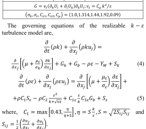
𝐺𝐺=𝜈𝜈𝜕𝜕(𝜕𝜕𝑘𝑘𝑈𝑈𝑖𝑖+𝜕𝜕𝑖𝑖𝑈𝑈𝑘𝑘)𝜕𝜕𝑘𝑘𝑈𝑈𝑖𝑖;𝜈𝜈𝜕𝜕=𝐶𝐶𝜇𝜇𝑘𝑘2⁄𝜀𝜀

�𝜎𝜎𝑘𝑘,𝜎𝜎𝜀𝜀,𝐶𝐶𝜀𝜀1,𝐶𝐶𝜀𝜀2,𝐶𝐶𝜇𝜇�= (1.0,1.314,1.44,1.92,0.09)

The governing equations of the realizable 𝑘𝑘 − 𝜀𝜀 turbulence model are,

𝜕𝜕

𝜕𝜕𝑡𝑡(𝜌𝜌𝑘𝑘) + 𝜕𝜕

𝜕𝜕𝑥𝑥𝑗𝑗�𝜌𝜌𝑘𝑘𝑢𝑢𝑗𝑗�= 𝜕𝜕

𝜕𝜕𝑥𝑥𝑗𝑗��𝜇𝜇+

𝜇𝜇𝑡𝑡

𝜎𝜎𝑘𝑘�

𝜕𝜕𝑘𝑘

𝜕𝜕𝑥𝑥𝑗𝑗�+𝐺𝐺𝑘𝑘+𝐺𝐺𝑏𝑏− 𝜌𝜌𝜀𝜀 − 𝑌𝑌𝑀𝑀+𝑆𝑆𝑘𝑘 (4)

𝜕𝜕 𝜕𝜕𝑡𝑡(𝜌𝜌𝜀𝜀) +

𝜕𝜕

𝜕𝜕𝑥𝑥𝑗𝑗�𝜌𝜌𝜀𝜀𝑢𝑢𝑗𝑗�=

𝜕𝜕 𝜕𝜕𝑥𝑥𝑗𝑗��𝜇𝜇+

𝜇𝜇𝜕𝜕

𝜎𝜎𝜀𝜀�

𝜕𝜕𝜀𝜀 𝜕𝜕𝑥𝑥𝑗𝑗�+

+𝜌𝜌𝐶𝐶1𝑆𝑆𝜀𝜀− 𝜌𝜌𝐶𝐶2 𝜀𝜀

2

𝑘𝑘+√𝜈𝜈𝜀𝜀+𝐶𝐶1𝜀𝜀 𝜀𝜀

𝑘𝑘𝐶𝐶3𝜀𝜀𝐺𝐺𝑏𝑏+𝑆𝑆𝜀𝜀 (5)

where, 𝐶𝐶1= max�0.43,_𝜂𝜂+5𝜂𝜂 �,𝜂𝜂=𝑆𝑆𝑘𝑘_𝜀𝜀,𝑆𝑆=�2𝑆𝑆𝑖𝑖𝑗𝑗𝑆𝑆𝑖𝑖𝑗𝑗 and

𝑆𝑆𝑖𝑖𝑗𝑗 =1₂�𝜕𝜕𝑢𝑢_{𝜕𝜕𝑥𝑥}𝑗𝑗

𝑖𝑖+

𝜕𝜕𝑥𝑥𝑗𝑗�.

Here 𝐺𝐺𝑘𝑘 represents the generation of turbulence energy

due to the mean velocity gradients, 𝐺𝐺𝑏𝑏 is the generation of

turbulence kinetic energy due to buoyancy, and 𝑌𝑌𝑀𝑀represents the contribution of the fluctuating dilatation in

compressible turbulence, to the overall dissipation rate. The model constants are 𝜎𝜎𝑘𝑘(=1.0), 𝜎𝜎𝜀𝜀 (=1.2), 𝐶𝐶1𝜀𝜀(=1.44),

𝐶𝐶2(=1.9). The degree to which 𝜀𝜀 is affected by the

buoyancy is determined by the constant 𝐶𝐶3= tanh|𝑣𝑣 𝑢𝑢⁄ |

(3)

species transport equation, in conjunction with the turbulence model equations. The mass diffusion process was based on the following equations [16, 21],

𝐽𝐽𝑖𝑖=− �𝜌𝜌𝐷𝐷𝑖𝑖+_{𝑆𝑆𝑆𝑆}𝜇𝜇𝑡𝑡_𝑡𝑡� ∇𝑦𝑦𝑖𝑖 (6)

where, 𝐽𝐽𝑖𝑖 is the diffusion flux of the mixture, 𝜌𝜌 is the

density of the mixture, 𝐷𝐷𝑖𝑖 is the mass diffusion coefficient

of the pollutant in the mixture, 𝑦𝑦𝑖𝑖 is the mass fraction of

the pollutant, and 𝜇𝜇𝜕𝜕 is the turbulent viscosity. The

turbulent Schmidt (𝑆𝑆𝑆𝑆𝜕𝜕) was set at 0.7 - 1.3 [16, 22].

3. Geometry and Boundary Conditions

[image:3.595.311.553.156.205.2]

A 3-dimensional CFD simulation of a generic highway was designed. The atmospheric boundary layer for these studies had neutral boundary condition, The CFD modeled scenario consists of a six-lane divided highway which serves as a source of turbulence and emissions of an inert gaseous tracer with the same density as air. Figure 1 shows a schematic of a section of the computational mesh in the vicinity of double roadside barriers. The mesh was reasonably fine here but was gradually coarsened away from solid surfaces.

Figure 1. Computational mesh in vicinity of double roadside barriers

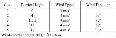
Table 2. Single barrier studies

Case Barrier Height Wind Speed Wind Direction 1

2 3 4 5

0 H*

1.5H H H

4 m/sa

- 90° 90° 60° 30°

a_{Wind speed at height 20H,}*_{H = 6 m}

The model for single barriers is oriented with the solid barrier on the downwind side of the roadway, with the model domain extending 800 m downwind of the roadway. In near-road field studies, air pollution impact from major roadways is commonly detected at distances of several hundred meters, although under unique meteorological conditions the spatial extent of near-road air pollution can be up to several kilometers [23]. This model domain is designed to focus on impacts within several hundred meters of a road. For scenarios with perpendicular winds, the model domain is 2000 m along the road axis, 900 m perpendicular to the road, and 200 m in height. The model has a graduated Cartesian mesh, ranging from 0.25 m in close proximity to the barrier and increasing with distance from the road/barrier to 10 m maximum. Multiple model

scenarios as given in Table 2, changing barrier height and wind direction, and observing the impact on traffic-related emissions dispersion and resulting near-road air quality were then carried out.

[image:3.595.61.295.369.455.2]

For double barrier studies:

Table 3. Double barrier studies

Case Barrier Height Wind Speed Wind Direction 1

2 1.5H H 12 m/s

b

12 m/sb 90° _90°

b_{Wind speed at height 83.3H}

For the single barrier studies, the modelled scenario matches an existing wind tunnel model [12], in terms of road configuration and atmospheric boundary layer properties. A solid 6 m (1H) high and variations (see Table 2) and 0.5 m thick wall is located along one side of the highway. The barrier height chosen was chosen in part to validate the model against experimental results. There can be found a great variation in barrier heights, depending on, amongst other things, terrain and local wind conditions. It is known, that from a noise reduction point of view that each additional metre in height of barrier above the source/receiver line of sight gives an additional 1.5 dB of noise level reduction [24]. Typical noise barrier ranges from 4 m to 7 m [25]. For the wind tunnel matching simulation, the wall was continuous throughout the domain and located 3.9 m from the nearest lane of traffic. In the CFD simulations that followed, the wall dimensions more closely matched a site where field data have been collected [8] where a 6 m high, 0.5 m thick wall that is located at 5 m from the nearest lane of traffic, and having a discrete length. In the model, the wall spans 750 m of the roadway, with no obstructions to flow for a stretch of the roadway before and after. This design allows changes in the pollutant dispersion due to the barrier to be directly assessed relative to the clearing and also allows the effect of the barrier edges to be observed. A similar computational domain size was used for the double barrier cases, although a different inlet wind profile was chosen as will be detailed below.

The upstream profile was chosen to represent pedestrian-level wind conditions. Much has been written concerning which profile to use. For example [26] proposed inflow boundary conditions of mean wind speed and turbulence quantities for the standard 𝑘𝑘 − 𝜀𝜀 model which satisfied the transport equations for 𝑘𝑘 and 𝜀𝜀. This is a commonly found boundary condition for wind engineering. Another upstream condition was proposed [27] where again the solution of the turbulence energy equation associated with the standard 𝑘𝑘 − 𝜀𝜀 was solved yielding a new set of inflow turbulence boundary conditions.

The inlet boundary condition for 𝑢𝑢 in the neutral boundary condition is,

𝑢𝑢(𝑧𝑧) =𝑢𝑢_𝑘𝑘∗ln�1 +_𝑧𝑧𝑧𝑧

0� (8)

where, 𝑢𝑢∗_{is the friction velocity,}_𝑘𝑘_{is the von Karman}

constant, 𝑧𝑧0 is the roughness length and 𝑧𝑧 is the height

[image:3.595.58.297.496.575.2]

(4)

between turbulence dissipation and production is assumed, the profile for 𝑘𝑘 and 𝜀𝜀 has the form,

(𝑧𝑧) =�𝐴𝐴ln(𝑧𝑧+𝑧𝑧0+𝐵𝐵 (8)

[image:4.595.59.299.197.454.2]

where, 𝐴𝐴 and 𝐵𝐵 are constants that can be determined by fitting the equations to the measured profiles of 𝑘𝑘. Using wind tunnel results [12], for the profile under consideration, 𝐴𝐴=−0.075 and 𝐵𝐵= 0.478 were selected in this study.

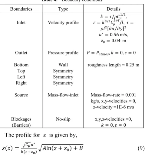
Table 4. Boundary conditions

Boundaries Type Details

Inlet

Outlet

Bottom Top Left Right

Source

Blockages (Barriers)

Velocity profile

Pressure profile

Wall Symmetry Symmetry Symmetry

Mass-flow-inlet

No-slip

𝑘𝑘=𝜏𝜏/𝜌𝜌𝐶𝐶𝜇𝜇1/2,

𝜀𝜀=𝑘𝑘3/2_𝐶𝐶 𝜇𝜇3/4/𝑙𝑙, 𝜏𝜏=

𝜌𝜌𝑙𝑙2_[_{𝜕𝜕𝑢𝑢 𝜕𝜕𝑦𝑦}_⁄ _]2

𝑢𝑢∗_{= 0.56}_m/s,

𝑧𝑧0= 0.04 m

𝑃𝑃=𝑃𝑃𝑎𝑎𝜕𝜕𝑎𝑎𝑎𝑎𝑎𝑎,𝑘𝑘= 0,𝜀𝜀= 0

roughness length = 0.25 m

Mass-flow-rate = 0.001 kg/s, x,y-velocities = 0,

z-velocity =1E-6 m/s

x,y,z-velocities =0,

𝑘𝑘= 0,𝜀𝜀= 0 The profile for 𝜀𝜀 is given by,

𝜀𝜀(𝑧𝑧) = �𝐶𝐶𝜇𝜇𝑢𝑢∗

[image:4.595.319.541.346.471.2]

𝑘𝑘(𝑧𝑧+𝑧𝑧0)�𝐴𝐴ln(𝑧𝑧+𝑧𝑧0) +𝐵𝐵 (9)

Table 4 lists the boundary conditions used in this study [29], where the roughness length and friction velocity are those found in [30] and [31] respectively. The composition of NOx at emission corresponded to 70% NO2 and 30% NO,

and this remained constant over the time and distance modelled. The emission rate of NOx used was set at 0.222

g/s/km per lane of traffic [32].

4. Results and Discussion

A major part of developing a suitable CFD model suitable to calculate the dispersion of pollutants in the vicinity of solid barriers was the selection of a suitable closure model. As already stated, the 𝑘𝑘 − 𝜀𝜀 turbulence model with standard wall functions and the realizable 𝑘𝑘 − 𝜀𝜀 turbulence model with various Schmidt numbers (the ratio of the turbulent transfer of momentum in the form of turbulent viscosity to the turbulent transfer of mass in the form of turbulent diffusivity) were used. The role of this important parameter has not been exported extensively within urban areas but values from 0.18 to 1.34 have been suggested in the literature [33]. In this work for wind tunnel comparison values of 𝑆𝑆𝑆𝑆𝜕𝜕 of 0.7, 1.0 and 1.3 were selected.

Here, the concentrations of NOx have been normalized to

give the non-dimensional concentration 𝜒𝜒=𝐶𝐶𝑈𝑈𝑟𝑟𝐿𝐿𝑥𝑥𝐿𝐿𝑦𝑦⁄𝑄𝑄

[12], where 𝐶𝐶 is the concentration (a fraction by mass) with background concentration subtracted, 𝑈𝑈𝑟𝑟 is the

reference wind speed measured at a full-scale equivalent height of 500 m), 𝑄𝑄 is the mass flow (0.01 kg/s of CO), 𝐿𝐿𝑥𝑥 is along the wind direction of the road (30 m), and 𝐿𝐿𝑦𝑦

is the lateral length of the source segment. As can be seen on Figure 2 the standard and realizable 𝑘𝑘 − 𝜀𝜀 turbulence models produce fairly reasonable concentration profiles in the 𝑧𝑧 direction for the 1H barrier case and with X/H = 7. However the standard 𝑘𝑘 − 𝜀𝜀 and the realizable 𝑘𝑘 − 𝜀𝜀 with 𝑆𝑆𝑆𝑆𝜕𝜕 of 0.7 turbulence models clearly under-predict the

ground-level concentration while the realizable 𝑘𝑘 − 𝜀𝜀 with 𝑆𝑆𝑆𝑆𝜕𝜕 of 1.3 over-predicts the ground-level concentration.

When 𝑆𝑆𝑆𝑆𝜕𝜕is set to 1, the results are fairly satisfactory.

Similar results were found when no barrier was present and when X/H = 20. It was decided therefore, for the rest of the study to use the realizable 𝑘𝑘 − 𝜀𝜀 with 𝑆𝑆𝑆𝑆𝜕𝜕 of 1.0. Figure 3

shows a comparison between the calculated and experimental results of surface concentrations at 𝑧𝑧= 1 m height with no barrier present and with 𝑆𝑆𝑆𝑆𝜕𝜕= 1.0. As can

[image:4.595.321.542.511.645.2]

be seen a reasonably good comparison was found.

Figure 2. Comparison of wind tunnel and CFD concentration profiles with a barrier of 1H at X/H =7

Figure 3. Comparison of experimental and the current simulation model results with no barrier present and at 𝑧𝑧= 1 m

(5)

[image:5.595.58.295.179.265.2]

of the barrier with increasing height (Figure 4). Also noted on Figure 4 is a recirculating zone downwind of the barrier and this mixing zone extends vertically upwards and slightly exceeds the barrier height. The length of the mixing zone is approximately 10-12 times the barrier height. The gradient of the velocity in the vicinity of the barrier top edge and downwind of the barrier generates turbulent kinetic energy. This increases with barrier height,

Figure 4. Velocity vectors in the presence of a 1H barrier

After completing the selection of the realizable turbulence model with 𝑆𝑆𝑆𝑆𝜕𝜕= 1.0 a series of flows were

calculated for concentration values as detailed in Tables 2 and 3. A simple graduated Cartesian mesh was used throughout these investigations, moving from course to finer meshes for each calculation until the results showed no ‘grid dependency’. Typical values for the maximum mesh size for flow with one barrier was around 0.5 million with a resultant CPU time of approximately 8-12 hours.

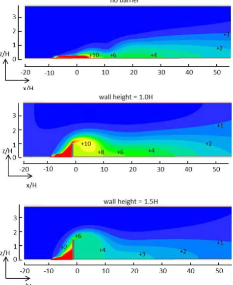
The vertical lofting of on-road emissions leads to reduced concentrations of NOx at the ground level, relative to the

[image:5.595.313.551.184.475.2]

no-barrier case as shown by the concentration contours of Figure 5. For example, the 𝜒𝜒= 4 contours extends further downstream by some 15% for the case with no barrier compared to the 1H barrier calculation.

When the barrier height is increased it would appear that the concentration of NOx reduces behind the barrier as

shown for the case when the barrier height is set at 1.5H. This is in line with experimental finding [12, 13]. However there have been other studies [11, 14] which suggest that roadside barriers may lead to higher pollutant levels at greater distances from the road, when the vertically lofted traffic emissions plume reattaches. This was not found in this model. It can also be seen from these few studies that the vertical concentration profiles are influenced by different barrier heights. Also maximum concentration behind the barrier is reduced with height. Comparing maximum concentrations of NOx in the near wake of the

barriers 1H and 1.5H, reduction of some 40% was found and it is anticipated that this reduction would grow with barrier height.

The majority of current field and wind tunnel results investigating barrier effects on near road air quality focuses on winds perpendicular to the road. The work here extends that analysis to the effect of oblique wind directions (cases 4 and 5 of Table 2). It is especially interesting to understand the effect of the barrier end-points with changing wind direction. Plan views of model results are shown on Figure 6 for concentration contours of 𝜒𝜒 at 2 m about the ground

[image:5.595.315.551.516.698.2]

for wind directions at 60 and 30 degrees to the solid barrier. It can be seen that there are reasonably high concentrations of pollutant downwind of the barrier due to spill-over of accumulated traffic emissions. This spill-over effect has also been noted [8]. It can be seen for the oblique winds that the region of highest near-road concentrations shifts to the far edge of the barrier, while a reduced concentration zone of NOx appears downwind of the other end of the barrier.

Figure 5. Concentration of NOx contours (𝜒𝜒) with orthogonal winds for

the cases, no barrier, a barrier height of 1H and of 1.5H

Figure 6. Plan view of concentration of NOx contours (𝜒𝜒) at 2 m above

ground surface with a barrier height of 1H for wind directions of 60° and 30°.

(6)

oblique wind affects the on-road concentrations, with less accumulated concentrations being noted with greater angles to the barrier.

[image:6.595.316.547.228.371.2]

Figure 7 shows a typical result for concentration contours (𝜒𝜒) for a double barrier case. The concentration contours for different barrier heights reveal that the double solid barriers height changes the vertical location of maximum concentration, downwind of the road. The presence of a double barrier was found to lead to a vertical lofting of emissions with increasing barrier height. Far wake ground level concentrations were found to reduce with the presence of double barriers relative to the no-barrier case whereas in the near-wake significant air pollution impact from the road traffic was predicted up to 100 - 150 m downwind. This is reasonably in line with experimental findings [34, 23].

Figure 7. Typical concentration of NOx contours (𝜒𝜒) for a double barrier

for a barrier height of 1.5H

[image:6.595.60.294.266.358.2]

To show the concentration retention of double road barriers, normalized concentrations between the double solid barriers (horizontal distances are from 0 to 40 m) at 𝑧𝑧= 1 m height are shown on Figure 8.

Figure 8. Normalized average concentrations of NOx between the road

barriers at 𝑧𝑧= 1 m and at the barrier top height (𝑧𝑧= 6 m)

Normalized surface concentrations between the barriers are larger than that of the no barrier case. These increases of normalized concentrations increase with the increase of the solid barrier height. At the top of the barrier however normalized concentration are found to be smaller than those of the surface distribution.

Some results are now given for calculations of NOx

concentrations in terms of µg/m3_{to facilitate discussion}

in terms of regulatory aspects. For example, [35] it is generally accepted that nitrogen dioxide should not exceed

200 µg/m3_{(1 hour mean) more than 18 times per year and}

40 µg/m3_{as the annual mean. It is clear, especially for the}

double barriers that such low figures would be difficult to achieve in the road area. Taking a height of 1.5 m above the ground, time averages of the horizontal NOx concentrations

[image:6.595.66.291.451.600.2]

distributions with and without barriers are shown on Figure 9. It is very clear that the highest concentrations at this height are found in the road area when two barriers are present and to a lesser extent when one barrier is present, with the peak here moved slightly downwind. When no barrier is present the concentration peak is much lower and moved downwind away from the road area.

Figure 9. Time averages of the horizontal NOx concentration profiles (µg/m3₎_{at a height of 1.5 m above the ground}

The distributions are influenced by the recirculation zones behind the barrier and there is some evidence of several maxima over each car lane. Clearly from a regulatory point of view when no barrier exists the concentrations of NOx are relatively low in the road area but

become higher adjacent to the road, possibly causing problems for pedestrians or more importantly residents in that area. Also the value obtained for within the road area is greatly in excess of that proposed by regulatory bodies and during ‘rush hours’ the limit aspired to could be broken daily.

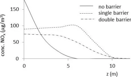
Vertical profiles of NOx concentrations, again given in µg/m3_{are shown on Figure 10 at 10 m from the downwind}

edge of the highway.

Figure 10. Time averages of the vertical NOx concentration profiles

[image:6.595.316.547.588.724.2]

(7)

It can be seen that when barrier(s) are present there is a reduction of in concentration at ground level and an increase in the height at which higher concentrations occur, due to the blocking effect of the barrier and the recirculation behind the barrier. The barriers have the good effect of placing pollution higher in the atmosphere away from pedestrians and residents in their near wakes, with the double barriers more effective than the single barrier.

5. Conclusions

Roadside barriers have many positive uses, including the reduction of noise and aesthetic properties from major traffic corridors in urban regions. This study details the development of a CFD computer model suitable for predicting concentration ‘black-spots’ of pollution due in part to the position, height and length of these barriers. The realizable 𝑘𝑘 − 𝜀𝜀 turbulence model with a Schmidt number of 1.0 was found as the most suitable closure model. Various single and double barrier scenarios were presented with reasonable and plausible results found in comparison to experimental and other simulations found in the literature. It is clear that the presence of barriers has a detrimental effect on the quality of air within the road area but can help with more efficient dispersion downwind of the barriers.

REFERENCES

[1] U. Kenessariyev, A. Golub, M. Brody, A. Dosmukhametov,

M. Amrin, A. Erzhanova, D. Kenessary, Human health cost of air pollution in Kazakhstan, Journal of Environmental Protection, Vol. 4, 869-876, 2013.

[2] HEI, Traffic-related air pollution; a critical review of the

literature on emissions, exposure, and health effects, HEI special report 17, Boston, MA, Health Effects Institute, 2010.

[3] S. J. Jeong, Effect of double noise-barrier on air pollution

dispersion around road, using CFD, Asian Journal of Atmospheric Environment, Vol. 8, No. 2, 81-88, 2014.

[4] H. L. Brantley, G. S. W. Hagler, P. J. Deshmukh, R. W.

Baldauf, Field assessment of the effects of roadside vegetation on near-road black carbon and particulate matter, Science of the Total Environment, Vol. 468-469, 120-129, 2014.

[5] J. Stocker, C. Hood, D. Carruthers, C. McHugh,

ADMS-Urban: Developments in modelling dispersion from the city scale to the local scale, International Journal of Environment and Pollution, Vol. 50, 308-316, 2011.

[6] N. Kh. Arystanbekova, Application of Gaussian plume

models for air pollution simulation at instantaneous emissions, Mathematics and Computers in Simulation, Vol. 67, 451-458, 2004.

[7] Y. F. Zhu, W. C. Hinds, S. Kim, C. Sioutas, Concentration

and size distribution of ultrafine particles near a major highway, Journal of the Air & Waste Management

Association, Vol. 52, 1032-1042, 2002.

[8] R. Baldauf, E. Thoma, V. Isakov, T. Long, J. Weinstein, I.

Gilmour, S. Cho, A. Khlystov, F. Chen, J. Kinsey, M. Hays, R. Seila, R. Snow, R. Shores, D. Olson, B. Gullett, S. Kimbrough, N. Watkins, P. Rowley, J. Bang, D. Costa, Traffic and meteorological impacts on near road air quality: summary of methods and trends from the Raleigh Near Road Study, Journal of the Air & Waste Management Association, Vol. 58, 865-878, 2008.

[9] B. Beckerman, M. Jerrett, J. R. Brook, D. K. Verma, M.A.

Arain, M. M. Finkelstein, Correlation of nitrogen dioxide with other traffic pollutants near a major expressway, Atmospheric Environment, Vol. 42, 275-290, 2008.

[10] G. S. W. Hagler, R. W. , Baldauf, E. D. Thoma, T. R. Long, R. F. Snow, J. S. Kinsey, L. Oudejans, B. K. Gullett, Ultrafine particles near a major roadway in Raleigh, North Carolina: downwind attenuation and correlation with traffic related pollutants, Atmospheric Environment, Vol. 43, 1229-1234, 2009.

[11] G. E. Bowker, R. Baldauf, V. Isakov, A. Khlystov, W.

Petersen, The effects of roadside structures on the transport and dispersion of ultrafine particles from highways, Atmospheric Environment, Vol. 41, 8128-8139, 2007. [12] D. K. Heist, S. G. Perry, L. A. Brixey, A wind tunnel study of

the effect of roadway configurations on the dispersion of traffic-related pollution, Atmospheric Environment, Vol. 43, 5101-5111, 2009.

[13] D. Finn, K. L. Clawson, R. G. Carter, J. D. Rich, R. M.

Eckman, S. G. Perry, V. Isakov, D. K. Heist, Tracer studies to characterize the effects of roadside noise barriers on near-road pollutant dispersion under varying atmospheric stability conditions, Atmospheric Environment, Vol. 44, 204-214, 2010.

[14] Z. Ning, N. Hudda, N. Daher, W. Kam, J. Herner, K. Kozawa,

S. Mara, C. Sioutas. Impact of roadside noise barriers on particle size distributions and pollutants concentrations near freeways, Atmospheric Environment, Vol. 44, 3118-3127, 2010

[15] J. T. Steffens, D. K. Heist, S. G. Perry, K. M. Zhang,

Modeling the effects of a solid barrier on pollutant dispersion under various atmospheric stability conditions, Atmospheric Environment, Vol. 69, 76-85, 2013

[16] A. Riddle, D. Carruthers, A. Sharpe, C. M. J. Stocker,

Comparisons between FLUENT and ADMS for atmospheric dispersion modeling. Atmospheric Environment, Vo. 38, 1029-1038, 2004.

[17] B. E. Launder, D. B. Spalding, The numerical computation of turbulent flows, Computer Methods in Applied Mechanics and Engineering, Vol. 3, No. 2, 269-289, 1974.

[18] T.-H. Shih, W. W. Liou, A. Shabbir, Z. Yang, J. Zhu, A new

𝑘𝑘 − 𝜀𝜀 eddy-viscosity model for high Reynolds number turbulent flows - model development and validation, Computers & Fluids, Vol. 24, No. 3, 227-238, 1995.

[19] B. E. Launder, B. Spalding, Mathematical Models of

Turbulence, Academic Press, London, 1972.

[20] M. A. Leschziner, W. Rodi, Calculation of annular and twin

(8)

352-360, 1981.

[21] W. Y. Ng, C. K. Chau, A modeling investigation of the

impact of street and building configurations on personal air pollutant exposure in isolated deep urban canyons, Science of the Total Environment, Vol. 468-469, 429-448, 2014.

[22] S. D. Sabatino, R. Buccolieri, B. Pulvirenti, R. Britter,

Simulations of pollutant dispersion within idealized urban-type geometries with CFD and integral models, Atmospheric Environment, Vol. 41, 8316-8329, 2007. [23] S. S. Hu, S. Fruin., K. Kozawa, S. Mara, S. E. Paulson, A. M.

Winer, A wide area of air pollutant impact downwind of a freeway during pre-sunrise hours, Atmospheric Environment, Vol. 43, 541-2549, 2009.

[24] US Department of Transportation, Federal Highway

Administration, Noise Barrier Design Handbook, February, 2000.

[25] D. Good, D. Hallden, The design and construction of a noise

barrier along the Vanier highway in Fredericton, Conference of the Transportation Association of Canada, Fredericton, New Brunswick, 2012.

[26] P. J. Richards, R. P. Hoxey, Appropriate boundary conditions for computations for computational wind engineering models

using the 𝑘𝑘 − 𝜀𝜀 model, Journal of Wind Engineering and

Industrial Aerodynamics, Vol. 46-47, 145-153, 1993.

[27] Y. Yang, M. Gu, S. Chen, X. Jin, New inflow boundary

conditions for modelling the neutral equilibrium atmospheric boundary layer in computational wind engineering, Journal of Wind Engineering and Industrial Aerodynamics, Vol. 97, No. 2, 88-95, 2009

[28] C. Gorle, J. Beeck, P. Rambaud, G. V. Tendeloo, CFD

modelling of small particle dispersion: The influence of the turbulence kinetic energy in the atmospheric boundary layer. Atmospheric Environment, Vol. 43, 673-681, 2009.

[29] D. Adair, Numerical calculations of aerial dispersion from

elevated sources, Applied Mathematical Modelling, (1990), Vol. 14, 459-467, 1990.

[30] C. S. B. Grimmond, T. S. King, M. Roth, T. R. Oke,

Aerodynamic roughness of urban areas derived from wind

observations.Boundary-Layer Meteorology, Vol. 89, 1–24,

1998.

[31] J. Hernandez, A. Crespo, Wind turbine wakes in the

atmospheric surface layer, PHOENICS Journal, Vol. 3, No.3, 1990.

[32] European Community, Council directive 1999/30/EC of 22

April 1999 relating to limit values for sulphur dioxide, nitrogen dioxide and oxides of nitrogen, particulate matter and lead in ambient air, Official journal of the EC L 163: 0041–0060, 1999.

[33] T. K. Flesch, J. H. Prueger, J. L. Hatfield, Turbulent Schmidt number from a tracer experiment, Agricultural and Forest Meteorology, Vol. 111, 299-307, 2002.

[34] G. S. W. Hagler, W. Tang, M. J. Freeman, D. K. Heist, S. G.

Perry, A. F. Vette, Model evaluation of roadside barrier impact on near-road air pollution, Atmospheric Environment, Vol. 45, 2522-2530, 2011.

[35] DEFRA (UK), Local Air Quality Management, Part IV of