Impact localisation of a smart composite panel using wave velocity propagation

Impact Localisation of a Smart Composite Panel using Wave Velocity

Propagation

S. Mahzan1,*, W.J. Staszewski2

1_{Faculty of Mechanical and Manufacturing Engineering}

Tun Hussein Onn University of Malaysia (UTHM) Parit Raja, Batu Pahat, 86400 Johor

Malaysia

2_{Department of Mechanical Engineering}

University of Sheffield, Mappin Street, Sheffield S1 3JD United Kingdom

*corresponding author [email protected]

Abstract:

The susceptibility of composite to withstand impact damage challenge the existing maintenance technologies related to damage detection. The problem of impact localisation in composite structures requires a reliable technique for impact damage detection. This paper investigates the reliability of strain data for impact damage localisation. A finite element model has been developed to simulate the impact strain wave propagation which can be used to ease the signal processing data. A series of impacts is experimentally performed on a smart composite panel instrumented with low-profile, embedded piezoceramic transducers. Two wave velocity propagation characteristics are developed using the strain data from both the simulation and experimental works. A Genetic Algorithm, together with the modified triangulation/ multilateration procedure utilises the strain wave velocities propagation for impact positioning. The result shows that the finite element model can assist the experimental work for impact localisation in composite panel with less than 2 percent of total error per area.

.

1. Introduction

The use of composite materials has been widely accepted in many engineering applications. The high strength-to-weight ratio in composites is the main reason why these materials have regularly been chosen. Unfortunately, susceptibility of composite materials to impact damage has led many researchers to study various aspects of composite materials [1-2]. In general, damage detection research can be divided into active and passive methods. Active

techniques based on non-destructive testing (NDT) and structural health monitoring (SHM) techniques. These techniques employ passive or active approaches.

Impact damage detection can be used to estimate impact location and energy. Initial studies of acoustic waves produced by low-velocity impacts have been investigated in [5]. The estimation of impact location and energy/force can be obtained using advanced signal processing techniques. Several of the damage detection methods have been applied to characterise the damage location and classification. These include Artificial Neural Network (ANN), triangulation procedure, Genetic Algorithm (GA) and wavelet approach [6-8]. Some simulation and modelling studies of impact damage detection have also been performed [9-10]. The method utilised a structural model which was used to obtain dynamic responses for simulated impact locations. Therefore in this paper; the aim is to compare the impact location obtained from the simulated strain signal with the experimental works.

2. Methodology

2.1 Finite Element Modelling

This research has employs the commercial finite element (FE) software

package ANSYS 7.0 to develop a simple

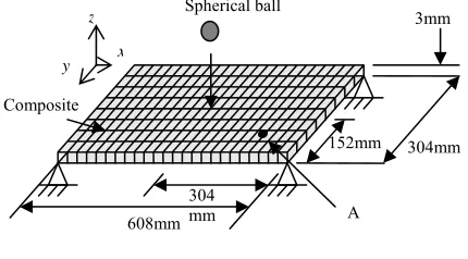
three-dimensional model of a metallic ball impacting a composite plate. In this model the ball is dropped onto the plate, as illustrated in Figure 1. The objective of this investigation is to model the propagation of strain waves in the composite plate resulting from the impact.

The impactor is a spherical steel ball of 15mm diameter whereas the target is a

rectangular composite plate of 608mm ×

304mm × 3mm. The material properties for

the steel ball and the composite plate are given in Table 1. The graphite/epoxy composite plate consists of 16 plies with a

ply sequence of [0/90/45/-45]2s. A SMART

Layer® [11] of transducers was embedded

between the uppermost and subsequent lamina of the plate. However, for simplicity this layer of transducers was not modelled in the current FE work.

z

x y

Spherical ball

3mm

152mm 304mm

A 304

mm 608mm Com

Figure 1: Illustration of FE impact modelling of the composite plate.

Table 1: Material properties of composite lamina and steel ball

Physical

Properties Lamina Steel ball

Young Modulus

[GPa] E2= E3= 8.9 E1 = 160.0, E = 200

Modulus of

Rigidity [GPa] G12= G13 = G23 = 3.45 G = 77.5

Poisson’s ratio V12 = 0.28 V12 = 0.29

Density [kg/m3_]

1545 7972

The SHELL99 element was selected

for the impact modelling work. It consists of 8 nodes with six degrees of freedom per node [12]. The composite plate was uniformly meshed with square shell

elements of 4mm × 4mm, resulted in 23105

elements and 35113 nodes used in the model. Two other element types used in the

impact modelling work were the TARGE170

and CONTA174 elements [12]. These

elements modelled the impact event between the ball and the composite plate. The composite plate was simply supported at each corner. The transient loading was selected in the FE model that determines the

dynamic response of a structure under a time-varying load.

2.2 Genetic Algorithm with modified multilateration procedure

A genetic algorithm (GA) is an optimisation algorithm based on the principles of natural selection and natural genetics, developed in the 1970s by Holland [13]. GAs are designed to mimic natural biological evolution, i.e. inheritance, mutation, reproduction and crossover. GAs offer an alternative way to find optimal solutions close in performance to the global optimum (i.e. maximum or minimum) value.

Figure 2: Illustration of the modified multilateration location procedure [7].

When an impact event occurs, the monitored structure deflects and strain waves propagate outwards in all possible directions; and the task is to estimate the position of this source. A modified multilateration procedure require three

different transducers, labelled as S1, S2 and

S3, to detect these strain waves, as illustrated

in Figure 2. The waves propagate from the unknown impact position towards these transducers. In the currently used impact location procedure, three different

angles,α₁,α₂ andα₃, are randomly assumed

for wave propagation directions. For every

transducer Si and assumed wave propagation

angle αi , the distance di between the

d

transducer and the unknown impact position can be calculated as

where

arrivals and velocities of the propagating

i = vi ti (i=1, 2, 3) (1)

ti and vi are the respective

time-of-strain waves. The ti can be estimated from

the experimental strain data for all relevant transducers. The major difficulty is that the

velocity vi depends on the wave propagation

direction for anisotropic materials. However, the velocity characteristics v_i = f

( )

estimated a priori for monitored composite

structures using experimental analysis and/or FE modelling for all possible angles of wave propagation.

For the assumed wave propagation

directions

{ }

{ }

the analysis of strain data from three

different sducers results in t e

estimated impact positions, i.e. A

d ,

tran hre

The finite element modelling results ated. The focus was the

1, A2 and

A3. These positions can be considered as

vertices of a triangle. GA can then be used to minimise either the area or the total sum of all sides of this triangle. This finally leads to

one estimate for the x and y coordinates of

the unknown impact position.

3. Experimental Works

were experimentally valid

on wave propagation velocities. A

composite plate with the same dimensions and lay-up as the FE model was employed in

this experiment. A SMART® Layer was

embedded between the uppermost and subsequent lamina of the plate. This layer,

manufactured by Acellent Ltd, constituted 12

piezoceramic transducers (6.5mm diameter and 0.25mm thickness) on a Kapton circuited layer. Figure 3 gives the impact and transducer positions. An impact hammer was

used to produce impacts. The LeCroy

Waverunner LT-264 oscilloscope was used to

capture and display all strain data from the impact events with a sampling frequency of 5

A1 A2

A3

S1

S3

S2

α3

α2

α1

Composite structure Piezoceramic sensor

d1

d2

kHz. The experimental setup is shown in Figure 4.

Figure 3: A composite plate embedded with 12 piezoceramic sensors

Figure 4: Experimenta setup for low-velocity

. Results and Discussion

a comparison betwee

l

impacts on the composite plate

4

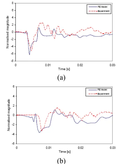
Figure 5 shows

n the normalised simulated and experimental results. A zero-mean type of normalisation was used in this measurement. The calculation of data normalisation is as follow:

i i i i

x x

σ μ

− =

∧

(2)

where is the normalised data, xi is the

i-∧

i x

th component of the original data, μi and σi

are the mean and standard deviation of the original data respectively.

(a)

(b)

Figure 5: Comparison between the FE and

experimental results for: (a) sensor 5 (x=76

mm, y=152 mm), (b) sensor 12 (x=532 mm,

y=252 mm).

Although the experimental strain waves and FE modelling results do not exactly match, the shape of both waves is similar. In fact, the arrival times for the local impact minimum peak differ only by 9.5% and 12% respectively (the FE strain waves propagate faster than the experimentally-measured strain waves). It is thought that

discrepancies could be due to the SMART®

Layer not being modelled in the FE

simulation work. Also, the boundary conditions applied to the composite plate in the FE model could be different from those actually occurring in the experimental case.

Figure 6 shows the comparison between the experimental and FE wave velocity characteristics. The experiment confirms that the wave velocity depends nonlinearly on the wave propagation direction. However, the results show that the waves obtained experimentally travel slower

304 mm

152 76 mm 608 mm

50 mm

102 mm

Impact points

Piezoceramic sensors

x

1 2 3 4

5 6 7 8

11 12

9 10

than the simulated strain waves. This is in agreement with the first experiment performed in this section

0 20 40 60 80 100 120

0 20 40 60 80 10

Angle of wave propagation [degree]

W a v e v e lo c ity [m /s ] 0 0.05J 0.13J 0.20J 0.27J 0.34J Experiment

Figure 6: Wave velocity characteristics – comparison between the experimental and FE

results

The impact location technique based on the modified multilateration procedure

requires wave velocity characteristics from 00

to 3600. Therefore the experimental and FE

wave velocity characteristics for the 0-900

angle range were mirrored to produce the

same characteristics for the 00-3600 angle

range, presented in Figure 7.

0 20 40 60 80 100 120

0 30 60 90 120 150 180 210 240 270 300 330 360

Angle of propagation [degrees]

W a v e ve lo ci ty [ m /s] Experimental points Finite element points

Figure 7: Wave velocity characteristics for

the 0-3600 angle range of wave propagation,

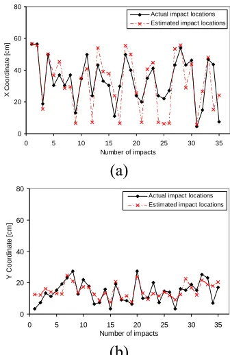
Impact location results are given in Figure 8 and Figure 9. These two figures results compare the actual impact locations and estimated impact locations in terms of

their x and y coordinate, respectively. The

experimental wave velocity characteristic was used for impact location in Figure 8, whereas the FE-modelled wave velocity characteristic was used in Figure 9.

0 20 40 60 80

0 5 10 15 20 25 30 35 Number of impacts

X C oor di nat e [ c m ]

Actual impact locations Estimated impact locations

(a) 0 20 40 60 80

0 5 10 15 20 25 30 35 Number of impacts

Y C o or di na te [c m ]

Actual impact locations Estimated impact locations

(b)

Figure 8: Impact location estimation based on the experimental wave velocity characteristic:

(a) x coordinate (b) y coordinate.

0 20 40 60 80

0 5 10 15 20 25 30 35 Number of impacts

X C oordi nat e [c m]

Actual impact locations Estimated impact locations

(a) 0 20 40 60 80

0 5 10 15 20 25 30 35 Number of impacts

Y C oor di nat e [ c m ]

Actual impact locations Estimated impact locations

(b)

Figure 9: Impact location based on the FE

wave velocity characteristic: (a) x coordinate

These results show that although the overall trends of the actual location curves are followed by the estimated location

curves, there exist discrepancies in x and y

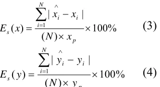
coordinate estimates. The difference between the actual and estimated impact coordinates was calculated as an average distance. The percentage error of average distance per axis can be calculated as

% 100 ) ( | | )

( 1 _×

× − =

∑

E (3)

% 100 ) ( | | )

( 1 _×

× − =

∑

E (4)

where for a given total of N impacts on the

composite structure, x∧ and are the

predicted coordinates, x and y are the actual

coordinates, and x

∧ y

p and yp are the size

structure in the x and y coordinate axes.

The impact location performance was also assessed using a percentage error expressed in terms of the total area of the plate, given by

( )2 100%

1 _× × − × − = ∧ = ∧

∑

x _{i i}

N i i i A structure of area

ε (5)

Table 2 gives a summary of all the analysed errors. These results indicate that the GA-based algorithm has produced good estimates over the impact area. The maximum area error was less than 2% of the total area of the plate. It is also important to note that the FE-modelled wave velocity characteristics have given a relatively good performance if compared with the experimental wave velocity characteristics; their 1.72% error is only slightly larger than the 1.5% experimental error.

Table 2: Summary of analysed errors

Exp FE

Average error (x coordinate) [mm] 70.47 86.06

Average error (y coordinate) [mm] 39.36 36.84

Percentage error (x coordinate) [%] 11.59 14.15

Percentage error (y coordinate) [%] 12.95 12.11

Total error per analysed area [%] 1.50 1.72

5. Conclusion

Impact location of a composite plate was obtained with maximum area error was less than 2% of the total area. A good agreement between the experimental and simulated results was obtained in terms of wave propagation velocity, arrival time and nonlinear behaviour versus propagation direction. Strain data can be used together with the genetic algorithm in estimating the impact location. The simulated strain data from FE modelling can be used to simplify the analysis.

References

[1] Z. Aslan, R. Karakuzu and B. Okutan, Composite Structures, 59, pp. 119-127, 2003 [2] F.Mili and B. Necib, Composite Structures, 51, pp. 237-244, 2001.

[3] S.S. Kessler, S.M. Spearing and C. Soutis, Smart Materials and Structures, 11, pp. 269-278, 2002

[4] W.J. Staszewski, C. Biemans, C. Boller and G.R. Tomlinson, Key Engineering Materials, 221-222, pp. 389-400, 2002.

[5] D. Weems, H.T. Hahn, E. Grandlund and I.G. Kim, Proceedingsof the 47th Annual Forum of the American Helicopter Society,1991. [6] K. Worden and W.J. Staszewski, Strain, 36, pp. 61-70, 2000

[7] P.T. Coverley and W.J. Staszewski, Smart Materials and Structures, 12; pp. 1-9, 2003 [8] Q.Wang and X.Deng, Int. Journal of Solid and Structures, 36; pp.3443-3468, 1999.

[10] R. Seydel and F.K. Chang, Smart Materials and Structures; 10(2), pp. 354-369, 2001

[11] F.K. Chang, Proceedings of the 4th European Conference on Smart Materials and Structures, 2nd Int. Conf. on Micromechanics, Intelligent Materials and Robotics, Harrogate, UK, pp. 771-781, 1998.