An Approach to Parallel Simulation of Ordinary Differential Equations

http://dx.doi.org/10.4236/jsea.2016.95019

How to cite this paper: Carl, J.D. and Biswas,G. (2016) An Approach to Parallel Simulation of Ordinary Differential Equa-tions. Journal of Software Engineering and Applications, 9, 250-290. http://dx.doi.org/10.4236/jsea.2016.95019

An Approach to Parallel Simulation of

Ordinary Differential Equations

Joshua D. Carl1_{, Gautam Biswas}2

1_{Department of Electrical Engineering and Computer Science, Milwaukee School of Engineering,}

Milwaukee, WI, USA

2_{Department of Electrical Engineering and Computer Science, Vanderbilt University, Nashville, TN, USA}

Received 19 March 2016; accepted 28 May 2016; published 31 May 2016

Copyright © 2016 by authors and Scientific Research Publishing Inc.

This work is licensed under the Creative Commons Attribution International License (CC BY). http://creativecommons.org/licenses/by/4.0/

Abstract

Cyber-physical systems (CPS) represent a class of complex engineered systems where functionali-ty and behavior emerge through the interaction between the computational and physical domains. Simulation provides design engineers with quick and accurate feedback on the behaviors gener-ated by their designs. However, as systems become more complex, simulating their behaviors be-comes computation all complex. But, most modern simulation environments still execute on a sin-gle thread, which does not take advantage of the processing power available on modern multi-core CPUs. This paper investigates methods to partition and simulate differential equation-based mod-els of cyber-physical systems using multiple threads on multi-core CPUs that can share data across threads. We describe model partitioning methods using fixed step and variable step numerical in-tegration methods that consider the multi-layer cache structure of these CPUs to avoid simulation performance degradation due to cache conflicts. We study the effectiveness of each parallel simu-lation algorithm by calculating the relative speedup compared to a serial simusimu-lation applied to a series of large electric circuit models. We also develop a series of guidelines for maximizing per-formance when developing parallel simulation software intended for use on multi-core CPUs.

Keywords

Parallel and Multi-Thread Programming, Ordinary Differential Equations, Simulation

1. Introduction

can occur, locally, within a system, or be distributed in a networked environment [1]. CPSs are also frequently designed to include human decision making as part of the control of the physical system.

Systems engineering methods play an important role in designing and analyzing CPSs. In the traditional ap-proach to systems engineering, design has followed a discipline by discipline apap-proach, with individual compo-nents being created in isolation to meet specified design criteria. After the individual, compartmentalized, design phases, all of the components are brought together for integration testing to verify that the design criteria are met [2]. This method works well for simpler systems with few interacting components and physical domains.

With the increasing prevalence and complexity of present-day CPSs, the traditional systems engineering ap-proach is proving to be detrimental to the overall design process. Several research papers, such as [1]-[5], have discussed in detail the problems and challenges involved in designing and building CPSs. For CPSs, to analyze and understand the behaviors of the system requires methods by which the different component models can be composed and analyzed both as a full system and as individual components. One approach is to build all of the components in a virtual design environment, and use simulation to perform integration testing throughout the design process [4]. At the beginning of the design the different components can be represented by low fidelity models, possibly taken from a component library, and composed to form an initial design of the final system. As the design progresses the initial models can be replaced with more specific and detailed models, including the final component implementations. At all points in the design process the composed system can be simulated, providing a means to analyze how the integrated system performs [4]. Simulation, therefore, provides a very tight design-test-redesign feedback loop for the designer. Any changes or tweaks to the model can be made quickly and simply in the virtual design environment and the test re-run to verify for correctness.

[image:2.595.116.524.457.708.2]

Previously, the increasing complexity of systems and the corresponding increases in their computational complexity were matched by faster processor speeds that kept the simulation runtime within reasonable bounds. However, since the year 2005 processor clock speeds have largely leveled off (seeFigure 1), and the increase in computing power for commercial chips has been achieved by adding processor cores that can execute in parallel rather than by increasing clock speed [6]. Exploiting this parallel processing power provided by multi-core ar-chitectures to improve the run time of a simulation requires algorithmic changes to the simulation; one has to develop parallel versions of the simulation algorithms to speed up the computation. However, developing these parallel simulation algorithms will require careful consideration of the physical CPU architecture to derive the best parallel performance.

252

Modern CPUs have several layers of memory between the physical CPU registers and the main system mem-ory collectively called the cache (the cache is discussed in more detail in Section 3.1.2). The cache allows CPU core to keep data that it is currently working on readily available in a layer of cache that provides very quick access, and allows data that is not needed to stay in a layer of cache farther away from the core [7]. The cache also allows the physical computation cores to communicate with each other. Mismanagement or ignoring the structure of the CPU cache in a multi threaded program can have a drastic negative impact on the program ex-ecution performance [7]-[9], and therefore, parallel software design on a multi-core CPU requires careful con-sideration of both how to partition the computational problem into independent pieces suitable for parallel si-mulation, and how those independent pieces interact with each other and the on chip memory.

The potential parallel processing power of modern multi-core CPUs, coupled with the potential performance pitfalls of the CPU cache, leads us to focus our research into parallel simulation algorithms that target a mul-ti-core CPU and use the CPU cache as a performance asset instead of a liability.

The goal of this paper is to take steps toward facilitating the design process for cyber-physical systems by re-ducing the time it takes to simulate complex and large system models by developing parallel simulation algo-rithms for multi-core CPU architectures. A primary component of these algoalgo-rithms is the incorporation of suita-ble memory management and the use of program constructs that take advantage of the CPU memory architec-ture. Our research contributions, therefore, focus on:

1) Developing classes of parallel simulation algorithms that appropriately uses the multiple cores and the cache memory organization on a multi-core CPU, and

2) Running experimental studies that help us analyze the effectiveness of various multi-threading and memory management schemes for parallel simulations.

The contents of this paper are as follows. Section 2 describes our simulation methodology. Section 3 de-scribes our shared memory parallel processing architecture. Section 4 our approach to parallel simulation of or-dinary differential equations and the models that we use to evaluate our algorithms. Section 5 presents our pa-rallel simulation algorithms and experiment results. Section 7 presents our conclusions regarding papa-rallel simu-lation of ordinary differential equations.

2. Simulation Methodology

This section provides definitions and derivations related to simulation (Section 2.1), describes our approach to simulation (Section 2.2), the numerical integration methods we use to perform our simulations (Section 2.3), and an overview of inline integration (Section 2.4).

2.1. Definitions and Discrete Time Derivation

The physical systems we will be working with are continuous dynamic systems, and are modeled using ordinary differential equations (ODE) or differential algebraic equations (DAE). ODE models are represented mathemat-ically in the state equation form

( )

t = x

(

t,

( ) ( )

t , t

)

. 

x f x w (1)

where x

( )

t is a vector of the state variables of the system, with a corresponding derivative vector x

( )

t .

( )

t

w is the set of algebraic variables, which includes the input variables. nx is the number of state variables, and nw is the number of algebraic variables [10]. The vectors x

( )

t and x

( )

t have the same dimensions equal to nx. The functional form fx specifies the values of the derivatives of each state variable, which when integrated provides the evolution of the system behavior, xt over time. The continuous time ODE set,

( ) ( )

(

, ,

)

x t t t

f x w , can be expressed in discrete-time form by plugging Equation (1) into a numerical integration method, the Forward Euler method from Equation (3) in this case [11]:

(

)

1 , ,

n+ = n+ ⋅h n tn n n

x x f x w (2)

represented by h, is small, the first order approximation above is quite accurate.

One important point to note from Equation (1) is that the calculation of any value in x

( )

t does not depend on any other values of x

( )

t because no value of x

( )

t appears as inputs to the function fx. This means that the calculation of the specific values in x

( )

t can happen in any order.

Solving the functions in fx is called a function evaluation.

Definition 1 (Function Evaluation) A function evaluation is one evaluation of the vector function f from Equation (1).

There is one equation for each variable that is not a state variable, that is, one equation for each element in the sets x

( )

t and w

( )

t , which makes the system just determined. At time point, ti, the state variable derivatives,

( )

ti 

x are integrated using a numerical integration method to calculate the values of the state variables at time

( )

ti+1

x . This interaction between x

( )

t and x

( )

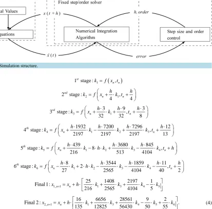
t relate to the structure of a simulation, and is reviewed in Section 2.2. Integration methods are reviewed in Section 2.3.

2.2. Simulation Structure

The goal of a simulation is to generate time trajectory data for all of the variables in the dynamic system model. The high-level process is shown in Figure 2. The simulation is performed in discrete time, so the relevant variables are functions of the simulation step, xn, instead of time, x

( )

t . Each value of n represents a specific point in time, t. The value of t at the next time step, n+1, is t+h, where h is the time step of the simulation, which the amount of time between time steps.

In modern simulation software the model compiler converts the declarative DAE model to explicit ODE form [12]. The ODE set of equations calculate the values of the derivatives of the state variables, xn (Equation (1)). After the state variable derivatives are calculated, the simulation software passes the calculated derivatives to the chosen solver.

Definition 2 (Numerical Integration Method) The numerical integration method integrates the derivative of a

variable at time t to determine the value of the corresponding state variable at time t+h, where h is the simu-lation step size.

Definition 3 (Step Size) The step size of a simulation is the distance between two individual time steps, and, depending on the solver, it may be kept fixed or dynamically adjusted during simulation. It is described by the variable h in definition 2.

Definition 4 (Solver) The solver is a standalone piece of software that implements a specific numerical inte-gration method, and, potentially, step size control, order control, and any other tasks necessary to accurately complete a simulation [13].

The solver uses a numerical integration method to integrate the derivatives to find the new values of the state variables at the next time step, xn+1, or in continuous time representation x

(

t+h

)

. The values are checked to

guarantee that the results are within the prescribed error tolerance. If they are not then the solver takes an appro-priate action, usually halving the simulation step size, and tells the simulation code to re-evaluate the previous time step with the smaller step size. If the state variables are within the defined tolerance, the new state variables are passed to the computational model which then calculates the next values of the state variable derivatives. The solver can also take the step of making the simulation step size larger if a small step size is no longer needed. This process continues until the simulation stop time is reached.

The two aspects of the simulation, shown inFigure 2, the computational model and the solver are generally two separate pieces of software. This allows different integration algorithms to be paired with the same model by simply changing a setting in the overall modeling environment.

2.3. Integration Method Overview

The numerical integration methods that we use in this work are the Forward Euler (FE), and Runge-Kutta- Fehlburg 4-5 (RKF45). The FE method is defined as [11]:

1 .

n n n

[image:5.595.125.539.115.522.2]

254

Figure 2. Simulation structure.

(

)

1

1 stage :st ,

n n

k = f x t

2 1

2 stage : ,

4 4

nd

n n

h h

k = f x_ + ⋅k t + _

 

3 1

3 9 3

3 stage : ,

32 32 8

rd

n n

h h h

k = f x_ + ⋅ ⋅ +k ⋅ t + ⋅ _

 

4 1 2 3

1932 7200 7296 12

4 stage : ,

2197 2197 2197 13

th

n n

h h h h

k = f x_ + ⋅ ⋅ −k ⋅ ⋅ +k ⋅ ⋅k t + ⋅ _

 

5 1 2 3 4

439 3680 845

5 stage : 8 ,

216 513 4104

th

n n

h h h

k = f x_ + ⋅ ⋅ − ⋅ ⋅ +k h k ⋅ ⋅ −k ⋅ ⋅k t +h_

 

6 1 2 3 4

8 3544 1859 11

6 stage : 2 ,

27 2565 4104 40 2

th

n n

h h h h h

k = f x_ − ⋅ ⋅ + ⋅ ⋅ −k h k ⋅ ⋅ −k ⋅ ⋅ −k ⋅ t + _

 

1_ 1 1 3 4 5

25 1408 2197 1

Final 1:

216 2565 4104 5

n n

x + =x + ⋅h  ⋅ +k ⋅ +k ⋅ − ⋅k k 

 

2_ 1 1 3 4 5 6

16 6656 28561 9 2

Final 2 : .

135 12825 56430 50 55

n n

x + =x + ⋅h  ⋅ +k ⋅ +k ⋅ −k ⋅ +k ⋅k 

  (4)

This method is really 2 separate RK methods that share their initial stages. One method is a 4th order method that uses stages 1 through 5 and equation Final 1, and the second method is a 5th order method that uses stages 1 through 6 and uses equation Final 2. This makes determining the error for the simulation trivial. The error for a time step is evaluated according to:

1_n1 2 _n1 .

x + −x + < (5)

If Equation (5) is false then the simulation needs to choose a new step size and recalculate the time step. If Equation (5) is true then the time step is accepted by the solver and the 5th order value of xn+1 is propagated to

the next time step. If the difference calculation in Equation (5) is below both the error threshold and a separate step size threshold, then the solver may choose to make the time step greater.

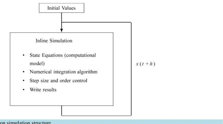
2.4. Inline Integration

[image:6.595.177.539.83.285.2]

Figure 3. Inline integration simulation structure. integration is used. By itself, inline integration will not necessarily yield a reduction in simulation time, but it will provide a means for parallelizing the integration method with the model, and open up other opportunities for reduce the simulation time.

3. Shared Memory Parallel Processing Architecture

Traditionally computing architectures have been described in terms of four qualitative categories according to Flynn’s taxonomy [16] [17]:

1) Single Instruction, Single Data (SISD): This architecture is a conventional sequential computer with a single processing element that has access to a single program data storage.

2) Multiple Instruction, Single Data (MISD): In this architecture there are multiple processing elements that have access to a single global data memory. Each processing element obtains the same data element from mem-ory, and performs its own instruction on the data. This is a very restrictive architecture, and no commercial pa-rallel computer of this type has been built [17].

3)Single Instruction, Multiple Data (SIMD): In this architecture, multiple processing elements execute the same instruction on their own data element. Applications with a high degree of parallelism, such as multimedia and computer graphics, can be efficiently computed using a SIMD architecture [17]. Modern tools for parallel processing large amounts of database information, such as Hadoop [18], are closely related to the SIMD archi-tecture.

4) Multiple Instruction, Multiple Data (MIMD): In this architecture, there are multiple processing elements and each element accesses and performs operations on its own data. The data may be accessed from local mem-ory on the processor, from shared memmem-ory, i.e., memory shared by multiple processor units.

3.1. Multi-Core CPU

Multi-core CPUs, such as Intel’s Core line of processors [19] and AMD’s FX processors [20], are the backbone of modern engineering workstations and are an example of MIMD parallel architecture. We are targeting im-proved performance of simulation on engineering workstations so the MIMD architecture will be our focus in this research.

At a conceptual level, the CPU can be divided into two parts: the computational processor, and the memory. Our primary focus will be on the processor memory, which is covered in Section 3.1.2, but we will first sum-marize the important aspects of the processor as it relates to the memory system.

3.1.1. Processor

256

Definition 5 (Thread) A single program execution stream that includes the program counter, the register state and the stack[21]. Multiple threads can share an address space, meaning threads can access memory used by other threads. Due to this shared address space, a processor can switch between threads without invoking the operating system.

Definition 6 (Hardware Multithreading) Increasing utilization of a processor by switching to another thread when one thread is stalled due to causes such as waiting for data from memory, or a no operation instruction [21].

Definition 7 (Process) A higher level computation unit, above threads. A process includes one or more threads, the address space, and the operating system state. Changing between processes requires invoking the operating system [21].

CPU hardware that implements hardware multithreading is designed such that each hardware thread is pre-sented to the Operating System (OS) as an individual CPU, which gives the OS double the number of cores to use for computational work. In our work, we treat these multithreaded processors as individual processors, just like the OS, so that a computer with 4 cores that supports 8 threads (2 threads per core) is treated as having 8 unique cores.

3.1.2. Cache

The cache memory hierarchy is the memory closest to each processor core. The cache closest to each core is called the L1 cache, and, in a 3 level hierarchy such as Intel's Core architecture [19], the cache farthest away from the core is called L3. Beyond the L3 cache is the main system memory (RAM). An example of the Intel Core i7 cache structure is inFigure 4. In the Intel i7 the L1 cache is split into an instruction cache and a data cache, and each L1 and each L2 cache are usable by only 1 core, while the L3 cache is shared across all cores. This L3 cache allows the individual cores to exchange data, and the L1 cache is used to keep frequently used data readily available, as cache access times become longer the farther away the level of cache is from the core. Also, the cache levels that are farther away from a processor are going to be larger than the levels closer to the processor. On the CPU we use to perform our experiments in Section 5 each L1 cache is 32 KB, each L2 cache is 256 KB, and the L3 cache is 8 MB [19].

In most cases, the cache is implemented as a hierarchy, where data cannot be in the L1 cache without it also being in L2 and L3 [22]. More formally:

if x=some data (6)

1 2 3.

[image:7.595.140.499.509.703.2]

x∈L ⇒ ∈x L ⇒ ∈x L ₍₇₎ In order for processors to communicate or exchange data, the data needs to be in the layer(s) of cache that are shared across cores. Usually, as shown in Figure 4, this is the cache that is the farthest from the processor, and

therefore the slowest layer of cache. As an example, since the threads can only directly access their L1 cache, to send data from Core 0 to Core 2, Core 0 will first have to write its data to the L1 cache. Then Core 2 will request the data through a load or get instruction. The memory controller on the chip will then move the data from the L1 cache on Core 0, to the L2 cache on that core, and then to the global shared L3 cache. After it is in the L3 cache the data will be moved into the Core 2 L2 cache, and finally into the L1 cache on Core 0 where the data can finally be used.

The cache is organized into cache lines, or blocks.

Definition 8 (Cache Line) The minimum unit of information that can be present or not present in a cache

[22].

Definition 9 (Cache Line Read) The process of pulling a cache line from a cache far away from a CPU core to a cache close to the CPU core.

In most modern desktop processors the cache line is 64 bytes. This means that moving 4 bytes of data (typi-cally, the size of an integer in C/C++) to the L1 cache will move the entire 64 byte cache line that contains the requested 4 bytes of data. Multiple threads in different cores accessing data in the same cache line can lead to a problem known as cache line sharing.

Definition 10 (Cache Line Sharing) When two unrelated variables are located in the same cache line are be-ing written to by threads on separate cores, the full line is exchanged between the two cores even though the cores are accessing different variables [22].

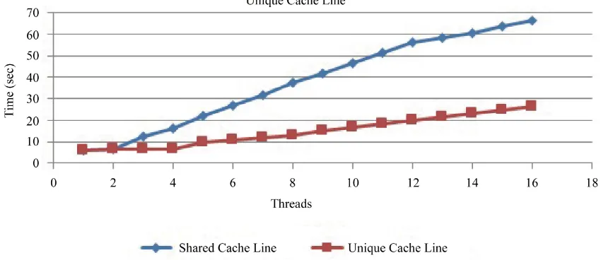
Cache line sharing can have a dramatic impact on performance, which can be demonstrated through a simple experiment (modified from [8]). We create a large array of data, and a varying number of threads, from 1 up to n, where n is equal to 2 times the number of processors recognized by the operating system. We assign each thread a location in the array on which to perform some work. Since arrays are stored in contiguous memory, if we as-sign threads 1 through n indexes in array from 0 through n−1, the threads will all be working with data on the same cache line. If we assign each thread an index in the array of 0 through

(

n−1

)

∗ variables in a cache line then each thread will be working with data on separate cache lines. The expectation is that the execution times when the threads are working on the same cache line will be much longer than the execution times when the threads are working on separate cache lines.

[image:8.595.100.525.510.694.2]

This experiment was performed on a machine running Ubuntu 15.04 with an Intel i7-880 CPU clocked at 3.08 GHz and 8 GB of RAM. This CPU has 4 physical cores that each support 2 hardware threads, the same archi-tecture asFigure 4. The experiment was run 20 times and the computation times averaged. The results of the experiment are shown in Figure 5. The results show that when a cache line is shared across threads, as the number of threads increases the computation time increases as well; nearly linearly in terms of the number of threads. The results also show that when the threads each have their own cache line, there is very little increase

258

in the computation time when using 1 through 4 threads. This is expected as the threads are working on inde-pendent cache lines and do not interfere with each other. The jump in computation time above 4 threads is likely due to hardware limitations of Intel’s hardware multithreading implementation (marketed as Hyperthreading by Intel [19]). There may appear to be 8 unique CPUs to the operating system, but the physical hardware cannot accurately mimic 8 independent cores when there are only 4 physical cores to work with. When using 4 threads, the method using independent cache lines is 2.9 times faster than the implementation using a shared cache line.

As this example shows, sharing cache lines between threads can lead to significant performance problems, and should be avoided [8] [21]. One method to avoid cache line sharing is to use cache aligned data structures.

Definition 11 (Cache Aligned Data) Cache Aligned Data is data that has a memory address that is an even

divisor of the cache line size. That is, in most modern architectures, cache aligned data has memory address modulo 64 = 0.

In effect, a cache aligned data structure was used in the above example where each thread was assigned an array index in which to work that was on its own cache line. Programmers need to consider the processor cache, and avoid cache line sharing, when designing multithreaded applications to ensure program performance.

4. Parallel Simulation of Ordinary Differential Equations

This section presents our general approach to simulating our models (Section 4.1), a mathematical description of model partitioning (Section 4.2), a discussion on the overhead associated with running parallel simulations (Sec-tion 4.3), the models that we used to evaluate our algorithms (Sec(Sec-tions 4.4 and 4.5), our experiment configura-tion (Secconfigura-tion 4.6), and our base test case (Secconfigura-tion 4.7).

4.1. Model Simulation

The state equations can be integrated independently and in any order for each time step (Section 2.1). This gives us freedom, within a time step, to group the state equations in ways that achieve the best run time performance. At the end of a time step, the updated state variable values will need to be synchronized across the state equa-tions of the system, to allow the different execution threads to acquire the updated state variable values before starting the calculations for the next time step.

We implemented two types of integrators for the parallel simulation algorithms: 1) a fixed-step Euler integra-tor, and 2) a variable-step Runge-Kutta integrator. We discuss our implementations for the two integration schemes next.

4.1.1. Fixed Step Integration

We used an Inline Forward Euler (IFE) integration method [11] (Equation (3)) for all of our fixed step simula-tions. Each step of a Forward Euler (FE) integrator in discrete time is described as:

1 ,

n+ = n+ ⋅h n

x x x (8)

where h is the step size. Inlining the integration equation allows our simulation to calculate xn+1, in a single

eq-uation instead of two eqeq-uations one calculating the derivative of the state variable, xn, and then a second calcu-lating the value of the state variable at xn+1, as is traditionally done in simulation (see Section 2.2). In this case,

inline integration works by taking the equation for ODEs, Equation (1), which solves for x

( )

n and substituting that equation into the equation for FE integration, Equation (8), i.e.,

(

)

1 , , .

n+ = n+ ⋅h x tn n n

x x f x w (9)

We simplify the definition of this equation to be:

(

)

(

)

1 , , , ,

n+ = IFE h n x tn n n

x f x f x w (10)

During simulation using the IFE method, for each time step the simulation calculates the values for xn+1

during time step n. After all of the values for xn+1 are calculated the simulation copies xn+1 into xn:

1.

n = n+

,

n n

t = +t h (12) where t is the simulation time and h is the time step. Then the simulation loops and repeats the process until the simulation reaches the simulation end time. In our fixed step simulations the step size of the simulation is passed as a parameter to the simulation at run-time. The simulation algorithm using IFE integration is described in Al-gorithm 1.

4.1.2. Variable Step Integration

We used an explicit Runge-Kutta-Fehlberg 4,5 (RKF4,5) solver (described in Equation (4)) from the GNU Scientific Library (GSL) [23] for our variable step simulations. The GSL implements the RKF4,5 as a standa-lone solver that follows a traditional approach to simulation, as described in Section 2.2 and shown inFigure 2. To use the solver we supply a function for calculating the derivatives of the state variables, Equation (1), and a function for calculating the system Jacobian matrix. The solver determines the time step size, performs the inte-gration, and maintains the synchronization between time steps. The simulation algorithm using the RKF4,5 solver is described inAlgorithm 2. Since this is a variable step solver, we supply an output interval that indi-cates how frequently we want to receive updates to the system state.

4.2. Mathematical Description of Model Partitioning

Partitioning any computational problem into independent components, such that each part can be executed on a separate processor, is the first step to solving the problem in parallel [24]. In our work we rely on simple heuris-tic partitioning schemes, and leave the problem of finding an optimal model partitioning to future work. Even determining simple heuristic schemes has been a non-trivial problem, but our work represents good progress in that direction. The results derived here can influence the algorithms we develop in the future for optimal parti-tioning. Another part to this work, is to investigate the number of parallel threads that produce optimal run-time performance, this means that in our experiments we will vary the number of model partitions we create.

To facilitate the partitioning, it is important to note from Equation (1) is that the calculation of any value in

( )

t



x does not depend on any other values of x

( )

t , because no value of x

( )

t appears as inputs to the func-tion fx. This means that the calculation of the specific values in x

( )

t can happen in any order. This fact allows us to divide the functions represented by fx into subsets, where each subset contains one or more of the equations to compute the derivatives, and is assigned to one of the execution threads on a multi-core CPU. These threads execute in parallel on the CPU, but at the end of each simulation time step the threads will have to synchronize their data to preserve the correctness of the simulation. This approach allows us to parallelize the computation of each time step in the simulation, and should reduce the wall clock-time of the simulation.

Therefore, we take the dynamic system model described in ODE form (Equation (1)), and divide the system into  sets, where  is the number of threads being used. In this work, we partition the equations such that an

Algorithm 1. Algorithm describing simulation using Inline Forward Euler integration.

260

approximately equal number of state variable calculations are assigned to each thread1.

_0 _1 _

n = n + n + + n

    

x x x x (13)

_0 _1 _

n = n + n + + n

x x x x (14)

( ) ( ) ( )

1 1 _0 1 _1 1 _

n+ = n+ + n+ ++ n+ 

x x x x (15)

(

)

(

)

(

)

(

)

0 _0 _

1 _0 _ _0 _

, , , , , ,

, , , , , , , , , .

n n n n n

n n n n n n

t t t t = + +        

f x w f x x w

f x x w f x x w

(16)

Differences in the cardinality of the sets accounts for remainders in integer division of nx . Subsets

(

)

1,, n_xmodulo , will have a cardinality of nx +1, and subsets

(

nx modulo 1 ,+

)

 , will have a car-dinality of nx .

The value of  is dependent on the simulation algorithm. For example, if =nx, there is one state variable per subset in each partition. For all of the other tests  is going to have a value of mtest, where mtest represents the number of threads being used for a test and ranges from 1 to m, where m is the number of parallel threads on the CPU.

As discussed earlier, this partitioning approach allows us to complete the calculations within each time step in parallel, but it will require a synchronization phase at the end of each time step to guarantee correct results. The partitioning, and the memory structure that supports the chosen partition, will differ for each of our parallel mulation algorithms, and the specific differences are highlighted in Section 5, which describes the parallel si-mulation algorithms and the results of the experimental runs with those algorithms.

4.3. Overhead in Running Parallel Simulations

In any parallel program the parallelization adds overhead that is not present in a serial execution of a program. The number of computations per time step of the simulation is the same for sequential and parallel algorithms. However, the overhead generated by parallelization can limit the effectiveness of the parallel implementation. This overhead typically takes the form of scheduling overhead and communication overhead. The created threads need to be assigned, by the operating system, to a CPU core during the thread runtime. It is the responsi-bility of the OS to ensure that all threads are given enough time on a CPU core to complete their work. There is also overhead due to communication between the created threads. This communication overhead does not occur in a single threaded program, but it is necessary in a parallel program synchronization. The run time of a parallel program can be described at a high level as:

wall clock time=computation time+overhead. (17) The challenge in designing parallel software is to minimize the overhead component of Equation (17). This will generally involve two components: 1) the overhead required to manage shared memory between the differ-ent execution threads, and 2) the amount of swapping that needs to be performed when there are more threads than available processor cores. These two components are not independent of each other, and we describe a number of algorithms that trade off these two parameters.

4.4. RLC Simulation Models

We use the Modelica modeling language [25] to create our simulation models. Modelica is a programming lan-guage for describing the behavior of physical systems [25]. At its core, it is an acausal, object oriented, and equ-ation based language for describing physical models using differential, algebraic, and discrete equequ-ations. The language supports hierarchy, model inheritance, and traditional programming language structures such as if-statements, case statements, loops, built-in primitive variable types, and parameters.

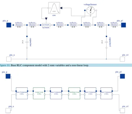
The RLC circuit models were implemented to exploit Modelica’s hierarchical nature, which allows for effi-cient construction of models from individual components. The base component is shown inFigure 6. The in-ductor and capacitor implementations are from the Modelica Standard Library (MSL) [25], version 3.2. The

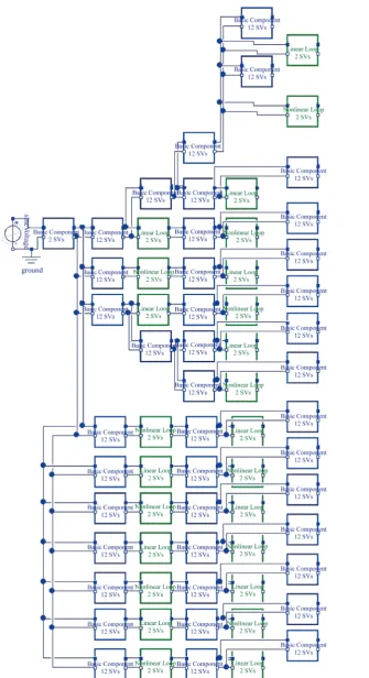
Figure 6. Base RLC component model with 2 state variables. resistor is a modified version of the MSL resistor model. The thermal components were removed from the resis-tor model because they contain Modelica if statements, which can lead to hybrid behavior. The terminals asso-ciated with the components are also from the MSL and were not altered. This set of base components were used to create a larger component with six connected base components as shown inFigure 7. This larger component was used to create the models we used for our experiments. We created a model with 288 state variables that used 24 of the components shown in Figure 8, and we created a model with 804 state variables that used 67 components as shown in Figure 9.

4.5. RLC Models with Algebraic Loops

Algebraic loops are very common in modern complex models [11]. To evaluate the performance of parallelizing the simulation of a model with algebraic loops, we modified the models in Figure 8, andFigure 9 to include components that introduced algebraic loops. We followed the same approach to building the models with alge-braic loops as we did for the models described above: we used Modelica’s hierarchical structure to build com-plex components from the base components. We created 2 new base components, one with a linear algebraic loop and one with a non-linear algebraic loop. They are shown inFigure 10andFigure 11, respectively. The algebraic loop is introduced due to the series resistors ([26] also has an example of series resistors causing alge-braic loops), and, as a result, in these circuit fragments there is no way to uniquely determine the voltage drop across each resistor. Therefore, the voltage drop across the resistors must be calculated simultaneously because the voltage across each resistor depends on the voltage across every other resistor. The non-linear loop is due to one of the resistance values in the loop being a non-linear function of the voltage across another resistor in the loop.

To create models with algebraic loops, we modified the models inFigure 8andFigure 9 by replacing some of the components in Figure 7 with the components inFigure 10 and Figure 11 to create the component in

Figure 12. These new models are shown in Figure 13 and Figure 14. The loop components we added were split approximately evenly between the linear loop components and non-linear loop components.

4.6. Experiment Configuration

We used two sets of parameter values in our experiments. The first set of values set all parameters equal to 1, and the resulting electrical circuits have slow time constants. A parameter value of 1 for all an electrical com-ponents of a circuit is not realistic for most applications, but it was useful for an initial evaluation of a parallel algorithm. We also used more realistic parameter values of 15 Ω for all resistors, 15 mH for all inductors, and 250 µF for all capacitors. The circuits using these parameters had much faster time constants.

We will measure the simulation run time using the wall-clock time of the simulation.

Definition 12 (Wall-Clock Time) The wall-clock time of a simulation is the time it takes from an external us-er’s perspective for the overall simulation to be completed, i.e. the time for a simulation to complete as meas-ured by a clock on a wall.

[image:13.595.109.539.78.715.2]

262

Figure 7. RLC component model with 12 state variables.

[image:14.595.168.525.85.707.2]

[image:15.595.76.539.81.234.2]

264

[image:15.595.91.538.249.634.2]

Figure 10. Base RLC component model with 2 state variables and a linear loop.

Figure 11. Base RLC component model with 2 state variables and a non-linear loop.

[image:16.595.91.540.80.615.2]

Figure 13. Complex RLC model with 288 state variables and 19 algebraic loops (9 linear and 10 non-linear).

rel. speedup serial . parallel t t

= (18)

[image:17.595.161.497.81.698.2]

266

The simulation programming language used for this study is C/C++, compiled and run on Linux. C/C++ sim-plifies the programming task and generates very efficient execution code. Further, C/C++ also has low-level memory management functions that allow cache-aligned data structures to be created. We target Linux as a si-mulation environment because it provides more control over the created threads, and generally faster execution than Windows.

Unless otherwise noted, all experiments were run on an Intel i7-880 desktop PC clocked to 3.08 GHz with 8 GB of memory running Ubuntu 15.04. The generated C++ code was compiled using g++ version 4.9.2 [27]. All experiments were run 20 times on the models presented in Sections 4.4 and 4.5 for parameter values that created slow and fast behavioral time constants. The experiments were run without writing state variable time trajectory data to disk in order to guarantee more consistent simulation times. To calculate the relative speedup for a par-ticular algorithm and thread count, we calculate the average of the wall clock time for the serial simulation. Us-ing this average we then calculate the relative speedup for each algorithm and thread count. The relative spee-dups are averaged for a thread count, and the standard deviation is calculated from the relative speespee-dups.

4.7. Base Test Case

We focus on comparing our parallel simulation algorithms to the fastest and most basic serial simulation algo-rithm we were able to create. Comparing a parallel implementation to a fast serial implementation of the same problem was advocated by [28] as a means to prove that the parallel implementation provides a practical benefit, and is not simply an academic exercise. The type of serial simulation, either fixed step or variable step, is matched to the type of parallel simulation we are using, so fixed step parallel simulations are compared to a fixed step serial simulation, and variable step parallel simulations are compared to a variable step serial simula-tion.

5. Parallel Simulation Algorithms

A parallel simulation algorithm that appropriately uses multiple cores and the CPU cache has conflicting goals, even though using multiple cores effectively and managing the cache both focus on the physical hardware of the CPU. An ideal program architecture from the standpoint of a multi-core CPU will involve a limited number of parallel computation threads, with very little sharing of data between the threads. An ideal program architecture from the standpoint of the CPU cache might be to divide the program into many very small pieces so that the data being worked on by each thread fits entirely into the size of one cache line. These two ideal architectures are often in conflict with each other, one prefers large partitions and the other small partitions, and finding the right balance between the two is the key aspect of our research.

Partitioning the system of equations, such that the cache can be used effectively to minimize the communica-tion between the execucommunica-tion threads was a key factor that drove the design of the simulacommunica-tion algorithms presented in this section. We focus on 1) Minimizing the communication between execution threads, and 2) Utilizing the fastest communication methods for exchanges that have to take place. We leverage the shared-memory archi-tecture in modern multi-core CPUs so that communication between threads can be handled in hardware as a part of the processor’s cache (parallel architectures and processor cache are covered in Section 3.1). However, we design our algorithms so that they share only a minimum amount of data, as sharing data through the cache across threads also causes computation delays, as we demonstrated in Section 3.1.2.

This section presents the set of parallel simulation algorithms we developed in a progression. The different simulation algorithms varied on how many threads were created, and how the variables in the sets xn+1 and

n

x were divided into blocks of memory corresponding to the created threads. We also paid special attention to minimizing memory sharing across threads, in an effort to maximize the performance of the CPU cache, and by extension the simulation speedup. The differences in memory sharing are a primary differentiator between our simulation algorithms, and a primary driver in reworking the thread assignments.

This section describes definitions related to the simulation threads (Section 5.1), a brief description of the ini-tial algorithms we developed that did not produce good results (Section 5.2), and a detailed description of the algorithms that did produce results (Sections 5.3, 5.4 and 5.5).

5.1. Thread Definitions

268

{

T T T0, ,1 2, , ,T Tmain

}

,

= _{ }

T (19)

where T is the set of all threads in the experiment, T0 through T are the threads created for parallel

execu-tion of the particular simulaexecu-tion algorithm, and Tmain is the primary thread that spawns the child threads and controls the advance of the simulation time steps. The value of  typically ranges between 0 and m−1, where m is the number of CPUs available to the operating system (on a processor that implements hardware multithreading that number of CPUs available to the OS is going to be double the number of cores on the pro-cessor, see Section 3.1). As an extreme we also developed an algorithm where  was set to the number of state Equations (nx) of the dynamic system model. We also define:

{

0, ,1 2, ,

}

spawn⊂ = T T T  T

T T (20)

to identify the threads that were created by the main thread, Tmain, for the simulation. Each algorithm creates one or more memory blocks that will be assigned to the threads. We describe the size of the memory blocks as:

[ ],

M X (21) where M represents a block of memory, and X is the size of that memory. We will also use the symbols →, ←, and ↔ to describe if a thread writes to a memory block, reads from a memory block, or reads and writes to a memory block, respectively. Each of the threads in Tspawn only communicates its status to Tmain and does not have to communicate with any other thread.

Another factor that drove the implementation of our algorithms was to enable fast communication and simple synchronization between hardware threads, i.e. Tspawn and Tmain. Synchronization is handled using shared variables. Simple spin locks are used at synchronization points to pause threads [29]. In a spin lock, a thread continually polls a variable waiting for it to change value, which provides for fast communication to handle synchronization between threads because all communication is handled in hardware through the processor's cache. As soon as the assigned variable is updated in the waiting thread’s cache, a thread can continue its com-putation. Alternatives to spin locks are semaphore or mutex locking, but these locking schemes allow the oper-ating system to move the waiting thread off of the core and replace it with a separate waiting thread. Restarting the original thread will require not only monitoring the semaphore or mutex in question, but also requires the OS to move the thread back onto the core. Whereas this may not be significantly impact computational efficiency for some applications, it can significantly deter the execution time of the parallel simulation algorithms, which require synchronization once or twice a time step. Since the simulation runs complete many time steps (up to 50,000 in some experiments) the extra work by the OS to put the thread back into active processing causes sig-nificant negative impact on the simulation. Spin locks, because the thread stays active, do not suffer from this problem.

5.2. Initial Algorithms

Our initial attempts to produce a speedup did not produce good results. This section summarizes our initial algo-rithms, and the lessons learned from them that were applied to our later algorithms.

5.2.1. Algorithm 1: One Thread per State Variable

Our first parallel algorithm creates a separate thread for each individual function in fIFE (i.e., state equation + inline code for performing an integration step). Therefore:

{

0, ,1 , _x

}

.

spawn = T T  Tn

T

Even for moderately sized models, this results in many more threads than cores available on a typical multi- core CPU (at the time of this writing, typically there are 4 to 8 cores available [19] [20]). This algorithm creates one shared memory block across all threads defined by:

[

2 x

]

, M ⋅n

the number of state variables because there are two variables for each state variable: one to store the current time step value of the state variable (xn), and one to store the next time step value (xn+1). Each of the threads has

read/write access to the single shared memory block: . M

↔

T (22) We also tested a second version of this algorithm that set the thread affinity for each of the created threads, such that the threads were evenly distributed between the processor cores. The expectation with setting the thread affinity is that it would offload the work of dynamically scheduling the threads from the OS and fix the schedule, thus reducing the simulation time.

Definition 13 (Thread Affinity) The thread affinity identifies on which processor a thread is allowed to run.

5.2.2. Algorithm 2: Full Shared Memory with Agglomeration

Our second parallel algorithm agglomerated our state variable calculations so that we could create fewer than x

n threads, where nx is the number of state variables in the model.Algorithm 2partitions fIFE into subsets with each subset executing in parallel on a separate thread. Since each thread contains multiple state equations, each thread requires larger amounts of computational work, and this creates a better balance between the com-putational work and overhead required for scheduling and communication. We developed two different agglo-meration strategies that we call (1) simple aggloagglo-meration and (2) smart aggloagglo-meration.

Algorithm Full Shared Memory Simple Agglomeration, uses a simple agglomeration scheme where the equa-tions in fIFE are partitioned according to the order they were specified in the original model. This means that the first n_x

(

m−1

)

equations were assigned to T0, the second set of nx

(

m−1

)

equations were assigned to

1

T, and so on until all of the equations in fIFE were assigned to the threads in Tspawn. There may be variations in the sizes of the subsets as described in Section 4.2.

Algorithm Full Shared Memory Smart Agglomeration, uses a smart agglomeration scheme that groups the ODE equations, such that the equations that have a large number of dependencies (used a large number of state variables to calculate a particular value of xn+1) were grouped together in the same thread in Tspawn. The idea behind smart agglomeration is to limit the amount of data communication between threads, which reduces the overhead, and, therefore, should reduce the simulation time.

5.2.3. Algorithm 3: Partial Partitioned Memory

This parallel simulation algorithm, Partial Partitioned Memory, is identical to the simple agglomeration ap-proach presented above, except that it partitions xn+1 into m−1 independent memory blocks that match the

subsets of fIFE. This avoids a single large shared memory block across all threads, and the created memory blocks can be represented as:

0 , 1 , , 2 ,

1 1 1

x x x

m

n n n

M M M

m m − m

     

 ₋   ₋   ₋ 

       (23) where each memory block Mx is aligned to a cache line, and each block is writable by only one of the threads in Tspawn. There is also a shared memory block

[ ]

main x

M n (24) that contains the values of xn and is readable by all of the threads in Tspawn, but is only writable by thread

main

T . Since thread Tmain has the same role as Algorithm 1andAlgorithm 2, and it is responsible for synchro-nizing xn+1 and xn, it needs to write to Mmain and read from memory blocks M0,,Mm−2.

5.2.4. Analysis of Early Algorithms

in-270 clude:

1) Do not create more threads than there are processors,

2) Managing thread workload so that the computational work assigned to each thread is greater than the overhead associated with creating the thread,

3) Avoid cache line sharing between computational threads,

4) Evenly divide computational work between all threads, and do not reserve one thread for controlling the simulation and all other threads for computation, and

5) Reduce the communication and dependencies between threads.

The algorithms that did produce a speedup are discussed in detail in the following sections.

5.3. Full Partitioned Memory Parallel Fixed-Step ODE Simulation

The fixed-step simulations that gave us the best performance used fully distributed memory. This means that each thread has its own cache aligned block of memory that it writes to which includes both xn+1 and xn. We tested two different versions of the algorithm, Full Partitioned Memory Minimum Sharing and Full Partitioned Memory Simple Agglomeration.

These two algorithms expand the roles of the threads in Tspawn and the thread Tmain. The threads in Tspawn now perform their own synchronization step when given a signal by Tmain. Thread Tmain, instead of remaining idle when computations are being completed by threads in Tspawn, solves some of the functions in fIFE. The program flow describing these two partitioned memory algorithms is described inFigure 15. Compared to the previous algorithms, the back and forth flow between threads is eliminated. Since each of the threads are re-sponsible for their own synchronization according to Equation (11), the synchronization and advancing simulation time steps, on lines 3 and 4 ofAlgorithm 1, are performed in parallel. The threads in Tspawn pause before synchronizing to make sure all threads have completed calculating their values of xn+1. They proceed to

the synchronization phase of the simulation on a signal from Tmain. The threads again wait after synchronization for a signal from Tmain before they begin to calculate their assigned equations from fIFE. This second syn-chronization point guarantees that there are no race conditions between the threads in T during synchroniza-tion. Even though each thread calculates its own simulation time variable, only thread Tmain can issue a stop signal to the threads in Tspawn when the simulation is complete.

5.3.1. Full Partitioned Memory Minimum Sharing

The first full distributed memory approach, Full Partitioned Memory Minimum Sharing, created memory blocks:

(

)

(

)

(

)

(

)

0 1

2

2 , 2 , ,

2 , 2 .

x x

m x shared x

M n m M n m

M − n m M n m

 ⋅   ⋅       ⋅   ⋅       (25)

Each memory block is created on its own cache line to avoid cache line sharing. Also, it is assigned a subset of variables from xn+1 and xn, and then assigned to a thread in Tspawn. The block of memory Mshared is as-signed to Tmain. This is shown inFigure 16. The memory blocks are structured so that each thread in Tspawn only needs the variables in its memory block and the variables in Mshared to solve its subset of fIFE. Therefore, each thread in Tspawn only writes its assigned xn+1 values to its own block of memory, and only reads from

shared

M . Thread Tmain has control of Mshared, and the variables stored in Mshared are the variables that are needed in more than one thread. To calculate its values of xn+1, Tmain has read access to all of the other mem-ory blocks. This memmem-ory structure is called Minimum Sharing, because each of the threads in Tspawn only share memory with thread Tmain.

[image:22.595.92.527.77.694.2]

[image:23.595.83.539.83.375.2]

272

Figure 16. Figure describing Full Partitioned Memory Minimum Sharing memory structure using 1 thread per CPU core. The dashed lines indicate a read-only relationship.

a cache line. If each thread only writes to one memory block, and all memory blocks are aligned to separate cache lines, then there will be no cache line sharing between threads.

5.3.2. Full Partitioned Memory Simple Agglomeration

The second full distributed memory approach, Full Partitioned Memory Simple Agglomeration. It has the same program flow as Full Partitioned Memory Minimum Sharing, shown in Figure 15, where thread Tmain solves a subset of fIFE but still controls when to terminate the simulation, and the threads in Tspawn synchronize their assigned variables.

The memory approach used in Simple Agglomeration is a little different from Minimum Sharing. Each thread in T has its own local memory block to which it reads and writes, and that represents the subset of values in

1

n+

x for which the thread is responsible. There also is a series of shared memory blocks

0, 1, , 1

shared shared sharedm

M M  M ₋ , where each block is a subset of xn. All of the threads in T can read from all of the shared blocks, but only one thread writes to each shared block. The portion of Mshared that each thread writes to is aligned to a cache line boundary, so there are no cache line sharing problems. The memory model of Full Partitioned Memory Simple Agglomeration is:

(

)

(

)

[

]

[

]

[

]

[

]

0 1

1 0 1 1

, , ,

, , , , .

x x

m x shared x shared x sharedm x

M n m M n m

M − n m M n m M n m M − n m

   

    

 (26) The relationship between the threads and the different memory blocks is shown inFigure 17. With this ap-proach, each of the threads in T needs read access to Mshared, but only writes to its own local block and its own portion of Mshared. This memory design relies on the fact that simply because a thread has access to a piece of memory does not mean that it will read from that memory. The threads in T are designed so that they only read the data they need to calculate their values of xn+1 from the shared memory. This design prevents

[image:24.595.109.530.79.444.2]

Figure 17. Figure describing Full Partitioned Memory Simple Agglomeration memory structure using 1 thread per CPU core. The dashed lines indicate a read-only relationship.

5.3.3. Experimental Runs to Evaluate Speedup

The relative speedups compared to the serial case are shown inTable 1andTable 2. These tables do not include the standard deviations because all of the standard deviations are on the order of 10−2.Figure 18 presents the relative speedups across all models.

FromTable 1we can see that the model with 288 state variables did not produce a speedup compared to the serial case. Since the other models did produce a speedup, the lack of speedup on the smaller model is likely due to the model not having enough computational work to overcome the overhead associated with parallelization.

Table 2 shows the relative speedup when simulating the complex RLC model with 804 state variables (Figure 9). For most thread values Minimum Sharing matches the serial simulation, and in a few cases, such as when the model has fast time constants and is simulated using 4 threads, is able to surpass the serial simulation performance and provide a speedup of up to 1.44. Simple Agglomeration provided a small speedup when using the model with fast time constants, but was only able to match the serial simulation when simulating the model with slow time constants.

We note that Minimum Sharing and Simple Agglomeration have very different wall clock times when they are run only using one thread. This is an unexpected result because the memory differences between the two partitioning approaches should not come into play when only using one thread. The likely reason for the differ-ence in single threaded simulation time is differdiffer-ences in implementation. Version 1 uses C-style structs for sharing data, and version 2 uses C-style arrays. Indexing into an array requires pointer arithmetic, which takes extra time, that is not present when using structs.

[image:25.595.147.485.86.394.2]

274

Figure 18. Figure showing the relative speedups across the models for the Full Partitioned Memory algorithms.

Table 1. Relative speedups for Full Partitioned Memory approaches versions 1 and 2 on the complex RLC model with 288 state variables.

Total Threads Slow Time Constants Fast Time Constants

Min. Sharing Simple Agglom. Min. Sharing Simple Agglom.

1 1.01 0.46 1.01 0.43

2 0.50 0.47 0.62 0.50

3 0.52 0.50 0.66 0.55

4 0.52 0.56 0.65 0.61

5 0.45 0.49 0.58 0.53

6 0.45 0.51 0.59 0.56

7 0.43 0.50 0.55 0.56

[image:25.595.89.539.568.720.2]

[image:26.595.86.537.110.303.2]

Table 2. Relative speedup and standard deviations for Full Partitioned Memory approaches versions 1 and 2 on the complex RLC model with 804 state variables.

Total Threads

Slow Time Constants Fast Time Constants

Min. Sharing Simple Agglom. Min. Sharing Simple Agglom.

1 1.03 0.52 1.00 0.59

2 0.80 0.65 0.92 0.78

3 1.02 0.81 1.21 0.97

4 1.17 1.02 1.44 1.26

5 1.02 0.86 1.24 1.05

6 1.12 0.98 1.34 1.19

7 1.11 1.04 1.37 1.27

8 1.10 1.05 1.39 1.29

804 state variables using fast time constants than slow time constants. A possible explanation is due to the equa-tions in fIFE, for the fast parameters, are more complicated than the equations for the slow parameters. This extra complexity, essentially just the presence of parameter values scaling the state variable values, means that the processor has more computational work to solve each equation and therefore the ratio of cache line reads to computational work goes down, and the cache line reads have less of an opportunity to dominate the run time. This analysis seems tenuous, but since these methods use fixed step integration, the change in model behavior has no effect on the integration (because the step size does not change as a result of system dynamics), and the only real difference between the fast and slow parameter values is the presence of the parameter value terms in the integration equations.

In Figure 18, and in the above tables, we also see that the speedup drops between threads 4 and 5. This is due to the hardware multithreading built into the processor. At 5 threads one of the CPU cores needs to run two threads instead of just one, and, because the cache is allocated to a CPU core, not to a thread, the threads must fight for cache resources. It is also possible that the OS moves the extra thread from core to core to try and bal-ance the workload assigned to each core. But this ends up hurting performbal-ance because each time the thread is moved it must populate the cache on the new core, and is, therefore, not able to realize the benefits of using a cache.

We also see in Figure 18 that in some instances there is a performance drop between using one thread and two threads. We are unsure what causes this.

We performed a mean-squared error analysis on our simulation results for both Minimum Sharing and Simple Agglomeration. The MSE calculations compared the time trajectory data of a single threaded fixed step simula-tion and a parallel simulasimula-tion using 8 threads. In all cases where the simulasimula-tion step sizes were small enough to produce a stable simulation, the error was on the order of 10−16 or smaller, so we did not include the mean square error results here.

5.4. Parallel Algorithms Type 5: Full Partitioned Memory, Variable Step Simulation

A variable step simulation is likely to provide better simulation performance than a fixed-step simulation. This algorithm tests a parallel version of a variable step solver, using a full partitioned memory approach, to deter-mine if further speedups can be found.